Abstract—Large scale Landsat image classification is essential to the production of land cover maps. The rise of Convolutional Neural Networks (CNN) provides a new idea for the implementation of Landsat image classification. However, pixels in Landsat images have higher uncertainty compared with high resolution images due to its 30m spatial resolution. Besides, current deep learning methods tend to lose detailed information such as boundaries along with the stacking of convolutional and pooling layers. To solve these problems, we propose a new method called EMM-CNN based on Pyramid Scene Parsing Network (PSPNet). The EMM-CNN uses entropy to decrease the uncertainty of pixels. Then Markov random field model is employed to construct the connections between neighboring pixels and defined a prior distribution to prevent the cross entropy from sacrificing detailed information for the overall accuracy. Finally, transfer learning based on the pretrained ImageNet is introduced to overcome the shortage of training samples and boost the speed of training process. Experimental results demonstrate that the proposed EMM-CNN is able to obtain classification results with fine structure by decreasing the uncertainty and retaining detailed information of the detected image.
Index Terms—Landsat image classification, convolutional neural network, transfer learning, entropy, MRF model
I. INTRODUCTION
Landsat is an important data source for large scale remote sensing image classification. However, objects belonging to the same class represent various features in different locations. For this reason, performance of traditional classification algorithms on Landsat images is unsatisfied. Maximum Likelihood Classifier (MLC) [1], decision tree (J4.8) [2], Random Forest (RF) [3] and Support Vector Machine (SVM) [4] have been performed on large scale Landsat images for classification. However, these methods did not act as well as they did on high resolution images. The highest overall accuracy on global Landsat image classification acquired by SVM is 64.9%, and overall accuracies of RF, J4.8 and MLC are 59.8%, 57.9% and 53.9%,
Manuscript submitted October, 2018. This work was supported by the Strategic Priority Research Program of the Chinese Academy of Sciences under Grant No. XDA19080302, the National Natural Science Foundation of China under Grant No. 41801233, and the 62-class General Financial Grant from the China Postdoctoral Science Foundation under Grant No. 2017M620947. (Corresponding author: Lianru Gao.)
X. Zhao, L. Gao are with the Key Laboratory of Digital Earth Science, Institute of Remote Sensing and Digital Earth, Chinese Academy of Sciences, Beijing 100094, China (e-mail: [email protected]; [email protected]).
Z. Chen is with the Airborne Remote Sensing Center, Institute of Remote Sensing and Digital Earth, Chinese Academy of Sciences, Beijing 100094, China (e-mail: [email protected])
B. Zhang, X. Yang are with the Key Laboratory of Digital Earth Science, Institute of Remote Sensing and Digital Earth, Chinese Academy of Sciences, Beijing 100094, China, and also with the College of Resources and Environment, University of Chinese Academy of Sciences, Beijing 100049, China (e-mail: [email protected]; [email protected]).
W. Liao is with the Department of Telecommunications and Information Processing, IMEC-Ghent University, 9000 Ghent, Belgium (e-mail: [email protected]).
respectively [5]. Traditional algorithms either use artificial features or learn them from a small set of samples. The quantity of model parameters is limited, which highly restrict the models from learning various features existing in large scale remote sensing images. Therefore, the generalization ability of traditional algorithms is weak [6]-[8].
Deep learning is one of the most popular data driven methods [9]-[12], and can learn the relationship between input and output data by a complex network. Therefore, it can fully utilize the characteristics of training data meanwhile has a high tolerance on variety of the spectral and texture features of the same class. With its rise in computer vision, it was widely used in remote sensing image analysis [13]-[15], and also has been tried in Landsat image classification [16], [17]. The usage of deep learning networks on Landsat image classification mainly concentrates in the following two types, the first is scene classification-based Convolutional Neural Networks (CNN) and the other is semantic segmentation-based CNN.
For the first kind of CNN, it is composed of multi-convolutional layers and fully connected layers. It uses a small patch of pixels as input and outputs the label of the centered pixel [18]-[20]. As its output is the label of the whole image, all the pixels are considered belonging to the same class of the centered pixel. Unfortunately, the label of centered pixel cannot stand for the whole patch of pixels, especially when the centered pixel locates near the boundary. Subject to the size of patch, the receptive field cannot be very large which means the network does not have a chance to see the whole object in the detected image. Thus, it is applicable to small images but is difficult to be applied to large scale Landsat image classification. As shown in references [21] and [22], its applications on large scale Landsat images are heavily influenced by noise.
Semantic segmentation-based CNN is an end-to-end network which inputs the original image and outputs its classification result. Its applications in computer vision are relatively mature [23]-[25], but it is rarely used in remote sensing image classification, especially in large scale Landsat image classification. Reference [26] is an attempt to use semantic segmentation-based CNN on Landsat image, where FCN-8 VGG-16 network produced a Landsat classification result with an average accuracy of 88%. However, almost all the images were used as samples to train the network, which means the classification result is overfitting. Besides, the fine details of roads and small water bodies are post-processed by image masks. Unfortunately, boundary information of the other objects cannot be improved by mask.
Pyramid Scene Parsing Network (PSPNet) employs the resnet module to deeper the network and learn more complex features and its pyramid pooling layer is able to adjust objects with different scales. Thus, it is capable of capturing more details, especially for Landsat images which contains objects with different sizes, such as forest and artificial surface. However, its loss function defined by cross entropy tends to sacrifice accuracies of small objects to ensure the overall accuracy. In other words, the loss function may tend to discard the detailed information. To overcome these limitations, we propose a new framework based on PSPNet for large scales Landsat image classification in this letter. By considering the uncertainty of pixels in
An Entropy and MRF Model-Based CNN for Large Scale Landsat Image
Classification
Xuemei Zhao, Lianru Gao,
Senior Member, IEEE
, Zhengchao Chen, Bing Zhang,
Senior Member,
2 IEEE GEOSCIENCE AND REMOTE SENSING LETTERS, VOL. 38, NO. 5, MAY 2017
Landsat image, we define a new loss function which can maintain detailed information and decrease the uncertainty. In particular, the entropy and Kullback-Lerbler (KL) divergence are exploited to define the loss function in our approach. In addition, an enlarged training set covered 37% of the study area is used to fine-tune the parameters pretrained on ImageNet. With a large quantity of model parameters and the new defined loss function, the proposed EMM-CNN is able to learn various features of the same class in large scale Landsat images and maintain detailed information simultaneously.
The rest of this letter is organized as follows. Study area and data sources are introduced in section II. Section III described details of the proposed EMM-CNN for Landsat image classification. Experimental results are discussed in section IV. Conclusions are drawn in section V.
II. STUDY AREA AND DATA SOURCES
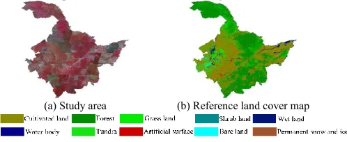
Heilongjiang and Jilin provinces which locate in the northeast of China are chosen as the study area. GLC30 [27] for 2010 is chosen as the reference land cover map. The classification system employed in this letter is the level 1 classes in GLC30 containing 10 classes. Landsat5 images in growing season around 2010 are collected and mosaiced as shown in Fig. 1(a). In this letter, the near infrared, red and green bands are used to train the CNNs. Most of the study area are covered by forest, grass land and cultivated land. Wet land, waterbody, artificial surface and bare land are randomly distributed among them. Sizes of objects are significantly different in the study area, so as the spectral and texture features of the same class (due to their positions and imaging conditions). The study area and corresponding reference land cover map from GLC30 are shown in Fig. 1.
[image:2.612.53.302.374.476.2](a) Study area (b) Reference land cover map
Fig. 1 Study area (a) and corresponding land cover map (b).
III. METHODS
A. Data Preprocessing
Firstly, 585 scenes of Landsat-5 level 1T images in growing season around the year 2010 are collected. Then, the images are stretched and mosaiced (as shown in Fig.1(a)). As the imaging conditions of the collected images are different and there is no accurate radiation correction carried out in this letter, images located in different positions have various radiance values. Thus, the stitching lines are obvious in Fig. 1(a). The GLC30 with 80% overall accuracy is produced by different institutes. Therefore, accuracies in different areas are different. Besides, some parts of grassy river bed are classified to wet land and the others are classified to grass land. To ensure CNNs can learn essential features from the samples, typical samples are manually selected from GLC30. The size of input images
is set to 640640 pixels. So, the study area was divided into 2628
lattices with the same size. Forest land and grass land in the land cover map are heavily influenced by noise. So, only 970 lattices in the study area are selected as samples which possess 37% of the study area. To supplement the samples of forest land and grass land, additional 1554 lattices are added to the sample sets. Then 1/5 of the samples are randomly selected as the validation set, and the other 4/5 samples act
as the training set. In the training set, cultivated land, forest, grass land, shrub land, wet land, waterbody, tundra, artificial surface, bare land, and permanent snow and ice account for 23.23%, 24.40%, 33.56%, 0.50%, 1.29%, 1.24%, 0.00% (780 pixels), 1.35%, 14.21%, and 0.22% of the total area of training set respectively.
Images of the study area should also be clipped to 640640 pixels
for convenience of inference. However, due to the padding process in convolutional layer, boundary information of images is lost along with the stack of CNN layers. To overcome this drawback, images covered
the study area are clipped to 640640 pixels with an overlap of 320
pixels. After the inference process, half of the overlapped pixels are assigned to its nearest classification result from the clipped image. In
other words, each clipped image contributes its middle 320320 pixels
to the final mosaiced classification result, except for the clipped images located in the edges of the whole image.
B. Architecture of the proposed EMM-CNN
The proposed method is an end-to-end network which inputs the whole image and outputs its classification result. The network constructs a non-linear relationship between the input image and the output classification result by learning the semantic features through stacked convolutional layers. The training process is shown as Fig. 3. Firstly, a pretrained resnet module is employed to extract higher level features of the input image. Then, a pyramid pooling layer with four branches is used to fit objects with different scales. After that, a classification layer is carried out to classify the extracted features into the given number of classes. Finally, differences between the classification result and the reference land cover map are measured by an entropy and Markov Random Field (MRF) model-based loss function, and the parameters of the network are updated through backpropagation. The proposed method can be considered as an entropy and MRF model-based CNN, and is called EMM-CNN in this letter.
Fig. 2. Training process of the proposed EMM-CNN.
C. Definition of Loss Function
Loss function is the guidance to optimize the parameters of the network. Therefore, the definition of loss function is the key to obtain accurate classification result. In this paper, we proposed a new loss function composed of cross entropy, entropy and MRF-based KL
divergence. Let P = {pij | i = 1, 2, …, n; j = 1, 2, …, c} be the set of
output feature map obtained from the proposed EMM-CNN and L = {li
| li{1, 2, …, c}; i = 1, 2, …, n } be the corresponding set of labels,
[image:2.612.314.566.401.548.2]cross-entropy
+
entropy KLJ
J
J
J
(1)1) Cross entropy
Cross entropy is a global standard to evaluate the inferenced classification result, and acts as the loss function in most of deep learning networks. It is defined as:
cross-entropy 1
1
n i i iJ
n
l
p
(2)where li is a vector form of scalar li, in which only the lith position is 1
and other positions are 0 with a length c, and pi = {pij | j = 1, 2, …, c}.
To maintain the overall accuracy, detailed information will be sacrificed if the loss function is defined only by cross entropy.
2) Entropy
Since spectral and texture information of Landsat image is unclear, pixels, especially the ones located in boundary have a strong uncertainty. Information entropy is a quantitative description of information. It will be large if an event has a strong uncertainty, or small if the event is almost certain. Therefore, entropy is employed in the loss function to decrease the uncertainty of pixels and increase the accuracy of pixels located in boundary. The output feature map of the PSPNet is considered as the probability of the ith pixel belonging to the jth class. Then the entropy is defined as
entropy 1 11
log
n c ij ij i jJ
p
p
n
(3)For each j, if all pij tends to be 0 and 1, it means the ith pixel has a
certain belongness; otherwise, if pij cluster around their mean value, it
means the ith pixel has a strong uncertainty. The uncertainty of pixels may result in unstable classification result even when a small change appears on the parameters of the network.
3) MRF based KL divergence
In Landsat images, objects with small sizes such as artificial surface, will have much lower accuracy than bigger sized objects as forest. To balance global and local information, MRF is introduced to establish the connections in neighborhood systems. Assume the label of a pixel is determined by the pixel itself and its neighboring ones, then the prior probability of a pixel is defined as
' ' ' ' ' ' ' 1 ' [image:3.612.315.567.392.662.2],
| , , '
=
',
i i i i iij i i i c
i i
j i
exp
V
j l
r
p l
j l
i
exp
V
j l
N NN
(4)where Ni is the neighborhood system of pixel i, i' is the index of Ni, is
a parameter controlling the effect of neighborhood system and Vi' is
,
0,1,
i
i i
i
l j
V j l
l j
(5)
The MRF-based prior probability rij defined above is an indicator of
the similarity between the centered pixel and its neighboring ones. When a pixel locates in the center of an object, the prior probability is larger since more neighboring pixels belongs to the same class with the center one; when a pixel locates near the boundary between two objects, the prior probability is smaller since less neighboring pixels have the same label with it. Due to the similar characteristic with the output features, it can be used as an auxiliary information to cross entropy. Therefore, KL divergence is employed to evaluate the difference between the feature map and the prior probability, and is defined as 1 1
1
log
n c ij KL iji j ij
p
J
p
n
r
(6)D. Optimization
The loss function proposed in this paper is optimized by the Stochastic Gradient Descent (SGD) method to acquire the optimum parameters of the network. Assume parameters of the network is
expressed by = {t | t = {wt, bt}} where wt and bt are the weight and
bias parameters of the tth layer, t is the index of layers. Then the
gradients of the loss function J with respect to the parameters tis
1 1 1
1 1 1 1
log
log
n n c
ij i
i ij
i i j
t t t
n c n c
ij ij
ij
i j t ij i j
p
J
p
Nc
p
p
r
r
p
l
θ
θ
θ
θ
(7)
Then the updating of parameters can be calculated as
1 itr itr t t t
J
lr
θ
(8)where itr is the index of iteration, and lr is the learning rate of the
network.
IV. EXPERIMENTS
A. Experimental Results and Comparisons
End-to-end networks FCN, PSPNet and the proposed EMM-CNN are recoded under Pytorch framework. The network is trained on Titan
XP 4 and optimized by Adam optimizer with an initial learning rate
of 10-4 and a weight decay of 10-4. The momentum and batch size are
set to 0.1 and 12. Fig. 3 shows the classification results of FCN, PSPNet and EMM-CNN. FCN tends to detect more grass land while PSPNet and EMM-CNN are more similar to the reference land cover map.
(a) FCN (b) PSPNet (c) EMM-CNN
Fig. 3. Classification results of FCN, PSPNet and the proposed EMM-CNN.
Fig. 4. Details of classification results, where (a1)-(c1) are the reference land cover map; (a2)-(c2) are classification results of FCN; (a3)-(c3) are classification results of PSPNet; (a4)-(c4) are classification results of EMM-CNN.
2 IEEE GEOSCIENCE AND REMOTE SENSING LETTERS, VOL. 38, NO. 5, MAY 2017
clear boundary exists even though the left part and the right part has no obvious difference in the original Landsat image as shown in Fig. 4(a1). However, CNN-based algorithms do not suffer from this problem. FCN is heavily affected by the inconsistency exists in the training samples and classifies forest as grass land in the middle part (Fig.4(a2)). PSPNet obtains better classification result than FCN. Loss function in the proposed EMM-CNN uses entropy and MRF model to preserve detailed information, and its classification result is better compared with the reference land cover map, FCN and PSPNet. Cloud is a significant problem in large scale Landsat image classification. However, small clouds have less influence to PSPNet and EMM-CNN compared with FCN as shown in Fig. 4(b1)-(b4). Due to different imaging conditions and image acquisition time, stitching lines sometimes are obvious in the original Landsat image. Forest in early grown season has similar spectral features as the grass land and it only possesses a small portion in the training set. Loss function in the proposed EMM-CNN can balance the global and local information and forces the network to learn disadvantage features. Therefore, EMM-CNN obtains better classification result on forest in early grown season compared with FCN and PSPNet, as shown in Fig. 4(c2)-(c4).
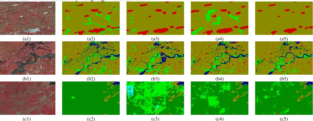
To further evaluate the performance of the proposed EMM-CNN, more detailed images are shown in Fig. 5. Fig. 5(a1) is mainly covered by cultivated land with different growth stages. The darker red is cultivated land double checked by using high resolution remote
sensing images. The reference land cover map classifies the darker red part as grass land. FCN and EMM-CNN correctly recognize it. However, classification results of PSPNet can not classify this part correctly. The dark objects in the upper part of Fig. 5(b1) are paddy field, but they possess small areas. FCN cannot capture the detailed information and classifies the wet land as cultivated land. PSPNet classifies some tiny wet land as forest. Due to the ability of decrease uncertainty and maintain detailed information, EMM-CNN captures more detailed information as shown in Fig. 5(b5). Fig. 5(c1) is mainly covered by forest, but features in this area are complex. FCN is not able to classify this area correctly, and the blurred square areas in Fig.
5(c3) are comprised by lattices with 320320 pixels. It is caused by the
misclassification of each lattice. Similar situation also occurs in PSPNet (Fig. 5(c4)), but the square areas are smaller. EMM-CNN takes the uncertainty of pixels into account and is able to learn more essential features of Landsat images. Therefore, classification result shown in Fig. 5(c5) is much better than those obtained by FCN and PSPNet. Generally speaking, the proposed loss function adopted in EMM-CNN is efficient in decreasing the uncertainty of pixels and retaining detailed information. So, its classification result is able to maintain fine structure even from inconsistency training set with unclear spectral and texture information of Landsat images.
(a1) (a2) (a3) (a4) (a5)
(b1) (b2) (b3) (b4) (b5)
[image:4.612.55.561.312.508.2](c1) (c2) (c3) (c4) (c5)
Fig. 5. Local enlarged images, where (a1)-(c1) are Landsat images; (a2)-(c2) are corresponding reference land cover map; (a3)-(c3) are classification results of FCN; (a4)-(c4) are classification results of PSPNet; (a5)-(c5) are classification results of the proposed EMM-CNN.
B. Accuracies Compared with the Reference Land Cover Map The overall accuracy of the reference land cover map is about 80%, and some parts of the reference land cover map are heavily affected by noise. Besides, grassy river beds are classified to both wet land and grass land in the reference land cover map. Therefore, three areas in reference land cover map visually having high accuracy are selected as ground truth to compare classification accuracies of FCN, PSPNet and the proposed EMM-CNN. The results are reported in Table 1. The selected areas do not contain tundra, bare land and permanent snow and ice. IoU describes the intersection over union of the detected objects and the ground truth. F1 score is the harmonic mean of precision and recall, and the accuracy evaluates the proportion of correctly classified pixels. From Table 1, it can be found that PSPNet and EMM-CNN have higher accuracies than FCN in most of classes, while accuracies of PSPNet and EMM-CNN are similar. Accuracies of grass land are lower due to its similar features with the cultivated land and forest. As shown in Fig. 4 and Fig. 5, the biggest source of error
comes from the mis-classification of the grass land. Usually, forest is adjacent to the grass land, and the mis-classification between forest and grass land are the most in the training set. In addition, the confusion between grass land and wet land in the training set is another factor influencing the accuracy of these two classes. There are not enough features for network to learn to separate grass land and wet land when wet land account for only 1.29% of the total area in the training set. The inconsistency in training set is a significant problem preventing CNN-based methods from learning efficient features of the detected image. The proposed EMM-CNN uses entropy and MRF model to improve its learning ability by decreasing the uncertainty of pixels and balancing global and local information. So, it can learn essential features from imperfect training set and obtains higher accuracy on forest than FCN and PSPNet. The overall accuracy of EMM-CNN is 91.06%, which is higher than 79.09% and 90.07% obtained by FCN and PSPNet.
institute and the classification results between different institutions have significant difference. The chosen three visually high accuracy areas are only served as a reference for quantitative evaluation of the mentioned three methods. Deep learning-based methods learn the features from the training
[image:5.612.43.572.119.216.2]samples, but they are able to obtain consistent classification results even from inconsistent training samples. Due to this powerful learning ability, some areas of the classification results from the proposed EMM-CNN even have better classification results than the reference land cover map.
Table 1. Evaluation results of FCN, PSPNet and EMM-CNN.
(%) IoU F1 score Accuracy
FCN PSPNet EMM-CNN FCN PSPNet EMM-CNN FCN PSPNet EMM-CNN
Cultivated land 78.81 83.25 83.20 88.15 90.86 90.83 86.82 91.17 91.86
Forest 74.51 89.60 91.05 85.40 94.51 95.32 76.78 92.60 94.93
Grass land 9.02 19.32 17.50 16.54 32.38 29.79 49.61 43.30 30.48
Wet land 16.89 22.91 24.27 28.90 37.28 39.06 21.55 25.82 27.04
Water body 57.23 61.71 61.93 72.80 76.32 76.49 81.91 78.76 77.73
Artificial surface 54.57 58.98 54.05 70.61 74.20 70.17 71.82 76.62 63.93
V. CONCLUSION
To overcome the problems in PSPNet of sacrificing detailed information for higher overall accuracy, this letter proposed a new framework for PSPNet by defining a new loss function (using the entropy and MRF model), which is able to maintain fine structure information for large scale Landsat image classification. Partial image of the study area and its neighboring areas are used to construct the training set to avoid overfitting and fine-tuned the parameters pretrained on the ImageNet. Experimental results demonstrate that the proposed EMM-CNN is able to decrease the uncertainty and retain the detailed information, and can obtain classification results with fine details compared with FCN and PSPNet. In our future work, we will focus on enlarging the study area and acquiring enough accurate training samples to achieve more accurate classification results.
ACKNOWLEDGMENT
The authors would like to express their appreciation to GLC30 information service for providing the reference land cover map.
REFERENCES
[1] L. Bruzzone, and D. F. Prieto, “Unsupervised retraining of a maximum likelihood classifier for the analysis of multitemporal remote sensing
images,” IEEE Trans. Geosci. Remote Sens., vol. 39, no. 2, pp. 456-460,
2001.
[2] Y. Zhao, and Y. Zhang, “Comparison of decision tree methods for finding
active objects,” Adv. Space Res., vol. 41, no. 12, pp. 1955-1959, 2008.
[3] M. Belgiu, and L. Dragut, “Random forest in remote sensing: a review of
applications and future directions,” ISPRS J. Photogramm. Remote Sens.,
vol. 114, pp. 24-31, 2016.
[4] F. Zhao, C. Huang, and Z. Zhu, “Use of vegetation change tracker and support vector machine to map disturbance types in Greater Yellowstone
ecosystems in a 1984-2010 Landsat time series,” IEEE Geosci. Remote
Sens. Lett., vol. 12, no. 8, pp. 1650-1654, 2015.
[5] P. Gong, et al., “Finer resolution observation and monitoring of global land
cover: first mapping results with Landsat TM and ETM+ data,” Int. J.
Remote Sens., vol. 34, no. 7, pp. 2607-2654, 2013.
[6] Z. Jiang, S. Shekhar, Overview of Earth Imagery Classification, Spatial Big
Data Science, Springer, 2017.
[7] Q. Wang et al., “Detecting Coherent Groups in Crowd Scenes by Multiview
Clustering,” IEEE Trans. Pattern Anal. Machine Intell.,
DOI:10.1109/TPAMI.2018.2875002, 2018.
[8] Q. Wang, X. He, and X. Li, “Locality and Structure Regularized Low Rank
Representation for Hyperspectral Image Classification,” IEEE Trans.
Geosci. Remote Sens., DOI:10.1109/TGRS.2018.2862899, 2018
[9] Y. LeCun, Y. Bengio, and G. Hinton, “Deep Learning,” Nature, vol. 521,
no. 7553, pp. 436, 2015.
[10] Q. Wang et al., “Scene Classification with Recurrent Attention of VHR
Remote Sensing Images,” IEEE Trans. Geosci. Remote Sens., DOI:
10.1109/TGRS.2018.2864987, 2018.
[11] B. Du, et al., “Stacked convolutional denoising auto-encoders for feature
representation,” IEEE Trans. Cybern., vol. 47, no. 4, pp.1017-1027, 2017.
[12] B. Du, et al., “Exploring representativeness and informativeness for active
learning”, IEEE Trans. Cybern., vol. 47, no. 1, pp. 14-26, 2017.
[13] A. Romero, C. Gatta, and G. Camps-Valls, “Unsupervised deep feature
extraction for remote sensing image classification,” IEEE Trans. Geosci.
Remote Sens., vol. 54, no. 3, pp. 1349-1362, 2016.
[14] E. Maggiori, et al., “Convolutional neural networks for large-scale
remote-sensing image classification,” IEEE Trans. Geoscie. Remote Sens.,
vol. 55, no. 2, pp. 645-657, 2017.
[15] K. Nogueira, O. A. B. Penatti, and J. A. dos Santos, “Towards better exploiting convolutional neural networks for remote sensing scene
classification,” Pattern Recogn., vol. 61, pp. 539-556, 2017.
[16] J. Rebetes, et al., “Augmenting a convolutional neural network with local
histograms – a case study in crop classification from high-resolution UAV
imagery,” Euoropean Symp. Artif. Neural Networks, Comput. Intell.
Machine Learning, 2016, pp. 515-520.
[17] I. H. Ikasari et al., “Multiple regularizations deep learning for paddy
growth stages classification from Landsat-8”, 2016 IEEE ICACSIS, 2016,
pp. 512-517.
[18] W. Li, et al., “Stacked autoencoder-based deep learning for
remote-sensing image classification: a case study of African land cover
mapping,” Int. J. Remote Sens., vol. 37, no. 23, pp. 5632-5646, 2016.
[19] L. Yu, et al., “Convolutional neural networks for water body extraction
from Landsat imagery,” Int. J. Comp. Intell. Appl., vol. 16, no. 1, pp.
1750001, 2017.
[20] A. Sharma, et al., “A patch-based convolutional neural network for remote
sensing image classification,” Neural Networks, vol. 95, pp. 19-28, 2017.
[21] N. Kussul, et al. “Deep learning classification of land cover and crop types
using remote sensing data,” IEEE Geosci. Remote Sens. Lett., vol. 14, no.
5, pp. 778-782, 2017.
[22] A. Sharma, X. Liu, and X. Yang, “Land cover classification from multi-temporal, multi-spectral remotely sensed imagery using patch-based
recurrent neural networks,” Neural Networks, vol. 105, pp. 346-355, 2018.
[23] E. Shelhamer, J. Long, and T. Darrell, “Fully convolutional networks for
semantic segmentation,” IEEE Trans. Pattern Anal. Mach. Inttell., vol. 39,
no. 4, pp. 640-651, 2017.
[24] H. Zhao, et al., “Pyramid Scene Parsing Network,” IEEE Conf. Comp.
Vision Pattern Recog., 2017, pp. 2881-2890.
[25] L. Chen, et al., “DeepLab: Semantic image segmentation with deep
convolutional nets, atrous convolution, and fully connected crfs,” IEEE
Trans. Pattern Anal. Mach. Inttell., vol. 40, no. 4, pp. 834-848, 2018. [26] C. D. Storie, and C. J. Henry, “Deep learning neural networks for land use
land cover mapping,” in Proc. IEEE Int. Geosci. Remote Sens. Symp.
(IGARSS), Valencia, Spain, pp. 3453-3456, 2018.
[27] J. Chen et al., “Global land cover mapping at 30m resolution: a POK-based
operational approach,” ISPRS J. Photogramm. Remote Sens., vol. 103, pp.