International Journal of Innovative Technology and Exploring Engineering (IJITEE) ISSN: 2278-3075, Volume-8, Issue-11S, September 2019
Abstract: Images are the fastest growing content, they contribute significantly to the amount of data generated on the internet every day. Image classification is a challenging problem that social media companies work on vigorously to enhance the user’s experience with the interface. The recent advances in the field of machine learning and computer vision enables personalized suggestions and automatic tagging of images. Convolutional neural network is a hot research topic these days in the field of machine learning. With the help of immensely dense labelled data available on the internet the networks can be trained to recognize the differentiating features among images under the same label. New neural network algorithms are developed frequently that outperform the state-of-art machine learning algorithms. Recent algorithms have managed to produce error rates as low as 3.1%. In this paper the architecture of important CNN algorithms that have gained attention are discussed, analyzed and compared and the concept of transfer learning is used to classify different breeds of dogs..
Keywords : Image classification, Deep Learning, Machine
Learning, Convolutional Neural Network .
I. INTRODUCTION
Convolutional Networks was introduced in the early 1990’s by LeCun et al. [1], they excelled in recognizing digits and faces since their introduction. However the reason why the networks performed exceptionally well was not clear until 2013, when Matthew D. Zeiler and Rob Fergus from New York University gave an insight into the internal working of these machines in [2]. In 2009, Fei Fei Li, a researcher collaborated with Stanford AI and Vision labs and developed ImageNet database [3] that contained 14 million images with more than 20,000 categories. The introduction of this database enhanced the classification algorithms’ performances. It evolved into an annual competition called ImageNet Large-Scale Visual Recognition Challenge (ILSVR) that recognized algorithms that classified objects with the least error rate.
Over the past years many algorithms competed in the annual ImageNet competition, among these was AlexNet [4], a deep learning model which achieved top 5 error rates of 15.3% in 2012. A deep learning model is differentiated from a normal neural network on the basis of depth. The input has
Revised Manuscript Received on September 22, 2019.
Dr. Annapurani. K, Computer Science & Engineering,SRM Institute of Science and Technology [email protected],
Divya Ravilla,Computer Science & Engineering,SRM Institute of Science
and Technology,[email protected]
to surpass several layers in a deep learning model, hence the name ‘deep’ neural
network. In the next few years error rate reduced to a few percent which has been a great development in the vision field. In 2013
ZFNet [2] developed by Matthew D Zeiler and Rob Fergus won the contest with 11.2% error rate and outperformed AlexNet. VGG Net
[5] was the second best model in 2014, the model was based on the authors’ proposal that stated that a model can be improved by increasing the depth of the layers. In 2014, Google developed a deep learning model called GoogLeNet [6] which was also called Inception v1 model, it set a new state- of-art among all the classification algorithms that existed. It set a record by reducing the error rate to 6.7%. ResNet [7], a residual network developed by Microsoft won the ILSVR 2015 competition. Intermediate connections were established in between layers in this network. The authors proved that residual networks are easier to optimize and can provide greater accuracy when the depth of the network is increased. The error rate for ResNet was 3.57% and it surpassed human performance. Based on ResNet architecture two other networks were developed namely Wide ResNets [8] and ResNeXT [9] in 2016. Wide ResNets has smaller depth and larger width while ResNeXT included a new dimension called the cardinality alongside width and height. Also in 2016, a dense convolutional network called DenseNets was introduced in [10] which provided better results with low memory requirement and computation. A relatively new network called the Squeeze-and-Excitation network or SENets [11] won the ILSCRV 2017 with an error rate of 2.251%. The error rate has been significantly reducing since the introduction of deep learning for image classification.
In this paper, we will describe the basic architecture of a deep neural network and the terms that are essential to train a model and use it for classification. The second section will cover the learning procedure. The third section will give a brief overview of the architecture and working mechanism of important models that have participated in the ILSCRV competition and gained popularity in the previous years.
CNN based Image Classification
Model
II. NEURALNETWORKARCHITECTURE
An artificial neural network (ANN) is a computing model developed based on how a biological neural network works to recognize patterns. The biological neural network consists of nerve cells called the neurons that have the ability to transfer or manipulate signals received from the sensory cells, the processing of signal is done in the nucleus of the nerve cell. Millions of these cells together make the biological neural network. The artificial model is made of artificially developed neurons which are embedded with machine learning algorithms and perform the same tasks such as transferring and manipulating the data sent into the system. The artificial neural networks however work only with numerical values which all the existing real-world data can be transformed into. Figure 1.a shows the structure of a brain neuron and Figure 1.b shows the structure of an artificial neuron.Data.
[image:2.595.350.514.146.259.2]Figure 1.a: A nerve cell
Figure 1.b: An artificial neuron
The artificial neuron is called a node, the node is where the computation occurs. The variables X1 and X2 are inputs from either preceding nodes or from the user, W1 and W2 are weights that determine how much each input contributes to the output, the sum of input-weight products is sent to F(X) which is the activation function that links the inputs to the output of the neuron which is Y, the expression can be written as in equation (1).
F(X) determines if the signal from that particular node has to betransferred further or not. If the signal is transferred the node is said to be activated. Activation functions generate values between 0 and 1 or -1 and 1 depending on the function used. There are several activation, the most common ones are ReLU or Rectified Linear Unit, SoftPlus, SoftMax, Sigmoid and Tanh. A layer is made of several nodes, several of these layers make the network. The output of one layer acts as the input to the successive layer. An artificial neural network is
[image:2.595.72.266.293.529.2]represented in Figure 2. Each layer performs a particular task and the network as a whole performs pattern recognition. Each layer recognizes different features, the complexity of the features detected by each layer increases as we move from the input layer to the output layer, since input to a node is the resultant produced with different contributions of previous layers’ nodes.
Figure 2: Artificial neural network
For example, if a network is aiming to classify human faces, the first few layers will detect blobs, edges, curves, corners or other simple features. The next few layers will detect more specific features like the nose or eyes of a human face. The last few layers will combine all the features extracted in the previous layers like the human face parts and detect objects that are made up of these features. This procedure is depicted in Figure 3. This procedure is called feature hierarchy, due to this, the network can work with highly complex data that contains millions of parameters and process them. It does automatic feature extraction unlike many machine learning algorithms that require help from humans.
[image:2.595.305.555.445.532.2]Convolution layer 1 Convolution layer 2 Convolution layer 3 Figure 3: Feature Hierarchy
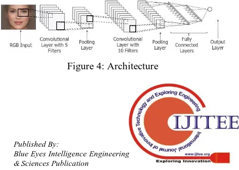
The feature detecting layers are called Convolutional layers since they use convolution to apply filters to images. The network contains pooling layers that help reduce the dimensions of an output produced by a convolutional layer to make the task easier for the succeeding layers. These layers are followed by fully connected layers that combine features to obtain the object. The last layer also called the classification layer like a SoftMax layer calculates the possibility of the image to represent a particular object. This
[image:2.595.315.551.668.836.2]International Journal of Innovative Technology and Exploring Engineering (IJITEE) ISSN: 2278-3075, Volume-8, Issue-11S, September 2019
Architecture is shown in Figure 4. There are many models, some models contain more layers and have different patterns for positioning these layers which makes each model unique.
III. WHYCONVOLUTIONALLAYERS
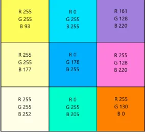
Images are complex than a simple matrix they have many channels. These channels increase the complexity by adding more parameters. We can not create a single vector of all the values in all the channels in the image. An image can be represented in different forms one of which is the RGB. In this the image has three channels namely Red, Green and Blue. This is formed on the scientific basis that says all colors can be represented using these three colors. For example to form say red, the values in channel G and B will be 0 while the value in channel Red will be set to 1. All the values are within the range of 0 and 1. So the sum of all the values in all the channels for a particular pixel will add up to 1. There are other forms to represent color division another one is the 255 band representation. In this the values vary from 0 to 255. Different distribution of the three colors in the RGB format is shown in Figure 5. Every single color can be represented in this form for white all the channels have 255 value and for black all the channels have 0 value. This can be seen in the first column of Figure 5 when the B values is getting closer to 255 the yellow shade is fading and turning into white. Due to these three channels processing of images is more complex than processing a simple vector. By transforming them into a single linear vector we loose the spatial and temporal dependencies among the pixels. Individual colors can be obtained by making the other two channels 0 and by making the desired red, green or blue 255.
[image:3.595.310.536.68.159.2]
Figure 5: RGB Distribution
Convolution applies filters that extract useful information from the images. Filters extract useful information such as lines, curves, corners or blobs. When more layers are present the layers that are stacked above other layers detect more complex features. The convolution process for involves running a matrix called Kernel over the original image. Convolution works on the basis of dot product. The kernel is run over parts of the image and the resultant dot product represents a set of pixels as one. Figure 6 shows the first iteration where the kernel is of size 3*3 is applied to the
matrix of5*5 with a resultant matrix with size 3*3.
Figure 6: Convolution process: Dot product
[image:3.595.307.544.411.493.2]The image or input matrix is 5*5*1 and the kernel is 3*3, the output of this convolution operation is a 3*3 matrix. Figure 7 shows the final output. The stride length is the length by which the kernel moves over the original matrix. Here the stride length is 1. If the stride length is 2 the output will have the size 2*2. When there are multiple channels the kernel is run over each channel. The kernel by itself will have the depth equal to the depth of the image. The output produced by each of these is summed and a bias is added to get the final output. The first convolutional layer finds the low level features and the higher layers find the complex features. For applying the kernel to the corner pixels we use a concept called padding for which extra rows and columns will be added to all the sides of the images, convolution operation is performed and the result is cropped to original size.
Figure 7: Convolution process: Final result
HOW THE NETWORK LEARNS
[image:3.595.82.224.491.622.2]The equation is mentioned for only one node, the network’s equation is similar to multiple linear regression model’s equation with weights as the slope. The second equation relates the predicted output, actual output and the error or deviation as in equation (3).
There are several loss functions, the most commonly used are Mean
Squared Error, Cross Entropy, and Squared Loss. The error or deviation generated has to be used to modify the model in such a way that the network performs better in the next iteration, for this each weight that contributes to the error is modified with the amount of its contribution. This is shown in equation (4).
All the weights are adjusted based on their contribution, this is done using the backpropagation algorithm which is explained in detail in [12]. The weights that do not contribute to the error are not modified. For example, an error in detecting eyes will modify all the previous layers that take part in detecting the features related to the eyes. The error contribution of each node is usually obtained using gradient decent. These three steps train the network to perform with least error rate and classify the test data with highest accuracy. The process that finds the least error rate is called optimization function. There are several optimization functions like the gradient descent, some of them are Adagrad, AdaDelta, Adam, Stochastic gradient descent and Mini Batch Gradient Descent.
IV. NOTABLEMODELS
A few of the most notable models are listed in this section. They are AlexNet, ZFNet, VGGNet, GoogLeNet, ResNet, Wide ResNet, ResNeXt, DenseNet and SENets. A little insight into each of their architectures and important features are pointed out.
ALEXNET (2012)
[image:4.595.45.288.679.751.2]AlexNet won the 2012 ILSVRC competition with an error rate of15.3%. It is a deep convolutional neural network. The architecture of AlexNet is shown in Figure 8. The network contains 5 convolutional layers, 3 fully connected layers, 3 max pool layers and 2 normalization layers. The input image size is 227×227×3.
Figure 8: AlexNet architecture [4]
The first convolutional layer contains 96 11×11 filters. The filters are applied with stride 4 hence the output produced will have the dimensions 55×55×96. This layer
has 35000 parameters(11×11×3×96). The pooling layer contains 3×3 filters, these filters are used with stride 2. Pooling layers reduce the dimensions of the image. These layers have no parameters. The second convolutional layer contains 256 5×5 filters, the third and fourth convolutional layers contain 384 3×3 filters and the fifth convolutional layer contains 356 3×3 filters. The first, second and third fully connected layers contain 4096, 4096 and 1000 neurons respectively. There are 62.3 million parameters, the network takes 90 epochs to train with two GTX 580 GPUs. The two main features that enhanced the performance of AlexNet is the overlap pooling layers and the ReLU to limit the activation values.
ZFNET (2013)
ZFNet is the winner of ILSVRC 2013, it was developed by Zeiler and Fergus. They gave an insight into the working of the neural network and the relationship between intermediate layers. It was not until this paper that the working mechanism of the CNN got clear. Several models were developed after the understanding that the authors provided in this paper. The ZFNet’s top-5 validation error rate is 16.5% and the error rate was reduced to 11.2%. ZFNet is a modified version of AlexNet. The architecture of ZFNet is similar to AlexNet’s but the convolutional layer 1 contains 96 7×7 filters and is used with stride 2. Convolutional layers 3, 4 and 5 consist of 512 3×3 filters, 1024 3×3 filters and 512 3×3 filters respectively. Using larger filters in the beginning of the network causes data loss. Hence the size of filters in convolutional layer only was reduced from 11×11 to 7×7. The network was trained using batch stochastic gradient descent.
VGGNET (2014)
International Journal of Innovative Technology and Exploring Engineering (IJITEE) ISSN: 2278-3075, Volume-8, Issue-11S, September 2019
[image:5.595.63.283.48.143.2]
Figure 9: VGGNet architecture
A network with lesser number of parameters is easier to train and avoids over-fitting problem. Different variants of VGG model were developed in the succeeding years. VGG-16 has an error rate of9.4%, it included 3 1×1 filters in the architecture. VGG-19 was created with increased depth, but this made no significant change in the error rate. The accuracy saturates after a particular depth due to vanishing gradient.
GOOGLENET (2014)
GoogLeNet was the winner of ILSVRC 2014 with error rate of 6.7%. It was the first model to produce error rates similar to those produced by humans. GoogLeNet had a different architecture when compared to AlexNet and VGGNet. This algorithm allows for certain pieces of network to work in parallel. The network was designed to provide greater accuracy with computational efficiency. The network uses modules named as inception modules that combines the task of convolutional layers and pooling layers, this module is shown in Figure 10. The system will be able to decide which layers to use after training. There are 9 such inception modules in the network, the network contains 22 layers. The number of parameters are reduced drastically due to the introduction of these inception modules, since fully connected layers are eliminated. It has only 5 million parameters which is 12 times lesser than the number of parameters in AlexNet. This increased the computational efficiency of the network. GoogLeNet set a new standard for classifying algorithms.
Figure 10: Inception module [6]
RESNET (2015)
ResNet is the winner of ILSVRC 2015. Its top-5 error rate was 3.57%, it solved the problem of vanishing gradient which causes saturation in accuracy and more errors in deep networks. When the network’s size is deep the gradient vanishes before it reaches the first few layers of the network while using backpropagation. It is not feasible to use shallow
[image:5.595.311.511.235.340.2]networks since they over-fit, instead deep networks can be used with architectural modifications. ResNet or residual network works on the basis of residue that is the entity that must be added to the prediction to get the actual result. The network increases the depth but maintains accuracy by using identity mappings. There are connections in the network that skip layers, these connections perform identity mapping. This extra layer does not add parameters and hence does not involve higher computational complexity. A residual module is shown in Figure 11, the image is taken from the original paper. Many of these modules are stacked up to form the residual network. The activation from one layer is carried to the successive layers using shortcuts. This helps establish better connections between intermediate layers.
Figure 11: Residual module [7]
During training, the network sets all weights to zero and uses identity mapping to enlarge the network. When weights are zero H(x) will be equal to x, this is the identity mapping. When there is an error the network changes weights and biases linked with F(x) to adjust them in accordance to the error.
WIDE RESNET (2016)
Wide ResNets are variants of ResNet, the authors experimented with the ResNet architecture and found a better working model called Wide ResNet. This network works with smaller depth but larger width layers. The number of nodes in a layer are increased, this increases the number of features extracted through the network. Usually wider layers cause over-fitting but this model was able to produce better results than the normal ResNet. Diminishing feature reuse is the concept where in during training a large number of blocks might not make much contribution to the final result since they might not have learned any useful information since they are not forced to use the residual weights. The training time of the network is reduced with the depth and the problem of diminishing feature reuse was solved in this model.
RESNEXT (2016)
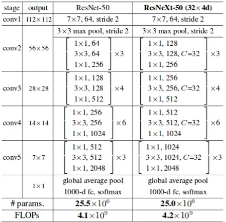
ResNeXt was the first runner up in ILSVRC 2016 with 3.03% top-5 error rate. It is a variant of ResNet. It was built on blocks that aggregate transformations with same topology. ResNeXt worked with parallel independent pathways. It introduced a new dimension called the cardinality which specifies the
[image:5.595.48.273.543.661.2]were obtained when cardinality was increased when compared to results obtained when depth or width were increased. Figure 12 shows the structure of ResNeXt and ResNet blocks. Both the networks contain 5 convolutional layers. They have different widths but the number of parameters remain the same.
Figure 12: The image on the left is a ResNet module & the image on the right is a ResNeXT module with cardinality = 3 [9]
The number and type of layers present in the networks are shown in Figure 13, the networks are similar but the cardinality dimension is added to the ResNeXt network. ResNeXt’s architecture is similar to the architecture of inception model. The main difference between the two is how the outputs from different pathways are used, in ResNeXt they are merged together by simply adding them, while in inception model they are depth concatenated. Both the models use split-transform-merge concept where in the convolutional layers first split the input into different groups of feature maps and then perform normal convolutional and then aggregate the results obtained from each output.
Figure 13: Architecture of ResNet- 50 and ResNeXT-50 networks
DENSENET(2016)
It was developed over the concept proposed in ResNet. Smaller connections are established between layers close to the input and output layers. In DenseNet every layer is linked
[image:6.595.316.526.169.322.2]to every other layer in a feed-forward way unlike the traditional neural network that connects a node to only the nodes in the next layer. The architecture of DenseNet is shown in Figure 14, every layer has inputs from every layer present before it in the network and its feature maps are used as inputs to every layer present after the layer in the network. The layers are very narrow, they contain 12 filters. The important feature in DenseNet is the ability to reuse features extracted in previous layers.
Figure 14: DenseNet Architecture
ResNets adds the outputs of all the feature maps in a layer but DenseNet concatenates them, this process cannot be performed unless all the outputs have same sizes. For the same reason, like the residual module DenseNet works with DenseBlocks that contain layers that work with similar sizes. The network is built over these blocks. Figure 15 shows the blocks arranged together, the layers in between the blocks are transition layers, they change the sizes of the feature maps produced by each block. Since every layer has access to the input and loss function, training the model is easier. All the feature extractions are linked hence same features need not be calculated redundantly. This reduces the number of parameters drastically and reduces the vanishing gradient problem.
Figure 15: Network of blocks [10]
DenseNet outperforms ResNet and produces lesser error rates with relatively fewer parameters. With the increase in parameters the accuracy consistently increases without causing over-fitting which usually happens in regular Convolutional network.
SENET(2017)
SENet or Squeeze and Excitation Networks won ILSCRV 2017. It produced 2.251% top-5 error rate. A convolutional layer has a group of filters which help learn the local spatial connectivity patterns in the
[image:6.595.55.275.465.681.2] [image:6.595.305.524.544.590.2]International Journal of Innovative Technology and Exploring Engineering (IJITEE) ISSN: 2278-3075, Volume-8, Issue-11S, September 2019
These convolutional layers are stacked together in a CNN and this allows them to capture hierarchical patterns with global receptive fields. CNN models that have embedded learning explicitly added to them capture spatial correlations with no extra supervision and this boosts the representation power. SENet focuses on channel relationship, it uses SE blocks or Squeeze and excite blocks that help establish connection between the channels. SE blocks recalibrate channel- wise responses by establishing a connections between channels using feature recalibration. When SE blocks are added to ResNet-50, ResNet’s error rate reduced to 18% which is almost half of the error rate that ResNet produces.
V. PERFORMANCECOMPARISON
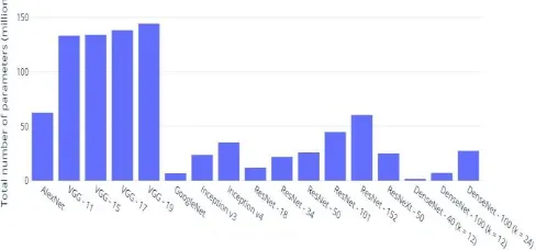
[image:7.595.304.557.64.396.2]The model complexity is the number of parameters that are present in the model. These parameters are weights and biases that are essential in tuning the model for better accuracy. The number of parameters increases with the depth of the model. Figure 16 shows the number of parameters and the model complexity of few of the CNN models. AlexNet contains 75 million parameters that have to be trained. The number next to the model represents the depth or number of layers in the model. VGG-11 contains 11 layers and VGG-19 contains 19 layers. The number of parameters increases from 133 million to 144 million approximately. GoogleNet or Inception v1 model. The number of parameters are important as they specify the amount of memory required by the model. The memory requirement is given in MB. Figure 17 shows the top-1 and top-5 error rates for some important models. All these models are evaluated on a single crop of 224×224. Overall, with the increase in the depth of the model the accuracy increases. But there is a limit for the depth since it can cause over-fitting. The accuracy reduces or reaches a saturation point when this occurs. The top-5 error rate is the percentage of test images for which the actual result or class was not in the top-5 probabilistic classes that the model predicts. Similarly the top-1 error rates is for the top-1 probabilistic class that the model predicts. The models mentioned in Figure 14 are trained on ImageNet and the results are obtained from the official research papers published by the researches themselves. While comparing the models we can see that the error rates have dropped from 15.3% to 3.79% this is lower than the average human prediction that has an error rate of 5.1%.
Figure 16: Number of parameters
Model Top-1 error rate Top-5 error rate
AlexNet 37.5% 15.3%
VGG – 11 29.6% 10.4%
VGG – 15 28.1% 9.4%
VGG – 17 27% 8.8%
VGG - 19 27.3% 9.0%
GoogleNet 32% 6.67%
Inception V3 21.2% 5.6%
Inception V4 20% 5.1%
Xception 21% 5.5%
ResNet – 18 31% 11%
ResNet – 34 26.73% 8.74%
ResNet – 50 24.01% 7.02%
ResNet – 101 22.44% 6.21%
ResNet – 152 22.16% 6.16%
ResNeXt – 50 (32 × 4d)
22.2% 5.9%
DenseNet – 121 25.02% 7.71%
DenseNet – 169 23.8% 6.85%
DenseNet – 201 22.58% 6.34%
[image:7.595.48.292.672.786.2]SENet 18.68% 3.79%
Figure 17: Top-1 and Top-5 error rates
VI. TRANSFERLEARNING
Training a CNN from scratch is difficult, it requires large datasets, high GPU and memory requirement. Many deep learning platforms such as Keras or PyTorch have all the models that are existing in their libraries along with weights. For problem specific tasks or small datasets the concept of transfer learning is suitable. In this an already trained model is used as the start for solving a problem. The base network can be any network that is suitable for our task. The transferability of features from the base model to the required model is explained in detail in [13]. The process improves the model and gradually tunes the model to classify further. The learning process is called inductive transfer where the problem is narrowed down to specific task by reducing the generality. Inductive learning tries to extend the problem and fits the problem to get generalized views. This generalization is not suitable for building task specific CNNs. It searches for solutions using examples and builds a model that is a general solution. Inductive transfer narrows the problem and searches for specific features and problems. Layers are added over the base model to tune the network. The base network we use is the Xception model. There are two parts in this model, the first part is the base model which is the inception model and the second part is the modification or the extra 5 layers over the inception model that makes the model more specific. Freezing the parameters of the inception model uses the whole model while testing and not during training of the model. Building the extra layers is done only using trial and error mechanism, why they work cannot be explained. For the dataset of our choice this works with 1.3% accuracy. The base layer is followed by a normalization layer, pooling layer, dropout layer, and two dense layers. Normalization layer [14] is used to adjust the activation values produced by the inception model. It produces values closer to 0 and strictly below 1. These values are easier to work with in the model and cause lesser computational complexity. Pooling is used to reduce the size of the image output produced by the inception model. Pooling helps to reduce the problem size so that the complexity can be reduced and the model can be efficiently trained. In [15] the authors show how pooling layers improve the model’s efficiency. Drop out layers are very useful, they turn the activation of nodes on and off randomly. Since the dataset is small there might be over-fitting problem, dropout layers help us avoid them. Since the parameters are blocked for some nodes, the other nodes that are causing over-fitting are modified to reduce the weights and biases. The importance of dropout layer is explained in detail in [16]. The dense layer connects all the nodes to all the other nodes in a feed forward fashion. it reduces redundancy in feature detection and reuse of features that have already been detected. they reduce the parameters and are best suitable for small datasets training. The last dense layer is the final classification layer that combines all the features and calculates the probability that the object is of some class. The number of nodes will be equal to the number of classes that the model has to classify into. if the model is of some class it has probability more than 0.5 if the accuracy is okay, and close to 1 if the accuracy of the model is close to
[image:8.595.307.424.116.223.2]100%. The dataset used to train and test the model is from Kaggle. The model is trained for 10 epochs. The breeds of a dog is predicted as shown in Figure 17.
Figure 17: Breed classification
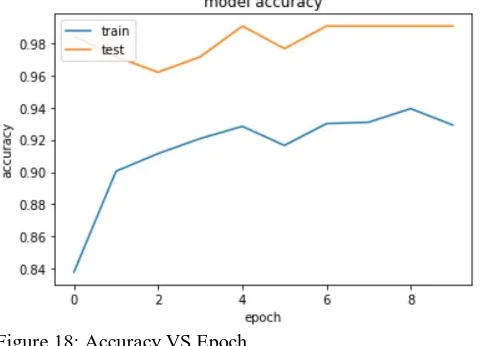
An epoch is one training cycle, a model has to be trained for several epochs to achieve good accuracy. The Figure 18 shows the model accuracy with the number of epochs.
Figure 18: Accuracy VS Epoch
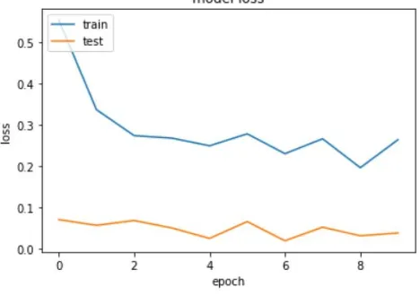
From the graph it can be inferred that for the training data initially the accuracy is low, with the increase in the number of epochs the accuracy increases. After the first epoch the weights and biases are altered to modify the model to increase the probability to match the actual output during this process the accuracy of the system increases. After the fourth epoch the accuracy starts saturating, here there is a slight decrease in it this is due to over-fitting, this can be fixed by including the DenseNets or SENets that reduce the number of parameters. After the model is trained the images are tested. The accuracy of the test images will be high since the model is in its best form. The figure 19 shows the model loss that decreases with the number of epochs. Loss is the error rate this is either takes an top-1 or top-5 error rates. Top-5 error rate is the percentage of images that do not have a prediction in the top-5 for example, if the object is an apple and the system detects the top five classes as apple, orange, ball, sponge and wheel the top-5 assumptions is correct and is not selected. If the prediction does not contain apple then the top-5 error is wrong and the error is added. This process is repeated for all the images in the dataset and the percentage of images for which it is not true are divided by the total number of images in the database. Top-1 is calculated the same way with only the first
[image:8.595.307.547.285.458.2]International Journal of Innovative Technology and Exploring Engineering (IJITEE) ISSN: 2278-3075, Volume-8, Issue-11S, September 2019
saturates as they are inter-linked.
[image:9.595.49.283.106.271.2]Initially the error is high and as the number of epochs increases and the model is further trained the error decreases.
Figure 19: Loss VS Epoch
The same model can be extended to detect more breeds when the right database is created. The overall network accuracy is close to 1.8%. The time taken by the network depends on the complexity of the input image. The top-5 error rate for the same model is 11% which is very less when compared to any regular networks. And the top-1 error rate is 1.8%. If the DenseNets are removed the accuracy drops directly to 80% which is 18% lesser than the network represented here. The number of nodes in the densenet is equal to the number of classes that the model has to classify into. If the image is of some class it has probability more than 0.5 if the accuracy is average, and close to 1 if the accuracy of the model is close to 100%.
VII. RESULTANDCONCLUSION
The introduction of Convolutional Neural Network has changed the way image classification problem has been visualized. The ImageNet competition plays a crucial role in the development of classification algorithms. Recent models outperform humans the error rates of these models are lesser than those produced by humans. From 2010 to 2017 the error rates have dropped from 28% to less than 3% which is a great achievement. Though CNNs take longer time for training, the accuracy is higher than any other classifying algorithm. Improved models take lesser time for training like the ResNets and SENets but produce very accurate results. AlexNet set a new trend in the classification problem by using CNNs. It was followed by the ZFNet, the developers of ZFNet gave a clear pathway to understand the working of CNN. VGGNet another famous model gave insight into the concept that proves the increase in accuracy with the depth of the model. GoogleNet or Inception model used the inception modules to allow parallel working within the system to achieve good efficiency. This was followed by ResNet and ResNeXt that changed the architecture of CNN a little by introducing skip connection that introduced new connections between layers that are not consecutive for solving the vanishing gradient problem. DenseNet increased the accuracy further by connecting all the layers to all the other layers in a feed- forward direction. SENets improved the models further by splitting the channels and giving equal
importance to all of them by parameterizing them. Transfer Learning can be used to build problem specific models instead of creating models from scratch, since creating a new model from scratch will require large GPU capacity and dataset. Layers can be built over an existing model and the output of this base model can be feed into layers stacked up over this model to fine tune the model to recognize differentiating features among the same species.
REFERENCES
1) Y. LeCun, B. Boser, J. S. Denker, D. Henderson, R. E.Howard, W. Hubbard, and L. D. Jackel. Backpropagation applied to handwritten zip
code recognition. Neural computation, 1989.
2) M. D. Zeiler and R. Fergus. Visualizing and understanding convolutional
neural networks. In ECCV, 2014.
3) O. Russakovsky, J. Deng, H. Su, J. Krause, S. Satheesh, S. Ma, Z. Huang, A. Karpathy, A. Khosla, M. Bernstein, et al. Imagenet large scale visual recognition challenge. arXiv:1409.0575, 2014
4) A. Krizhevsky, I. Sutskever, and G. Hinton. Imagenet classification with deep convolutional neural networks. In NIPS, 2012
5) K. Simonyan and A. Zisserman. Very deep convolutional networks for
large-scale image recognition. In ICLR, 2015.
6) C. Szegedy, S. Reed, D. Erhan, and D. Anguelov. Scalable, high-quality
object detection. arXiv:1412.1441v2, 2015.
7) K. He, X. Zhang, S. Ren, and J. Sun. Deep residual learning for image
recognition. In CVPR, 2016
8) S. Zagoruyko and N. Komodakis. Wide residual networks. arXiv preprint
arXiv:1605.07146, 2016.
9) S. Xie, R. Girshick, P. Dollar, Z. Tu, and K. He. Aggregated ´ residual transformations for deep neural networks. arXiv preprint arXiv:1611.05431, 2016.
10) G. Huang, Z. Liu, K. Q. Weinberger, and L. Maaten.Densely connected
convolutional networks. In CVPR, 2017
11) J. Hu, L. Shen, and G. Sun. Squeeze-and-excitation networks.arXiv
preprint arXiv:1709.01507, 2017.
12) D.E. Rumelhart, G.E. Hinton, & R.J Williams. Learning intemal representations by backpropagating errors. In Nature,323:533-536, 1986
13) Jason Yosinski, Jeff Clune, Yoshua Bengio, and Hod Lipson.How transferable are features in deep neural networks? In Advances in Neural
Information Processing Systems, 3320–3328, 2014.
14) S. Ioffe and C. Szegedy. Batch normalization: Accelerating deep network training by reducing internal covariate shift. In ICML, 2015.
15) Scherer, D., Müller, A., Behnke, S.: Evaluation of Pooling Operations in Convolutional Architectures for Object Recognition. In: International
Conference on Artificial Neural Networks, 2010.
![Figure 8: AlexNet architecture [4] The first convolutional layer contains 96 11×11 filters](https://thumb-us.123doks.com/thumbv2/123dok_us/8174769.253129/4.595.45.288.679.751/figure-alexnet-architecture-convolutional-layer-contains-filters.webp)
![Figure 10: Inception module [6]](https://thumb-us.123doks.com/thumbv2/123dok_us/8174769.253129/5.595.63.283.48.143/figure-inception-module.webp)