Lorenzo Gentile
Institute for Data Science, Engineering and Analytics, TH Köln
Köln, Germany [email protected]
Cristian Greco
Aerospace Centre of Excellence, University of Strathclyde Glasgow, United Kingdom
Edmondo Minisci
Aerospace Centre of Excellence, University of Strathclyde Glasgow, United Kingdom [email protected]
Thomas Bartz-Beielstein
Institute for Data Science, Engineering and Analytics, TH Köln
Köln, Germany
Massimiliano Vasile
Aerospace Centre of Excellence, University of Strathclyde Glasgow, United Kingdom [email protected]
ABSTRACT
This paper presents a novel optimisation approach, called Structured-Chromosome Genetic Algorithm (SCGA), that addresses the issue of handling variable-size design space optimisation problems. This is based on variants of standard genetic operators able to handle structured search spaces. The potential of the presented method-ology is shown by solving the problem of defining observation campaigns for tracking space objects from a network of tracking stations. The presented approach aims at supporting the space sec-tor in response to the constantly increasing population size in the around-Earth environment. The test case consists in finding the observation scheduling that minimises the uncertainty in the final state estimation of a very low Earth satellite operating in a highly perturbed dynamical environment. This is evaluated by coupling the optimiser with an estimation routine based on a sequential filtering approach that estimates the satellite state distribution con-ditional on received indirect measurements. The solutions found by employing SCGA are finally compared to the ones achieved using more traditional approaches. Namely, the problem has been reformulated to be faced using standard Genetic Algorithm and another variable-size optimiser, the "Hidden-genes" Genetic Algo-rithm variant.
CCS CONCEPTS
•Mathematics of computing→Mixed-discrete optimisation; •Physical sciences and engineering→Aerospace; • Informa-tion systems→ Uncertainty; •Computing methodology→ Modelling and simulation;
KEYWORDS
Optimisation, Genetic Algorithms, Structured-chromosome, Satel-lite tracking
Permission to make digital or hard copies of all or part of this work for personal or classroom use is granted without fee provided that copies are not made or distributed for profit or commercial advantage and that copies bear this notice and the full citation on the first page. Copyrights for components of this work owned by others than ACM must be honored. Abstracting with credit is permitted. To copy otherwise, or republish, to post on servers or to redistribute to lists, requires prior specific permission and/or a fee. Request permissions from [email protected].
GECCO ’19 Companion, July 13–17, 2019, Prague, Czech Republic © 2019 Association for Computing Machinery.
ACM ISBN 978-1-4503-6748-6/19/07. . . $15.00 https://doi.org/10.1145/3319619.3326841
ACM Reference Format:
Lorenzo Gentile, Cristian Greco, Edmondo Minisci, Thomas Bartz-Beielstein, and Massimiliano Vasile. 2019. Structured-Chromosome GA Optimisation for Satellite Tracking. InGenetic and Evolutionary Computation Conference Companion (GECCO ’19 Companion), July 13–17, 2019, Prague, Czech Re-public.ACM, New York, NY, USA, 9 pages. https://doi.org/10.1145/3319619. 3326841
1
INTRODUCTION
Tracking objects in space has become a major issue for the aerospace community and the general public. Operational satellites require accurate knowledge of their position and velocity to deliver increas-ingly precise services and solid scientific outputs. Non-collaborative objects tracking is needed for collision avoidance and re-entry pre-diction, events which pose a threat respectively to the around-Earth and the terrestrial environment. The continuous growth of the population of artificial objects and small debris orbiting the Earth requires an adequate response in tracking capabilities, schedul-ing, and processing routines. In particular, this necessity applies to the tracking of non-collaborative objects or small missions which cannot rely on dedicated extensive tracking networks.
Therefore, this research develops a scheduling approach to com-pute optimal observation campaigns for a generic object in space. The goal is to improve the knowledge of the object’s state at the end of the tracking window while respecting an allocated budget. As an alternative, the developed approach can also reduce the resources to achieve an accuracy requirement.
A variety of GAs variants for facing variable-sized global optimi-sation can be found in the literature, mostly employed for space tra-jectory design [2, 7, 8]. Of particular interest is the "Hidden-genes" GA (HGGA) adaptation introduced in [2]. In this algorithm, each candidate is represented using all the possible genes and additional "activation genes" indicating which genes have to be considered or when computing the objective and constraint functions. The main drawbacks are that the maximum dimensionality of the prob-lem has to be known a priori and that this is further enlarged by the "activation genes". A more complex, but effective adaptation of GA is proposed in [7, 8]. In these cases, a hierarchical multi-level chromosome structure is adopted in place of the standard "string" one. Defining the concepts of vicinity and hierarchy of genes, the authors introduced a problem formulation that enhanced the exchange of information between chromosomes as well as the computational efficiency in respect to the HGGA. Moreover, this hierarchical formulation can produce a more meaningful exchange of information between chromosomes.
In light of these considerations, we decided to make use of a Genetic Algorithm variant based on hierarchical search spaces and apply it to the problem of generating optimal observation scheduling.
The structure of the paper is the following. Sec. 2 first introduces the general tracking problem and the scheduling formulation, then it presents the specific problem scenario and discusses the cost function. Sec. 3, describes the employed algorithms focusing in particular on the SCGA. The analyses of results are presented in Sec. 4. Finally, final considerations and outlooks of this research are given in Sec. 5.
2
MODEL
This section introduces the model for the scheduling of observations campaigns of space objects from terrestrial ground stations.
First, the generic tracking problem is introduced in Sec. 2.1 in a state estimation probabilistic formulation. Then, the tracking scenario of space objects from ground stations is modelled in Sec. 2.2. The selection of a performance index for quantifying the estimation uncertainty follows in Sec. 2.3. Finally, the specific problem scenario to be used as reference test case is presented in Sec. 2.4.
2.1
Tracking
The system under consideration evolves according to determin-istic ordinary differential equationsf (ODE) describing its state evolutionx(t)in time
xÛ =f(t,x) (1)
x(t0)=x0 , (2)
wherex0is the system initial state at the initial timet0. The state
at later times can be computed by classical numerical integration schemes for ODE.
In real-life scenarios, uncertainty always affects such systems and, therefore, the knowledge of the state at a later timext =x(t). This uncertainty can result from a partial knowledge of the ini-tial state, ambiguously specified model parameters, or unmodelled terms in the equations of motion. Therefore, measurementsytare employed to enhance the knowledge of the system state. Gener-ally, it is not possible to observe the system state directly, and the
measurements are affected by noise. Hence, the state-observation relationship is modelled as
yt =h(t,xt)+ε, (3)
whereε∼ N 0;σy2
is a Gaussian noise with standard deviationσy. The addressed hidden dynamical process is affected by two sources of epistemic uncertainty: the initial state is only partially known, and its uncertainty is modelled with a normal density func-tionp(x0)=N x0;σx20
; the received observationyt is noisy, and its uncertainty is described by a probability distributionp(yt|xt)= N h(t,xt);σy2conditional on the state value.
Given a sequence of observationsy1:l, the tracking problem aims at combining the a priori information about the initial state with the available observations to compute an updated state distribution conditional on the observationsp(xl|y1:l). In Bayesian filtering, this
inference step is formulated by Bayes’ rule [10]
p(xl|y1:l)=p(yl|xl)p(xl)
p(y1:l)
, (4)
where the conditional independence of earlier measurements has been used to simplify the densityp(y1:l|xl)=p(yl|xl). The
condi-tional distribution in Equation (4) is the complete solution of the tracking problem.
However, this update equation has no closed-form solution for general probability distributions. In this work, the inference step is solved using a Square-Root Unscented Kalman Filter (SR-UKF) [14], a sequential filtering approach suitable for normal distributions and non-linear dynamical and observational models. For this sequential scheme, the observations are processed as soon as they are available, and the updated posterior distribution propagated in future until the time of the next measurement. The unscented transform improves the estimation accuracy of standard Kalman Filters for an equal computational burden, whereas the square-root version has more robust numerical stability. The output conditional distribution from the SR-UKF is a multivariate normal distribution described by two parameters, i.e. mean and covariance matrix, as
p(xl|y1:l)=N (xˆl;σx2l) (5)
The smaller are the elements of the covariance matrixσx2lthe more certain is the estimate of the system state.
The described tracking problem is depicted in Fig. 1 for a two-dimensional scenario, where only the first and fourth stations are used to take measurements of the satellite. The ellipses represent the satellite state and its uncertainty in time corresponding to the Gaussian distributions. The colours orange, yellow and green are used respectively for the predicted density, the measurement likelihood, and the filtered distribution.
2.2
Tracking Station Scheduling
It is intuitive to realise that two observation campaignsy1:l,
t0
xg
0= [p0g,v0g]
tf
xp f= [pfp,vfp]
COVg 0
COVp f
Minimise covariance trace
Predicted
Measured
Filtered
Used GS
[image:3.612.55.295.88.189.2]Unused GS Tracking Network
Figure 1: Graphical 2D representation of satellite single pas-sage over network of ground stations. The dark faded blue field-of-view indicates that a station is used to take measure-ment, whereas the light faded blue indicates that the station is not operated. The ellipses symbolise a confidence region of the uncertain state of the satellite. The different colours orange, yellow and green are used to indicate respectively the predicted state, the measurement and the posterior dis-tribution.
Table 1: General free variableui scheme for observation op-timisation.
Description Variable Type Values Use ground stationj Discrete ON/OFF Number of passages to use Integer [0,pmax] ∈N
Indexes of passages to use Discrete [1,pmax] ∈N
Number of observations per passage Integer [0,Nobsmax] ∈N
Times of observations per passage Continuous t∈ [Tin,Tout]pj
In this paper, the challenge addressed is to find the observation campaign which produces the most certain estimate of the satellite final statexf, while respecting a budget constraint, given a net-work of variegated ground stations (GS). The budget constraint is introduced because, in real satellite operations, taking measure-ments from a tracking station has an associated expense, both in terms of human and monetary costs. This constraint prevents the aforementioned extreme case to be a feasible optimum. To further increase the model reality, each tracking station may be charac-terised by specific features depending on its geographical location, and characteristics of the instruments available in loco.
Hence, a station GSjis uniquely specified by defining: its
ge-odetic coordinates, namely latitudelatj and longitudelonj; the measurements modelhj(t,xt); observation covarianceσy2at 90 deg, whereas at lower elevations the covariance elements are assumed to degrade as∼1/sin(El)[11], whereELis the object evelation angle over the local horizon at the observation time. Given such specifications, the object to be tracked may orbit in each station field-of-view (FOV) once, multiple times, or never, depending on the tracking window time-span, station-object relative geometry, and the object initial orbital parameters.
Clearly, it is not possible to pick an observation realisationsyi
directly, but there is an optimisable actionui which influences the measurementyi(ui). In the most general case, the actionui, associated to the ground station GSj, instructs the model whether to
take a measurement from GSjor not, how many, at which passage,
and when in the passage the measurements are to be taken. The variables enclosed in an actionui are summarised in Tab. 1.
Hence, the free variables of the scheduling problem are the se-quence of actionsu1:lthat reduces a performance index on the final
state uncertainty, while respecting imposed budget levels.
2.3
Cost Function
Selecting a performance index which quantifies the accuracy of the filtered state estimate is a non-trivial task [11]. First, since the true state is unknown, a direct measure of the estimation error cannot be computed. Second, each scalar measure would only provide limited information out of the multi-dimensional posterior distribution characterising the state uncertainty.
The Kalman Filter solution returns the Gaussian posterior distri-bution in terms of mean and covariance matrix, which intuitively expresses how spread the density function is. In this work, the trace of the covariance is chosen as performance index to express how confident we are on each element of the state vector. Indeed, although the covariance matrix is usually an optimistic measure, for scheduling purposes only a relative indication of the accuracy between two observation campaigns is needed.
Hence, the scheduling problem can be formally stated as finding the optimal sequence of actionsu1:l that reduces the uncertainty
on the state at the end of the tracking window, conditional on the observations, as
min u1:l J =Tr
σ2
xt xf|y1:l(u1:l) . (6)
Graphically, this performance index corresponds to shrinking the fi-nal orange ellipse in Fig. 1 as much as possible. Being the covariance diagonal composed only of positive terms, the theoretical minimum is zero, i.e. the case of perfect knowledge of the satellite state.
2.4
Reference Scenario
The scenario investigated in this research is characterised by a network of nine ground stations characterised by different geodetic coordinates. Each ground station can take measurements composed of three scalar quantities, namely the relative satellite range, az-imuth, and elevation. The observation covariance atEl=90deg is set as three-dimensional diagonal with elements equal to 1.0e−5.
The satellite to track is in very low-Earth orbit, and the obser-vation window of interest spans from the 2018 October 29 12:00 UTC to the 2018 October 29 20:00 UTC. The initial state estimate in Keplerian elements is
x0=(a[km],e[-],i[rad],Ω[rad],ω[rad],θ[rad])
=(6608.17,1.61e−3,1.685,5.662,1.199,1.589). After conversion to Cartesian coordinates [13], this estimate is the mean of the Gaussian initial state distribution with covariance set as
σ2
x0=diag(1.0e
−2km,1.0e−2km,1.0e−2km,
1.0e−4km/s,1.0e−4km/s,1.0e−4km/s)
[image:3.612.71.277.343.390.2]0 45 90 135 180 225 270 315 90 60 30 0 GS-1 0 45 90 135 180 225 270 315 90 60 30 0 GS-2 0 45 90 135 180 225 270 315 90 60 30 0 GS-3 0 45 90 135 180 225 270 315 90 60 30 0 GS-4 0 45 90 135 180 225 270 315 90 60 30 0 GS-5 0 45 90 135 180 225 270 315 90 60 30 0 GS-6 0 45 90 135 180 225 270 315 90 60 30 0 GS-7 0 45 90 135 180 225 270 315 90 60 30 0 GS-8 0 45 90 135 180 225 270 315 90 60 30 0 GS-9 1st Pass 2nd Pass 3rd Pass 4th Pass 5th Pass 0 45 90 135 180 225 270 315 90 60 30 0 GS-1 0 45 90 135 180 225 270 315 90 60 30 0 GS-2 0 45 90 135 180 225 270 315 90 60 30 0 GS-3 0 45 90 135 180 225 270 315 90 60 30 0 GS-4 0 45 90 135 180 225 270 315 90 60 30 0 GS-5 0 45 90 135 180 225 270 315 90 60 30 0 GS-6 0 45 90 135 180 225 270 315 90 60 30 0 GS-7 0 45 90 135 180 225 270 315 90 60 30 0 GS-8 0 45 90 135 180 225 270 315 90 60 30 0 GS-9 1st Pass 2nd Pass 3rd Pass 4th Pass 5th Pass 0 45 90 135 180 225 270 315 90 60 30 0 GS-1 0 45 90 135 180 225 270 315 90 60 30 0 GS-2 0 45 90 135 180 225 270 315 90 60 30 0 GS-3 0 45 90 135 180 225 270 315 90 60 30 0 GS-4 0 45 90 135 180 225 270 315 90 60 30 0 GS-5 0 45 90 135 180 225 270 315 90 60 30 0 GS-6 0 45 90 135 180 225 270 315 90 60 30 0 GS-7 0 45 90 135 180 225 270 315 90 60 30 0 GS-8 0 45 90 135 180 225 270 315 90 60 30 0 GS-9 1st Pass 2nd Pass 3rd Pass 4th Pass 5th Pass 0 45 90 135 180 225 270 315 90 60 30 0 GS-1 0 45 90 135 180 225 270 315 90 60 30 0 GS-2 0 45 90 135 180 225 270 315 90 60 30 0 GS-3 0 45 90 135 180 225 270 315 90 60 30 0 GS-4 0 45 90 135 180 225 270 315 90 60 30 0 GS-5 0 45 90 135 180 225 270 315 90 60 30 0 GS-6 0 45 90 135 180 225 270 315 90 60 30 0 GS-7 0 45 90 135 180 225 270 315 90 60 30 0 GS-8 0 45 90 135 180 225 270 315 90 60 30 0 GS-9 1st Pass 2nd Pass 3rd Pass 4th Pass 5th Pass
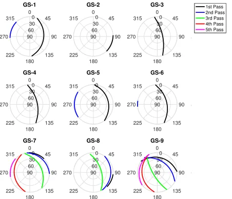
Figure 2: Sky plots of satellite passes over ground stations; the circles correspond to different elevation levels, while the angular quantity indicates the azimuth measured east-wards from the local north. Different colours indicate dif-ferent satellite passes over the same station.
considered is 106.4 in solar flux units, with a mean SRP cross-section of 1.625 m2and a SRP coefficient of 1.3.
Given this scenario, the geometry of this satellite passes above the considered network of tracking stations is visualised in the sky plots shown in Fig. 2, which shows the azimuth and elevation of the satellite when it is over the stations’ local horizon. Hence, the station-satellite relative geometry and the extension of the tracking window determine a number of possible observations windows equal to 21. The best passage over one station’s local horizon is registered for the tracking station GS-9 with an elevation of≈71 deg , which furthermore sees the satellite in five different passes. Stations GS-3, GS-4 and GS-8 see the satellite with decent elevation angles≥50 deg, while the worst passages are realised over stations GS-2 and GS-5. Therefore, it can be predicted that an optimal schedule would take measurements from stations which see the satellite at higher elevation angles, as in the model the observation covariance degrades when the elevation decreases.
Generally, the more observations are used the more reliable the computed estimate is, hence the lower the value of the cost func-tion will be. As discussed, this new informafunc-tion comes at a cost in a real-life scenario. For this reason, the maximum number of measurements will be imposed as a constraint and varied over the different runs. In order to quantitatively assess the impact of the maximum available number of the observations over the uncer-tainty in satellite tracking, the analysed optimisation strategies have been repeated varying this in a range from 15 to 65 with the span of 5. These values are representative of an operative mission scenario that would benefit more from the employment of the proposed algorithm.
3
OPTIMISATION PROBLEM
This section introduces the methodologies adopted for minimis-ing the uncertainty associated with the state of an object in space varying the scheduling of the observation campaign. The opti-misation strategies, as well as the problem formulations, will be described and compared in detail. In this research, the proposed Structured-Chromosome Genetic Algorithm (SCGA) is compared to the standard Genetic Algorithm and an implementation of the "Hidden-genes" Genetic Algorithm (HGGA). All of them have been used for minimising the uncertainty associated with the state of the satellite at the end of the tracking window.
The optimal resources allocation for the object’s tracking is the common aim of all the optimisers employed but, as will be shown in the following sections, the problem formulations are different. In particular, a throughout explanation of the proposed optimiser and its problem formulation is given in section 3.2 and the others are summarised in section 3.1.
3.1
Standard GA and "Hidden-genes" GA
The performances of the proposed optimiser have been compared to the ones of a standard Genetic Algorithm [5] and the HGGA variant proposed in [2] . As well known, the standard GA is not suitable for handling variable-sized optimisation problems. Therefore, applying this strategy for facing the presented problem requires making assumptions on the maximum dimensionality. In this particular problem, this entails assuming that the GSs are always used. If that, the quantity to be managed by the optimiser is limited to the budget for measurements at each satellite pass over the GSs. This assumption, in theory, should not tragically compromise the strategy’s capability of optimally allocating the budget but, as the results will show, extremely harden the task.
The HGGA makes use of activation genes for activating or de-activating genes. As in the previous case, it is assumed that the GSs are used at every pass so the dimensionality of the problem is the greatest possible. Then, at every gene an "activation" one is associated. Its value indicates whether to consider or not the asso-ciated gene in the decision space. By means this trick, it is possible to encode and manage solutions with different architectures using standard genetic operators.
In the scenario considered, the maximum number of decision variables is 21, one for each time the satellites falls in the FOV of one of the GS composing the tracking network. In the standard GA problem formulation, these constitute the complete decision space whereas, in the HGGA one, the 21 additional activation genes are introduced.
Two different implementations of the HGGA have been tested. In one the crossover operator performs a one-point crossover acting at one on the overall chromosome (original+activation genes) in the second, this is applied separately on the decision and activation genes as proposed in [2] .
3.2
Structured-Chromosome Genetic
Algorithm
3.2.1 Problem Formulation. The adopted problem formulation
aims at condensing the information in the free variables (see Tab. 1) making use of the concept of hierarchy for enhancing the operators capability of reaching good performing solutions. One of the main advantages of this problem formulation is that it is not required assuming a priori the number of ground stations to use and the number of passes in which these are activated. This implies that the characteristics of the candidate observation campaign are contained in a flexible number of decision variables.
In this problem formulation, the search space has been struc-tured in a hierarchical way imposing dependencies between genes. Consequently, the target of the operators is not a single gene but rather an entire gene structure. This structure is actively helping the operators to perform "meaningful" transformations over the candidates. In fact, it helps to preserve the overall information lim-iting the extrapolation of one gene from its context. Due to the elevated interactions, blindly exchanging genes might lead to a high information destruction rate.
Differently from classical genetic algorithms, in SCGA a chro-mosome (solution) is represented by a matrix either indicating the value of the gene either its position in the hierarchy of the chromo-somes. The genes are grouped intogene classesthat characterise them by data type, dependent genes, and bounds. For the observa-tion scheduling optimisaobserva-tion, the hierarchical structure is stratified in three levels.
The gene classGround Stationforms the top of the hierarchical structure. The value of this gene indicates the number of different satellite passes in which the specific ground station will be em-ployed to measure the satellite state. Thus, given that the modelled GS network is constituted by nine ground stations, nine genes be-longing to this class are present in all the solutions, one for each GS. However, the limiting upper bound of these genes is determined by the referring GS. In fact, sown in Fig. 2, every GS has the satellite in its FOV a different number of times. So the genes belonging to the gene classGround Stationdon’t have all the same bounds.
The gene classOrbit index (OI) constitutes the second level of hierarchy. This variable specifies the index of the pass of the satellite in the FOV of the associated GS to allocate the budget for measurements specified by the subordinated gene classBudget for Measurements(BfM). Obviously, a one-to-one correspondence between the bounds assigned toGround StationandOrbit index
genes has to exist.
As mentioned, as a rule of thumb, the more the observations the more reliable the estimate should be. To simulate a real-life scenario, a cost associated to each observation has been introduced to simu-late the restrictions of a real observation campaign. Consequently, a
Table 2: Decision variable of the Observation Scheduling op-timisation Problem.
Gene Type Lower Bound Upper Bound
Ground Station Integer 0∀GS19 [2,1,1,1,2,1,5,3,5] Orbit index Discrete 1∀GS19 [2,1,1,1,2,1,5,3,5]
Budget Real 0∀GS19 1∀GS91
budget limitation constraining the number of observations has been imposed and it has been varied into the independent runs in order to have a quantitative indication of its effect on the uncertainty in the final state estimation.
TheBudget for Measurementsgene class indicates the percentage of the total available budget allocated for a set of measurements performed by a given GS at a given pass of the satellite in its FOV. The relation between the decision variables in the optimisation
Budget for Measurementsand the value requested by the model
Number of Measurementsis expressed by the equation:
NoM=
$
B f M Cost
%
(7)
whereNoMis theNumber of MeasurementsandB f Mthe allocated
Budget for Measurements. This indirect measure of the number of measurements has been preferred in the perspective of testing the proposed approach assigning different levels of reliability and sen-sibility to the measurements of every GS. Accordingly, the unitary cost of the measurements by different GSs will also differ. In this experiment, for the sake of simplicity, the same unitary cost has been assigned to each GS.
3.2.2 The algorithm.The adopted algorithm is a
population-based heuristic optimiser that relies on two operators to pursue the search of the global optimum: the crossover and the mutation. These operators, nowadays established in stochastic fixed-length mixed-discrete optimisation, have been redefined in order to manipulate candidates characterised by different length and structure. Then, these strategies are integrated into the classical structure of genetic algorithms [5]. In the following, a throughout explanation of the most relevant aspects of the proposed operators will be given.
3.2.4 Selection.In stochastic optimisation the way candidates are selected is crucially important. This, greatly affects the veloc-ity of convergence towards a region, determining the balance be-tween exploration and exploitation of the search space. This step is strongly dependent on the method used for fitness assignment. The fitness shall reflect the "goodness" of a candidate orienting the selection to the most promising chromosomes. In the observation scheduling optimisation problem the objective function can assume a wide range of values that can differ in 7 order of magnitude or even be impossible to compute because of model divergence. In light of this, it has been decided to use ranking fitness assignment filtering the objective function differing less than 3 order of magnitude from the best of the current population. For selecting the chromosomes for crossover, the Tournament selection with tournament size equal to 6 has been used. In addition, the best 10% members of the popula-tion are preserved immutably. This can sometimes have a dramatic impact on performance by ensuring that the algorithm does not waste time re-discovering previously found solutions.
3.2.5 Crossover. The crossover is an operator that exchanges
genes between two different chromosomes (parents) to produce two new candidates (children). This aims at combining and transferring the information contained in the parents to the children. In such a way, hopefully, the children will contain the relevant characteristics that originated the performance of their parents.
In classical fixed-size algorithms, all the genes lie on the same level and have a well-defined position and meaning. Genes in the same positions in the strings of two different chromosomes repre-sent the same variable. This is not the case for structured chromo-somes. Here, swapping genes among parent chromosomes on the basis of their position may result in selecting genes that represent different variables and creating unfeasible and meaningless solu-tions. Hence, a different strategy for selecting genes to swap based on their class has been proposed by [7].
The crossover operation is permitted only on genes belonging to the same class. This approach guarantees a semantically correct crossover where the picked gene, as well as the dependent genes, are swapped. Furthermore, the adopted crossover operator aims at maximising the information exchange per crossover operation. However, in the preliminary stage of this research, the strategy proposed in [7] has been used but appeared to be too destructive, making the information contained in the parents disappear over the generations. For this reason, a revised one has been developed. In this, the number of exchanging genes belonging to each class is computed in regards to the structure of the two parents chromo-somes. This helps to homogenise the crossover operation all over the hierarchy of the chromosome. Moreover, the already swapped genes are removed from the list of eligible genes for crossover. This helps to prevent the repetition of the crossover operation on the same genes that would reduce the exchange of information. It is worth to mention that, although the crossover on genes related to the same GS andOIis encouraged, the probability of exchanging of information between uncorrelated genes is preserved. The feasibil-ity then is not guaranteed and the candidates are always checked and, if needed, repaired. The procedure adopted is then able to create meaningful children that respect the hierarchical structure of the parents. However, the respect of bounds or constraints is
not guaranteed and a step of repair is necessary for evaluating the response of the candidates.
3.2.6 Mutation.The mutation operator is characteristic of most of the population-based optimiser. Many different variants of this operator can be found in literature for standard fixed dimension optimisation [3]. As in the case of the crossover, a new mutation operator has been introduced to deal with structured chromosome. In this case, two main steps can be recognised in the mutation op-eration. First, the mutation of the chosen gene to be mutated and in particular its value, then, treating the context of the mutated gene. The former finds many similarity points with the standard mutation operators. Indeed, it aims essentially at perturbing the current value of the gene in order to introduce randomness in the chromosomes’ evolution. In the problem of tracking observation campaigns deter-mination, variables of different types have to be managed. Hence, the basics of the mutation operations described in [4] have been borrowed to be used as gene variable perturbation operators. The mutation of the offspring relies on operations acting differently on real, integer and discrete variables, all respecting the requirements for a mutation strategy in the search spaces: Accessibility, Feasi-bility, Symmetry, Similarity, ScalaFeasi-bility, and Maximal Entropy [4]. The operator achieves this by adding normally distributed noise to real-valued variables. For integer variables, the distribution is based on the difference of two geometrical distributions. Categori-cal variables are simply re-sampled (uniform randomly) with some probability. The probability and the magnitude of mutation are controlled by hyperparameter, thestrategy parameters, that evolve during the optimisation in a self-adaptive fashion. To each candi-date, a set of hyperparameter is associated. This is initialised as described in Alg. 1 and evolves undergoing the same crossover operations of the associated chromosome. However, the crossover operation for the mutation hyperparameter consists in simply av-eraging the hyperparameter sets associated to the chromosomes selected by the operator. Hence, the mutation strength itself is also governed by an evolutionary process. The philosophy behind self-adaptation is that the evolutionary process can solve two problems simultaneously: the determination of the best strategy variables, and the determination of the best object variables.
The second step of the mutation consists in treating the depen-dent genes. In particular, their value has to undergo the mutation operation and their number has to be consistent with the new value assumed by the higher-level gene. For better clarify the process, the pseudocode of the mutation is reported in Alg. 2.
In this case as well, the respect of all the constraints is not guar-anteed. Then, the repair function is employed to guarantee feasible solutions.
3.2.7 Repairing.For ensuring candidates feasibility after the
input:Chromosomes,LB,UB;
NGenesPerType←average number of type of the genes in
the chromosomes;
τ =√ 1
2·NGenesPerType;
ρ= 1
q
2·√NGenesPerType ;
σcontinuous =(U B−LB) ×0.1;
σinteдer =(U B−LB) ×0.33 ;
σcateдor ical =0.1 ;
Algorithm 1:Initialisation of the mutation hyperparameters for Observation scheduling optimisation. The global learning rates are denoted byτ, the local learning rate byρand step sizes byσ.
theOrbit index genes are removed to be maximum the number of times the satellites falls in the ground station’s FOV and their values are modified in order to minimise the difference between the unfeasible and the feasible solution. The second operation aims at identifying and correcting theOrbit indexgenes that don’t respect the semantic constraints. In example, whether moreOrbit index
genes refer to the same satellite’s pass or whether anOrbit index
gene refers to an unfeasible satellite’s pass. Finally, the algorithm checks whether the budget limit is exceeded. If this happens, all theBfMare scaled to be have an overall used budget equal to the maximum allowed.
4
RESULTS
The developed tool is tested in a quasi-realistic scenario for the tracking of a satellite in a very low Earth orbit (LEO), where the dynamics is highly nonlinear, as presented in Sec. 2.4.
Three optimisation strategies have been tested on the satellite tracking observation campaigns problem: the standard GA, the HGGA with the one-point and two-points crossover, the SCGA with adaptive mutation, and the SCGA with mutation hyperparameters fixed to the initial ones. Specifically, these algorithms have been tested varying the maximum number of possible measurements in a range from 15 to 65 with a span of 5. For each configuration 5 independent runs have been run in order to have more statistically significant results.
All the optimisation runs have been limited to 500 generations,his results in 13503 function evaluations for the SCGA,and 15000 for the others algorithms.
The results in all the problem configurations are summarised in Fig. 3 where the covariance trace of the final optimal solutions found in the different runs is depicted by means box plots. For all the budgets, the GA is significantly outperformed by the others. This straightens the hypothesis that traditional fixed-size optimi-sation strategies actually struggle to face variable-size problems, even when they have been reformulated. To compare the other algo-rithms, the Conover’s rank-based pairwise multiple-comparison [1] tests have been used. These tests indicate that there is no signifi-cant difference between all the other algorithms’ performance. For further considerations, a visualisation of the best-found solutions in the configuration with the maximum number of measurements = 25 has been reported in Fig. 4. From this Figure, it can be seen that
input:geneToMutate,σ,τ,ρ,LB,UB;
genesPresence←lenдths(genesPerClass);
for i∈geneToMutatedo
дeneClass←geneClass of i;
ifgene type ofiis realthen
дeneV alue←
дeneV alue+σдeneClass·N(0,1) · (U B−LB);
дeneV alue←max(дeneV alue,LBдeneClass);
дeneV alue←min(дeneV alue,U BдeneClass);
end
ifgene type ofiis integerthen
NGene←genePresenceдeneClass;
p← N Gene·σσ
дeneCl ass;
p← 1−p
1+√1+p2;
p←max(p,1e−3);
G1←rдeom(NGene,prob=p);
G2←rдeom(NGene,prob=p);
дeneV alue←дeneV alue+(G1−G2) · (U Bi−LBi);
дeneV alue←max(дeneV alue,LBi);
дeneV alue←min(дeneV alue,U Bi);
end
ifgene type ofiis categoricalthen
Activation=N(0,1)>σдeneClass;
ifActivationthen
дeneV alue←pick one random possible feasible
value
end end
ifihas dependent genesthen
ifnumber of dependent genes has to be changedthen ifgenes have to be addedthen
initialise new dependent genes
end
ifgenes have to be removedthen
randomly pick dependent genes to be removed
end end
Mutate all the dependent genes
end end
fori∈geneClassdo
NGene←дenePresencei;
ifgene type ofiis real or integerthen
σi ←max(1,σi ·eτi∗N(0,1)+ρi∗N(0,1));
end
ifgene type ofiis categoricalthen
σi ← 1
1+(1−σiσi)·eτi∗N(0,1)+ρi∗N(0,1);
end end
1e−01
1e−02
1e−03
1e−04
25 30 35 40 45 50 55 65 70 75 85
Maximum number of observations
Co
var
iance tr
ace (log scale)
[image:8.612.55.295.84.214.2]Optimisers hidden−One−Point hidden−Two−Points SCGA−Adaptive SCGA−Static standard−GA
Figure 3: Box-plots of representing the best results found by all the algorithms in all the analysed problem’s configura-tions. 75 2 1 2 3 2 4 3 GS−1 GS−2 GS−3 GS−4 GS−5 GS−6 GS−7 GS−8 GS−9 Obj [1e−5] 92 1 1 3 2 1 5 GS−1 GS−2 GS−3 GS−4 GS−5 GS−6 GS−7 GS−8 GS−9 Obj [1e−5] 101 1 1 1 3 2 1 GS−1 GS−2 GS−3 GS−4 GS−5 GS−6 GS−7 GS−8 GS−9 Obj [1e−5] 107 2 3 2 4 1 GS−1 GS−2 GS−3 GS−4 GS−5 GS−6 GS−7 GS−8 GS−9 Obj [1e−5] 156 1 1 1 3 2 1 3 2 1 GS−1 GS−2 GS−3 GS−4 GS−5 GS−6 GS−7 GS−8 GS−9 Obj [1e−5] standard−GA 15 1 1 3 3 2 19 1 1 3 2 5 4 3 2 1 20 1 1 3 2 3 2 3 2 1 21 1 1 3 1 4 2 1 23 1 1 1 1 4 3 3 2 1 hidden−One−Point 15 1 1 3 3 2 1 17 1 1 1 3 3 2 23 1 1 1 3 1 3 5 1 23 1 1 4 3 2 1 3 4 2 1 24 1 1 4 2 1 3 5 3 hidden−Two−Points 12 1 1 1 3 2 4 3 18 1 1 3 3 2 1 18 1 1 3 3 2 1 19 1 1 3 1 3 2 22 2 1 1 3 3 2 1 SCGA−Adaptive 19 1 1 3 2 3 2 20 1 1 3 3 2 21 2 1 3 4 2 21 1 1 1 1 3 4 1 21 1 3 3 2 1 SCGA−Static No.Meas
Visualization of the best solutions || No.Meas= 25
2 4 6 8 10 No.Meas
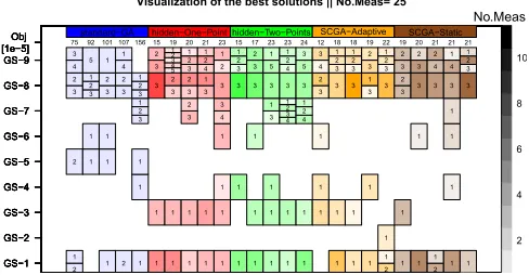
Figure 4: Visualisation of the best solutions found with the maximum number of measurements=25. On the vertical axis, theJvalue and theOrbit indexesat which every GSs is used are reported. The colour shades represent the budget al-located to the specific observation: the darker the more mea-surements employed. The colour indicates the optimiser em-ployed.
the solutions found by the standard GA differ significantly from the ones found by the competitors: the standard GA does not make use of all the available budget, and only the observation campaigns found by the standard GA employ the GS-5 that is one of the two (with GS-2) with the lowest elevation angle.
The solutions found by the HGGA and the SCGA are also inter-esting. Notably, one of the convenient stations for the early part of the tracking window, GS-1 and GS-3, are employed in almost all solutions whereas, for the late part, both the high elevation ones GS-8 and GS-9 are always employed. However, Fig. 4 shows great variability in the selected orbit indexes and the budget allocation, that reveals a high multimodality and complexity of the search space.
Finally, the impact of the maximum number of measurements can be addressed by comparing the uncertainty in the final state for the best solutions when varying this parameter. This has a strong influence on the configurations with small budgets, whereas it appears to vanish with the growth of the available budget.
The results indicate that only the variable-size optimisers are able to find and select the most important features while discarding the bad characteristics.
5
CONCLUSIONS
This paper presents a novel strategy, Structured-Chromosome Ge-netic Algorithm, that aims at tackling variable-size design space optimisation problems advantaging of the concept of genes hierar-chy.
This algorithm has been applied for solving the problem of au-tonomously generating optimal satellite tracking observation cam-paigns under a limited budget. This concerns the aerospace com-munity as nowadays the presence of objects orbiting the Earth is being pushed to the limit. Enhancing the efficiency of the ob-servation schedules aims at making the tracking of space objects sustainable for the future. The presented scheduling formulation re-quires to optimise the sequence of observations in order to improve the knowledge of the satellite position and velocity at the end of the tracking window. Each observation results from a free action associated with each tracking station in the considered network. Such observations are processed using the SR-UKF to compute the posterior distribution of the state uncertainty, by efficiently merg-ing different sources of information, namely the prior knowledge, the dynamics, and the measurements. The trace of the associated covariance matrix has been selected as performance index to syn-thetically measure the uncertainty associated with each component of the satellite state.
The proposed method has been tested on a quasi-realistic sce-nario in which nine ground stations were available to track a satel-lite in very low Earth orbit. For comparison, the standard GA and the "Hidden-gene" GA have been run on the same test case. The in-fluence of the budget on the uncertainty in final state estimation as well on the searching algorithms’ performance has been addressed by varying the number of available measurements.
The results indicate that the presented methodology can suc-cessfully enhance resources allocation strategies in space object tracking problems if compared to traditional approaches. How-ever, the limited number of repetitions made, the complexity and the apparent deceptiveness of the objective function make further analyses absolutely needed for a definitive claim.
The SCGA has been implemented to work with any dynamic, measurement model and station network such that different test cases can be tested in future. The apparent parity of the SCGA and "Hidden-genes" GA performances can be partially due to the simplicity of the problem formulation. In the authors’ opinion, introducing additional features such like a cost associated to the measurements dependent by the GS employed or differentiating the GSs by their accurateness could accent the SCGA’s capacity of handling complex problem formulations. A further possible outlook of this research would be the definition of a similarity measure in order to embed this optimiser in a Surrogate model-based optimi-sation framework. Finally, a real-time approach that employs this observation schedule as first guess could be developed to improve the solution optimality in online applications.
ACKNOWLEDGMENTS
[image:8.612.53.297.259.386.2]REFERENCES
[1] William Jay Conover and Ronald L Iman. 1979. On multiple-comparisons proce-dures.Los Alamos Sci. Lab. Tech. Rep. LA-7677-MS(1979), 1–14.
[2] Shadi A Darani and Ossama Abdelkhalik. 2017. Space Trajectory Optimization Using Hidden Genes Genetic Algorithms.Journal of Spacecraft and Rockets55, 3 (2017), 764–774.
[3] Imtiaz Korejo and Shengxiang Yang. 2012. Comparative Study of Adaptive Muta-tion Operators for Genetic Algorithms. Inin MIC 2009: The VIII Metaheuristics International Conference, 2009. 196 Journal of Emerging Technology and Advanced Engineering Website: www. ijetae. com (ISSN 2250-2459, Volume 2, Issue 2. Citeseer. [4] Rui Li, Michael TM Emmerich, Jeroen Eggermont, Thomas Bäck, Martin Schütz,
Jouke Dijkstra, and Johan HC Reiber. 2013. Mixed integer evolution strategies for parameter optimization.Evolutionary computation21, 1 (2013), 29–64. [5] Melanie Mitchell. 1998.An introduction to genetic algorithms. MIT press. [6] Oliver Montenbruck and Eberhard Gill. 2012.Satellite orbits: models, methods
and applications. Springer Science & Business Media.
[7] Hui Meen Nyew, Ossama Abdelkhalik, and Nilufer Onder. 2012. Autonomous Interplanetary Trajectory Planning Using Structured-Chromosome Evolutionary Algorithms. InAIAA/AAS Astrodynamics Specialist Conference. 4522. [8] Hui Meen Nyew, Ossama Abdelkhalik, and Nilufer Onder. 2015.
Structured-chromosome evolutionary algorithms for variable-size autonomous interplane-tary trajectory planning optimization.Journal of Aerospace Information Systems
12, 3 (2015), 314–328.
[9] Julien Pelamatti, Loïc Brevault, Mathieu Balesdent, El-Ghazali Talbi, and Yannick Guerin. 2017. How to deal with mixed-variable optimization problems: An overview of algorithms and formulations. InWorld Congress of Structural and Multidisciplinary Optimisation. Springer, 64–82.
[10] S. Sarkka. 2013.Bayesian Filtering and Smoothing(1st ed.). Cambridge University Press, New York.
[11] Bob Schutz, Byron Tapley, and George H Born. 2004.Statistical orbit determination. Elsevier.
[12] Luca Scrucca et al. 2013. GA: a package for genetic algorithms in R.Journal of Statistical Software53, 4 (2013), 1–37.
[13] D. A. Vallado and W. D. McClain. 2007. Fundamentals of Astrodynamics and Applications(3rd ed.). Springer, New York.