Development of an extended mean value engine model for predicting
1
the marine two-stroke engine operation at varying settings
2
Gerasimos Theotokatos
a,1,
Cong Guan
b,1,*, Hui Chen
b, Iraklis Lazakis
a3
a Department of Naval Architecture, Ocean & Marine Engineering, University of Strathclyde, 100 4
Montrose Street, Glasgow G4 0LZ, UK 5
b Key Laboratory of High Performance Ship Technology of Ministry of Education, School of Energy 6
and Power Engineering, Wuhan University of Technology, 1178 Heping Road, Wuhan 430063, China 7
* Corresponding author. 8
1 These authors contributed equally to this work. 9
Abstract This study focuses on the development of an extended MVEM capable of predicting the
10
engine performance parameters (thermodynamic, flow and mechanical) of two-stroke marine engines 11
at varying settings of injection timing and turbine area. The extension employed mapping of a number 12
of the engine parameters carried out based on a zero-dimensional model. Both the zero-dimensional 13
and the mean value engine models were developed in MATLAB/Simulink environment following the 14
same modular approach and their accuracy was validated against experimental data from shop trials. 15
Subsequently, the zero-dimensional model was used for engine parametric simulation by changing the 16
start of fuel injection and the turbocharger turbine area. By analyzing the derived results, the 17
relationships between the investigated engine parameters were established and the appropriate 18
corrections were applied in the MVEM. The extended MVEM was benchmarked against the 19
zero-dimensional model and MVEM at steady and transient conditions and the derived results were 20
analysed and discussed revealing the advantages and limitations of the investigated modelling 21
approaches. Based on the obtained results, the proposed extension methodology improves the MVEM 22
prediction capability without considerably increasing the complexity and the execution time and 23
investigations overcoming limitations of the MVEM. 1
Key words Extended mean value engine model; Zero-dimensional model; Marine two-stroke diesel
2
1. Introduction
1
The large two-stroke marine diesel engine is widely used for propulsion of the vast majority of 2
vessels in the last few decades due to its high efficiency and reliability. In order to attain improved fuel 3
efficiency and achieve environmentally cleaner operation, engine manufacturers have developed 4
electronically controlled versions of marine diesel engines [1,2]. In these, the computer-controlled 5
high-pressure hydraulic systems with advanced sensors, actuators and control valves have been used to 6
replace the camshaft that exists in traditional engine versions for adjusting the fuel injection timing and 7
exhaust valve opening/closing. Additionally, turbochargers with variable geometry turbines and exhaust 8
gas waste gate valves have been applied for increasing the engine efficiency throughout the whole 9
engine operating envelope especially at low load conditions. Furthermore, recently turbocharging 10
systems with two-stages have been investigated for implementation in marine engines in order to 11
simultaneously increase efficiency and reduce NOX emissions [3,4]. For reducing SOX emissions, two
12
alternative measures have been proposed and used [5]; these include either the engine operation by 13
using a low sulphur fuel or the installation of a scrubber in the engine exhaust pipe. Low sulphur heavy 14
fuel oil (LSHFO), marine gas oil (MGO) and natural gas stored in liquefied form (LNG) are the 15
alternative proposed for immediate implementation by the maritime industry stakeholders, whilst other 16
alternative fuels including methanol, ethanol and hydrogen are proposed for future usage. 17
As the development of a large two-stroke marine diesel engine is time consuming and costly 18
procedure, various engine modelling techniques have been used for investigating the engine 19
steady-state performance and transient response as well as for testing the alternative design of the 20
engine systems. In the current literature, different model types have been reported to predict engine 21
models [26 ,27 ]. As the modeling complexity increases, i.e. from transfer function models to 1
computational fluid dynamic models, the representation of the engine working process is improved, but 2
at the same time a greater execution time and amount of input data are required, so that the model 3
becomes more laborious. As the MVEMs are a compromise between the simpler transfer function 4
models and the more detailed zero- or one-dimensional models, these are widely used in investigations 5
that include the development and design of the engine control systems, where a fast execution time and 6
model simplicity are needed [6,28,29]. The MVEMs employ a limited amount of input data and 7
reasonable execution time whilst predicting the engine behaviour with adequate accuracy, whereas their 8
drawbacks include their inability to predict the in-cycle variation (e.g. per degree of crank angle) [6] 9
and as a result the engine brake specific fuel consumption (BSFC) and efficiency under different 10
settings (e.g. varying start of injection timing, turbine area and exhaust gas bypass, etc.). In the cases 11
where in-cylinder parameters are required, the zero- or one-dimensional models can be used. For the 12
case where the estimation of engine performance at varying settings is of interest [ 30 ], the 13
zero-dimensional models seem to be the appropriate option. Furthermore, for adequately predicting 14
emissions, two-zone or multi-zone combustion models are required along with the appropriate 15
emissions kinetics mechanisms, which further increase the model complexity and the running time 16
[31,32], thus rendering the zero-dimensional models application quite challenging for cases that require 17
simulation of engine transients for long periods, varying engine settings and control system design [6], 18
for example, ship maneuvering predictions [33] or system components control [34]. 19
Theotokatos [12] reported the MVEM categories and the development of a modular MVEM in 20
MATLAB/Simulink environment. The advantages and drawbacks of two different approaches were 21
also discussed based on previously published data. Dimopoulos et al. [35] included the diesel engine 22
marine energy system simulation platform called COmplex Ship Systems MOdelling and Simulation 1
(COSSMOS), providing the users with the flexibility to select the desired ones according to the 2
intended application. Nikzadfar et al. [36] introduced an extended MVEM for control-oriented 3
modeling of diesel engines transient performance and emissions by utilizing Artificial Neural Networks 4
(ANN) to mimic the engine cycle thermodynamic model. The applied neural network technology 5
requires a large number of data sets to capture the in-cylinder process with desired level of accuracy, 6
and besides that the amount of data increases significantly if emissions are to be modelled. Nielsen et al. 7
[34] simplified the original mean value engine model by removing the non-dominant dynamics and 8
developed a control-oriented model of the oxygen fraction in the scavenge air manifold. This model 9
can be used effectively for the engine control system design but cannot provide the engine performance 10
predictions at varying engine settings as it still has to confront the mean value engine model limitations. 11
Fadila and Charbel [37] developed an extension of MVEM and in-cylinder single zone model for high 12
speed four-stroke diesel engine dedicated for Hardware in the Loop (HIL) applications. The model only 13
includes the air system, combustion system, exhaust system and fuel system without considering the 14
turbocharger and propeller, which means it cannot be regarded as a full engine model. In addition, a 15
quad core Real Time Processor Computer (RTPC) is needed in order for the in-cylinder extended 16
model to be run in real time. Extending the modular MVEM reported in Theotokatos [12], Baldi et al. 17
[38] proposed a combined MV-0D approach applied for a large marine four-stroke diesel engine, where 18
the zero-dimensional model was used for representing the closed cycle of one engine cylinder and the 19
mean value engine model employed for simulating the open part of the cycle as well as for the other 20
engine components. Nevertheless, the zero-dimensional model needs to be called at each time step 21
engine model calculation speed by estimating the cylinder exhausting and scavenging processes as 1
linear functions and abandoning engine cylinder cycles at certain intervals. This hybrid model can be as 2
fast as the MVEM for the steady state conditions in that the boundaries of every cylinder cycles remain 3
the same, however the calculation speed is improved at the expense of the engine performance 4
prediction precision during the dynamic process. 5
Although hybrid modelling approaches offer an acceptable execution time, the engine control 6
systems design applications require simpler models as even limited zero-dimensional modelling 7
introduces complexity [6,34]. In order to capture the engine performance at varying settings with 8
reasonable execution time, an effective approach is to use a MVEM coupled with lookup tables or 9
response surfaces representing the engine cylinders parameters variation, which can be derived from 10
the zero-dimensional model parametric runs. In this respect, the advantages of the MVEMs, i.e. the 11
modularity and low execution time, along with the more accurate prediction of engine performance 12
parameters at varying settings that zero-dimensional models provide can be exploited. A similar 13
modelling approach was used in Livanos et al. [40,41] for designing and testing control schemes for an 14
ice-class tanker propulsion plant system. The used engine model included lookup tables derived by 15
using a calibrated zero-dimensional model parametric runs, and the in-cylinder engine performance 16
parameters were estimated by using linear interpolation. However, as this is a case-dependent approach 17
of modelling marine engines, an extended MVEM based on analytical expressions can provide an 18
additional advantage and more flexibility as it could capture both the flow and mechanical parameters 19
variation. This is a novel element of the present study as there is not reported a general approach for 20
extending the MVEM by applying the corrective formulae to the respective parameters. As the 21
electronically controlled versions of marine engines become more popular and new components that 22
(EGR) and turbocharger cut-out valves are used nowadays, this extended mean value engine model is 1
an alternative for providing both adequate accuracy and fast running times with reduced modelling 2
complexity. Besides that, the extended MVEM can be used to predict with fidelity the engine operation 3
under different conditions without requiring re-calibrations of the model parameters for representing 4
engine with varying settings. 5
The proposed extended modelling approach was employed herein to investigate a large two-stroke 6
engine performance prediction with varying start of injection (SOI), turbine area and exhaust gas 7
bypass settings. The model was benchmarked against the zero-dimensional model and MVEM, and the 8
simulation results were used to discuss its advantages and drawbacks against the other two modelling 9
approaches. 10
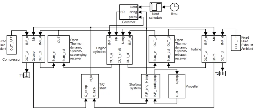
2. Models description
11
The zero-dimensional and mean value engine models used in this work were previously developed 12
by the authors in MATLAB/Simulink environment following a modular concept. The zero-dimensional 13
model has been described in detail in Guan et al. [30] where it was used for the prediction of a two-stroke 14
large engine performance at slow steaming conditions. The MVEM was described in detail in 15
Theotokatos [12]. The models structure is shown in Fig. 1. Each part of the engine is represented by a 16
block that exchanges variables with the adjacent blocks through the appropriate connections. The models 17
use a number of elements including flow elements, receivers, mechanical elements (shaft and load) and 18
control element (PI governor). For both models, the scavenging and exhaust receivers are considered to 19
be flow receiver elements (control volumes), whilst the turbocharger components (compressor and 20
turbine) are represented as flow elements. Fixed fluid elements of constant pressure and temperature are 21
and turbocharger shaft rotational speeds. The engine governor element, which is used to adjust the engine 1
fuel rack position, is considered to be of the proportional-integral (PI) type and incorporates the 2
appropriate fuel rack limiters, whereas the propeller element is used for calculating the propeller torque. 3
The thermodynamic properties of the working medium either air or gas are considered to be functions of 4
temperature, pressure and fuel-air equivalence ratio [42]. 5
The flow elements use as input variables the pressure, temperature and the properties of the 6
working medium contained in the adjacent elements (flow receiver(s) or fixed fluid), whereas their 7
output variables include the mass and energy flow rates entering and exiting the flow element as well 8
as the absorbed (for the case of compressor) or produced torques. The mass and energy flows are 9
provided as input in the adjacent flow receiver elements, whereas the torques are required as input in 10
the shaft elements. The output of turbocharger shaft element, i.e. the turbocharger speed, is provided to 11
the compressor and turbine elements. The output of the crankshaft element includes the engine and 12
propeller rotational speeds; the former is supplied as input to the engine cylinders and engine governor 13
elements, whereas the latter is advanced in the propeller element. 14
The difference between the zero-dimensional model and MVEM lies in the cylinder block. The 15
zero-dimensional model cylinder block is more comprehensive as it simulates the closed cycle process 16
(compression, combustion and expansion) by using a one-zone approach, and the scavenging process by 17
employing a two-zone approach [30]. The zero-dimensional model cylinder block uses as input the 18
scavenging ports and exhaust valves profiles as well as the fuel variable injection timing. On the 19
contrary, the MVEM cylinder block is simpler and the flow is calculated by using an equivalent orifice 20
approach whereas the cylinder performance parameters are calculated by using algebraic equations. 21
2.1 Zero-dimensional model
The cylinders are modelled as flow receiver elements using either the open or closed 1
thermodynamic systems consideration depending on their operating phase (open cycle or closed cycle, 2
respectively). For calculating the cylinder working fluid thermodynamic parameters, the mass and 3
energy conservation laws as well as the ideal gas state equation in each considered control volume zone 4
are used [43-45]. Assuming that the system can be characterized by using the temperature, mass, 5
pressure and equivalence ratio, the one zone model employs three first-order differential equations for 6
calculating the temperature, the mass and the burnt fuel fraction along with the ideal gas equation for 7
calculating the pressure and algebraic equations for estimating the working fluid properties. The two 8
zone scavenging model (the first zone includes air whereas the second zone includes exhaust gas) 9
employs six first-order differential equations for calculating the temperature and the mass for each zone, 10
the burnt fuel fraction of the second zone and the cylinder pressure in conjunction with the algebraic 11
equations for calculating the working medium properties. 12
The Woschni-Anisits combustion model [45] is used for describing the combustion process. This 13
model employs a simple Wiebe function, the shape factor and the combustion duration of which are 14
calculated by using a reference point respective values along with the combustion air/fuel equivalence 15
ratio and engine speed. In this respect, the model constants need to be calibrated for one operating point 16
as the model adjusts the model parameters in other operating points. The Woschni model [46] is 17
employed for calculating the cylinder gas to wall heat transfer coefficient with the default value being 18
as proposed for large two-stroke engine. For the estimation of the engine friction losses, an equation 19
providing the engine friction mean effective pressure as a function of the cylinder maximum pressure 20
and the average piston speed is used [47]. When all the engine cylinders are considered to be identical, 21
and provided as input for the calculation of engine crankshaft rotational speed. The combustion model 1
constants in the zero-dimensional model are given in Table 1. 2
3
2.2 Mean value engine model
4
The engine cylinders block is regarded as a flow element in the MVEM. The air mass flow rate 5
entering the cylinder is calculated considering the equivalent of two consecutive orifices, each one 6
representing the cylinders scavenging ports and exhaust valve. The mass flow rate of the exhaust gas, 7
exiting the engine cylinders, is estimated by using the continuity equation adding the mass flow rates of 8
the air entering the engine cylinders and the injected fuel. The latter is calculated using the number of the 9
engine cylinders, the engine rotational speed and the injected fuel mass per cylinder and per cycle, which 10
is regarded as a function of engine fuel rack position. A critical parameter for the MVEM set up and 11
calibration is the fuel chemical energy proportion in the exhaust gas (ζ), which represents the working 12
medium energy flow change across the cylinder (increase of the energy flow of the air entering the 13
cylinders) as fraction of the fuel energy released within the combustion chamber [6,45]. Thus, the 14
parameter ζ can be used to calculate the energy flow rate exiting the engine cylinders element according 15
to the following equation: 16
_ _ _ _
e e cyl d a a cyl u comb f L
m h m h
m H (1) 17Previous studies [6,45] showed that the parameter ζ can be approximated as a linear function of 18
the engine brake mean effective pressure (BMEP) [48]: 19
1 2
k k BMEP
(2)20
Typically, ζ is calculated and calibrated for each load using available engine performance data 21
measured during the engine trials or provided by the engine manufacturer [49]. As the parameterζ is 22
overcome this limitation, the extension of the MVEM is proposed herein. 1
The indicated mean effective pressure is calculated as the product of the rack position, the 2
engine maximum indicated mean effective pressure and the combustion efficiency, which, in turn, 3
is regarded as a function of engine air to fuel ratio [44]. The friction mean effective pressure that 4
includes all the engine mechanical losses is considered a function of the indicated mean effective 5
pressure and the engine crankshaft speed according to [6,12]. The engine brake mean effective 6
pressure is calculated by subtracting the friction mean effective pressure from the indicated mean 7
effective pressure, whereas the engine torque is calculated using the brake mean effective pressure 8
and engine cylinders displacement volume [43]. 9
3. Models validation
10
The two-stroke marine diesel engine MAN Diesel & Turbo 7K98MC steady state operation was 11
simulated by using both the zero-dimensional model and the MVEM developed in MATLAB/Simulink 12
environment. The engine is of the cross-head type and turbocharged by using the constant pressure 13
turbocharging system concept equipped with three turbocharger units. One air cooler unit is installed 14
downstream each compressor in order to cool the hot compressed air. In addition, three electric driven 15
blowers are used for providing adequate air flow when the engine operates at loads below 40%. Each 16
blower receives the air exiting the respective engine air cooler unit and discharges that to the engine 17
scavenging air receiver. The blowers are activated when the engine air scavenging receiver pressure 18
becomes lower than 1.55 bar, whereas they are switched off for pressure values greater than 1.7 bar. 19
The main engine characteristics as well as the required input data were taken from the engine 20
manufacturer project guide [50]. The engine steady state performance data were obtained from the 21
Both models were set up by providing all the required input data, which included the engine 1
geometric data, the turbocharger compressor and turbine performance maps, the engine ambient 2
conditions, the constants of engine model equations and the propeller loading. The exhaust valves and 3
scavenging ports profiles as well as the fuel injection timing are needed for the zero-dimensional model. 4
The above required data was collected by using the engine project guide [50], whereas the compressor 5
and turbine maps were available from authors previous work [11]. Initial conditions are also required 6
for the variables that are calculated by integrating differential equations, i.e. the engine/propeller shaft 7
and turbocharger shaft rotational speeds as well as the pressure and temperature of air and gas 8
contained in the engine receivers. The engine three turbocharger units as well as the installed air 9
coolers and blowers were considered to have identical performance. 10
To validate both models simulation runs under steady state operating conditions at 25%, 50%, 75% 11
and 100% of the engine MCR load were performed, as these loads were investigated in the official 12
engine shop tests. The percentage error between the predicted engine performance parameters and the 13
respective shop trial data of both models are given in Table 3. It can be inferred that both models 14
predictions exhibit sufficient accuracy for the high engine load region and the engine operation at low 15
loads (down to 25% load). Therefore, both the engine zero-dimensional model and MVEM are 16
considered to provide satisfactory accuracy and can be used with fidelity for investigating the engine 17
operation. 18
Apart from the simulation of the official shop tests engine operating points, additional simulation 19
runs were conducted at 10%, 15%, 20%, 30%, 35%, 40% and 85% load, respectively. A set of the 20
predicted engine performance parameters including the receivers pressures and temperatures, the 21
temperature of the exhaust gas exiting the engine, the turbocharger speed, the brake specific fuel 22
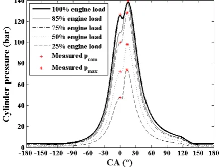
and compression pressure (for zero-dimensional model) is presented in Fig. 2. The respective 1
parameter values obtained from the engine experimental data from shop trials for the engine loads 25%, 2
50%, 75% and 100% are also shown in Fig. 2. Despite the fact that the MVEM cannot predict the 3
in-cylinder parameters, the two models seem to provide satisfactory predictions covering the whole 4
engine operating region. The cylinder pressure diagrams derived by using the zero-dimensional model 5
at 25%, 50%, 75% and 100% engine loads are presented in Fig. 3. 6
The minimum value of the brake specific fuel consumption is observed at 85% load, at which the 7
fuel injection timing is the most advanced leading to the most advanced combustion start as it can be 8
deduced from the pressure diagrams shown in Fig. 3, resulting in almost the same cylinder maximum 9
pressure value as the one in 100% load. Due to the activation of the engine blowers, discontinuities in 10
the engine performance parameters variations are observed between 35% and 40% load. The blower 11
activation results in a greater air flow entering the engine cylinders and thus increases the air to fuel 12
ratio. Therefore, the temperature of the exhaust gas contained in the engine receiver and the 13
temperature of the gas exiting turbine reduce approximately 42 K compared to their respective values 14
at 40% load (where the blowers are not activated). In addition, at engine loads 35% and lower, the 15
scavenging air receiver temperature increases around 5 K compared to the respective value of 16
approximately 302 K at 40% load. This is attributed to the blower compression process, which results 17
in air temperature rise. At 25% engine load, the exhaust gas temperature slightly increases due to the 18
fact the engine air to fuel ratio reduces since the compressor operates at lower speed. At 20% engine 19
load and lower, there is a decrease in the exhaust gas temperature, which is attributed to the fact that the 20
fuel amount injected to engine cylinders is reduced more drastically in comparison with the respective 21
4. Extension of MVEM based on zero-dimensional model results
1
In this section, the extension of the MVEM is described. This involves the following steps: 2
a) Mapping of the engine performance parameters based on the zero-dimensional model; 3
b) Derivation of the analytical equations for the identified model parameters corrections; 4
c) Incorporation of the derived equations to the MVEM; 5
d) Validation of the extended MVEM based on various case studies. 6
4.1 Mapping and analysis of engine performance parameters based on zero-dimensional model
7
As inferred by Guan et al. [30], the MVEM cannot predict the engine performance at varying 8
settings including changes of the fuel injection timing and the turbine area. Thus, the zero-dimensional 9
model was used to map the engine performance parameters representing the engine operation at varying 10
settings. 11
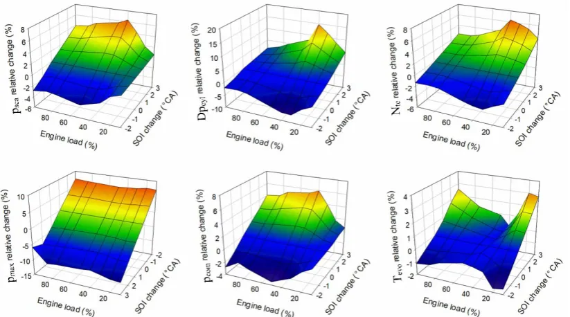
4.1.1 SOI change
12
First, changes of SOI in the range from -2 to +3°CA were considered for various engine loads from 13
10% up to 100% of MCR. The resulting relative changes of the engine performance parameters at each 14
load were calculated using as basis the parameters reference values shown in Fig. 2, which were 15
calculated considering the respective reference fuel injection timing values. The calculated engine 16
performance parameters variations as function of the SOI change and engine load are presented in Fig. 4. 17
Discontinuities can be observed at the region of 40% load owing to the blowers activation. It can be 18
clearly inferred from Fig. 4 that the SOI variation affects in a lesser or a greater extent the engine 19
performance parameters depending on the engine load. The engine parameters that are influenced most 20
significantly at around 40% load region are the scavenging receiver pressure, the cylinder pressure drop 21
as the cylinder compression pressure. The cylinder temperature at exhaust valve open (EVO) is affected 1
in a lesser extent at this load point, whereas the SOI variation effect on the cylinder maximum pressure 2
remains comparable at all loads. The cylinder pressure drop exhibits a maximum relative change of 15%, 3
whilst the other engine parameters are influenced much less with the observed maximum relative change 4
being at around 6%. 5
In order to show more noticeably the influence of SOI on the in-cylinder pressure, the variation of 6
calculated engine cylinder pressure and heat release rate diagrams as a result of SOI change at 75% load 7
is presented in Fig. 5. From Fig. 5(a), it can be observed that as expected the SOI retard results in a 8
significant reduction of the cylinder maximum pressure accompanied with an increase of the exhaust gas 9
temperature during the expansion phase including EVO point (not shown in Fig. 5). As it is well reported 10
in the literature, this is due to the fact that the SOI retard shifts the combustion process towards the 11
expansion phase (as can be also inferred from Fig. 5(b)), thus a proportion of the fuel energy is added 12
later into the cylinder working fluid. A slight increase of the cylinder compression pressure at 75% load 13
is observed with the SOI retard as shown in Fig. 5(a), which is attributed to the increase of the scavenging 14
receiver pressure (as can be inferred from Fig. 4). This is due to the fact that the SOI retard leads to a 15
higher exhaust gas temperature so that the greater available exhaust gas energy increases the 16
turbocharger speed and eventually the scavenging receiver pressure. The SOI retard also leads to a higher 17
specific fuel consumption as shown in Fig. 7, which will be presented later on in this section, as the lower 18
cylinder maximum pressure and the higher cylinder compression pressure result in a lower engine brake 19
power and therefore, a greater fuel amount is needed for obtain the same brake power. From the 20
preceding discussion it is inferred that the well-known behaviour of the engine parameters caused by 21
The parameter ζ is used in the mean value engine model to represent the fuel chemical energy 1
proportion in the exhaust gas entering the turbine as it was introduced in Equation (1). This parameter is 2
very critical for the model calibration and the prediction of the exhaust receiver temperature and as a 3
result, the other engine performance parameters. The parameter ζ was calculated according to Equation 4
(1) by using the derived zero-dimensional model results, in specific, the energy flow of exhaust gas 5
exiting the cylinder, the energy flow of air entering the cylinder, the combustion efficiency, the fuel mass 6
flow rate and the lower heating value. The relative variation of ζ as function of the SOI change and 7
engine load is presented in Fig. 6. The relative change of the parameter ζ (from the baseline value used 8
for the calculation as presented in Fig. 2) takes values in the range from -0.02 to 0.035 with the SOI 9
change spanning from -2 to +3°CA. It can be inferred that the fuel chemical energy proportion in the 10
exhaust gas at the turbine inlet increases with the SOI retard as well as the overall ζ relative change 11
follows a monotonic trend. 12
By applying surface fitting using the MATLAB curve fitting tool, it was found that the following 13
equation can be used to represent the ζ relative change as function of the SOI change (in degrees CA) and 14
the engine load fraction: 15
1 2 3
S O I k k L k S O I S O I
(3) 16
The obtained R-square value was above 0.99, which indicates that the derived equation successfully 17
captured the involved parameters correlation. 18
The engine brake specific fuel consumption at these settings was also predicted using the 19
zero-dimensional model; its relative change was plotted as function of the SOI change and the engine 20
load as shown in Fig. 7. As explained above, the SOI retard results in the reduction of the maximum 21
cylinder pressure, which consequently, increases the engine brake specific fuel consumption. The BSFC 22
in Fig. 2) are in the range between -0.015 to 0.034 with the SOI change being from -2 to +3°CA. 1
Similarly to the SOI influence in the relative change of ζ, the BSFC relative change follows a monotonic 2
trend with the fuel injection timing change and the engine loads. In addition, the BSFC is more sensitive 3
to the SOI influence as the engine load increases. 4
The following equation was derived to represent the BSFC relative change as function of the SOI 5
change and the engine load. By comparing Equations (3) and (4), it can be deduced that both ζ and BSFC 6
relative changes follow similar functions with load and SOI change. The calculated R-square value was 7
also above 0.99. 8
1 2 3
S O I
B S F C k k L k S O I S O I
(4) 9
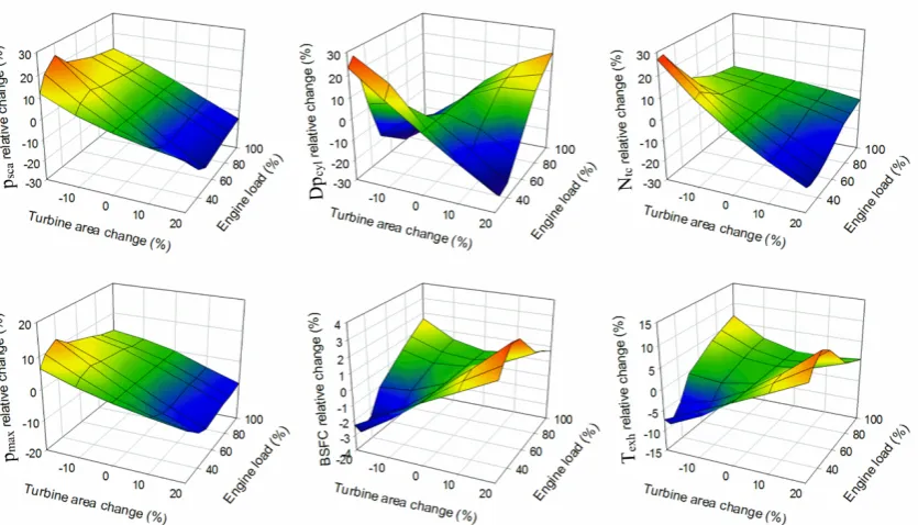
4.1.2 Turbine area change
10
Subsequently, the turbine area change influence on the engine performance parameters was 11
investigated. Simulation runs were performed by applying changes of the turbine area between -20% and 12
+20% at engine loads from 25% to 100%using the zero-dimensional model. The engine performance 13
parameters relative changes at each load were calculated considering the baseline values (shown in Fig. 14
2) derived by using the reference turbine area. The calculated engine performance parameters variations 15
as function of the turbine area change and the engine load are presented in Fig. 8. The performance 16
parameters reference values at each load are calculated from the zero-dimensional model steady state 17
results without blower activation in order to decouple the blower influence. 18
It can be inferred from Fig. 8 that the engine parameters including the scavenging receiver pressure, 19
the cylinder pressure drop and the turbocharger speed are most significantly affected by the turbine area 20
change with an observed maximum relative change at 30% (much higher than the ones of the other 21
the maximum cylinder pressure. However, the reduction of BSFC becomes less distinctive at the 1
ultra-low load region since the turbocharger speed is too low to ensure sufficient air flow. At loads above 2
75%, the reduction of turbine area causes the engine cylinders air flow restriction (as it is deduced by the 3
considerable reduction of the cylinder pressure drop), which has as a result the decrease of the engine 4
efficiency, thus increasing the BSFC. 5
A very detailed description of the engine operation with turbocharger cut-out (equivalent to the 6
reduction of turbine area) can be found in the authors’ previous works [11,30], where it was concluded 7
that when turbine area changes are employed, the MVEM has the capability of predicting the engine 8
performance parameters variation apart from the brake specific fuel consumption. This is because of the 9
MVEM limitation on representing the in-cylinder process, on the contrary to the zero-dimensional 10
model. As it can be inferred from Fig. 8, the scavenging receiver pressure is greatly influenced by the 11
change of turbine area. The scavenging air receiver increase results in the BSFC reduction as well as in 12
lowering the engine thermal loading as more air is trapped into the engine cylinders. Based on the 13
zero-dimensional model results, the relative variation of the BSFC as function of the scavenging receiver 14
pressure relative change and the engine load was derived and shown in Fig. 9. The one turbocharger unit 15
cut-out operation was also included as it follows the same trend as the case with reduction of turbine area 16
and thus, it can be considered as the extreme condition of the turbine area variation. The relative change 17
of the BSFC was found to be between -0.06 and 0.07, whilst the relative change of the scavenging 18
receiver pressure lies in the range -0.2-+0.43. 19
By applying curve fitting, it was found that the following Equation (5)can be used to represent the 20
BSFC relative change as function of the scavenging receiver pressure relative change and the engine load 21
in the case of variable turbine area: 22
1 2 3 ,
,VGT sca VGT sca VGT
BSFC k k L k p p
(5)
The scavenging receiver pressure relative change in the case of variable turbine area used in 1
Equation (5) is calculated based on the scavenging receiver pressure values (psca,ref) shown in Fig. 2, as
2
follows: 3
, ( , , ) / , sca VGT sca VGT sca ref sca ref
p p p p
(6)4
where psca,VGT is the calculated scavenging receiver pressure for the case of turbine area change.
5
The R-square for this correlation was calculated approximately 0.97, which indicates an adequate 6
prediction of the used non-linear curve fit. 7
The derived coefficients values for the investigated slow speed two-stroke diesel engine are 8
provided in Table 4. In this respect, the proposed extension methodology could be generalised and 9
applied during the MVEM set-up process. However, this requires further validation, which is out of the 10
scope of the present work. 11
4.2 Incorporation of the derived corrective equations in the MVEM
12
Since the fuel chemical energy proportion in the exhaust gas entering the turbine as well as the 13
engine brake specific fuel consumption with varying SOI settings cannot be predicted by the MVEM, 14
appropriate corrections need to be employed. 15
Firstly, the ζ correction to capture the dependency on the SOI change is applied in the MVEM by 16
using the following equation: 17
1 0
(1 ) ( )(1 )
r ef S O I k pz b kz S O I
(7)
18
where ζref denotes the ζparameter for the reference engine operation (without including varying settings
19
of SOI and turbine area). 20
Secondly, the BSFC correction to capture the dependency on the SOI change is subsequently 21
mean effective pressure is insignificant, as follows: 1
, / (1 ) ,max / (1 )
i i ref SOI R i comb SOI
p p
BSFC F p
BSFC (8)2
where pi ref, denotes the indicated engine mean effective pressure for the reference engine operation.
3
Equations (7) and (8) in conjunction with Equations (3) and (4) conclude the correction procedure 4
for the case of the SOI change. In addition, the steps described below are applied for the case where 5
simultaneous turbine area and SOI changes are used. 6
As the engine brake specific fuel consumption with varying turbine area cannot be predicted by the 7
MVEM, the correction of the indicated mean effective pressure needs to be employed similarly to 8
Equation (8), by estimating the BSFC relative change according to Equation (5). Since the fuel injection 9
timing also influences the scavenging receiver pressure (variation up to 6% as can be inferred from Fig. 10
4), the scavenging receiver pressure reference values (psca,ref) used in Equation (6) should be modified.
11
The new reference pressure (psca,SOI,ref) is estimated by using the initial reference values (psca,ref from Fig.
12
2) and their relative change values (∆psca,SOI shown in Fig. 4), according to the following equation:
13
, , , (1 , )
sca SOI ref sca ref sca SOI
p p
p (9) 14The scavenging receiver pressure relative change variation in the case of SOI change (∆psca,SOI) as
15
function of the SOI change and the engine load (presented in Fig. 4) was analysed by using the MATLAB 16
curve fitting tool. Due to the fact that the blowers were activated below the 40% engine load point, a 17
piecewise function was applied to capture this parameter variations. It was found that the similar 18
formulae (as provided in Equations (3)-(5)) can be used to correlate these three variables at both above 19
and below the 40% engine load with the calculated R-square values being 0.9937 and 0.9837, 20
respectively. In addition, an interpolation function was used to smooth the transition in the range between 21
30% and 40% loads. 22
varying SOI can be derived using the following piecewise function: 1
1, 1 2
2
, 0.4
( 0.3) / 0.1 , (0.4 ) / 0.1 , 0.3 0.4
, 0.3
sca SOI
f SOI L L
p L f SOI L L f SOI L L
f SOI L L
(10) 2 where: 3
1 , 1 2 3
f SOI L k k L k SOI SOI
4
2 , 4 5 6
f SOI L k k L k SOI SOI
5
The values of the constants in Equation (10) are provided in Table 5. 6
For the case that only turbine area change is employed, ∆psca,SOI equals to zero and therefore, the
7
scavenging receiver pressure baseline values used for the turbine area change correction (psca,SOI_ref in
8
Equation (9)) are the same as the respective initial reference values (psca,ref shown in Fig. 2).
9
Finally, the indicated mean effective pressure is corrected by using the following equation: 10
,max / (1 )
i R i comb SOI VGT
p F p
BSFC
BSFC (11) 11It can be inferred from Equation (11) that the applied BSFC corrections affect the calculated 12
indicated mean effective pressure, and as a result the brake mean effective pressure. Therefore, the rack 13
position calculated by the engine governor model will be different in the predictions of the original 14
MVEM and the extended MVEM. Thus, for the same engine operating point, different amount of fuel 15
and as a result a different value of BSFC will be calculated. In summary, the extension of MVEM can be 16
readily applied following the proposed correction procedure, the flowchart of which is illustrated in Fig. 17
10. 18
5. Case studies
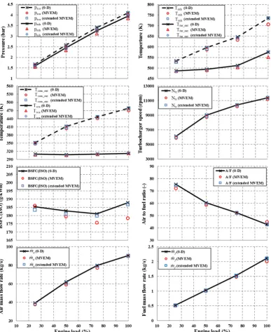
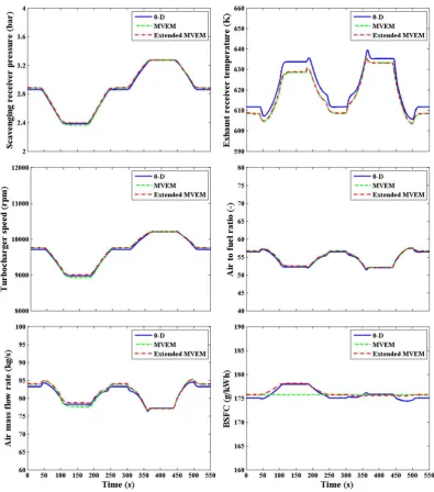
19
In order to examine the extended MVEM capability of accurately predicting the engine 20
area reduced by 20% at 25%, 50%, 75% and 100% engine loads was investigated. The predicted engine 1
performance parameters from the zero-dimensional model, the original MVEM as well as the extended 2
MVEM are shown in Fig. 11. The validated zero-dimensional model is considered to provide the 3
baseline predictions. 4
Retarding the SOI results in the increase of the exhaust temperature and the fuel consumption as 5
explained above, whereas reducing the turbine area decreases the exhaust temperature and the fuel 6
consumption at low load region as can be seen from Fig. 8. Therefore, their combinatory effect on the 7
engine performance parameters depends on the specific conditions. In comparison to the normal engine 8
operation (shown in Fig. 2), the considered settings substantially increase the receiver pressures and 9
turbocharger speed at all loads resulting in lower predicted exhaust temperature at loads below 50% and 10
higher at loads above 50%. Additionally, the fuel injection timing influence on the receiver pressures, the 11
turbocharger speed as well as the exhaust temperatures becomes more significant as the engine load 12
increases. 13
As it can be observed in Fig. 11, the original MVEM lacks the capability of predicting the BSFC 14
with changing either the SOI or the turbine area. The calculated BSFC values from the original MVEM 15
are very close to the ones derived from the reference engine operation as shown in Fig. 2, exhibiting 16
considerable errors in comparison with the respective results of the other two models. As load increases, 17
the SOI retard influence on the BSFC becomes more considerable. The engine cylinder cycle becomes 18
less efficient as explained above and therefore, the predicted BSFC values are considerably greater than 19
the ones in the normal operation. 20
The ζ correction renders the extended MVEM adequate for accurately predicting the exhaust gas 21
temperature in the engine receiver and the turbine outlet, whereas the BSFC correction (eventually 22
The relative errors between the extended MVEM and zero-dimensional model are in the range of 0.5 to 1
1.0% for the BSFC and 0.05 to 1.03% for the other parameters, which reveals the fact that all the main 2
engine parameters derived from the extended MVEM and the zero-dimensional model match well. Thus, 3
the proposed MVEM extension approach with corrections for fuel injection timing and turbine area is 4
considered to be effective. The predicted fuel mass flow rate deviations between the original MVEM and 5
the other two models are not so noticeable due to their relatively small values, but they actually follow a 6
consistent variation trend similar to the BSFC one, which is expected since the BSFC is calculated 7
considering the fuel mass flow rate and the engine brake power. The original MVEM predictions exhibit 8
errors in the range 0.4-5.1% for the BSFC and 0.2-3.9% for the other parameters, and therefore, it needs 9
to be used with caution for the investigation of the engine performance in cases of engine varying 10
settings. 11
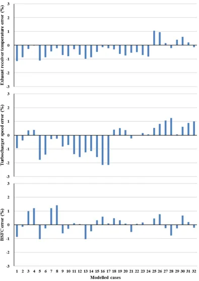
Moreover, to test other engine settings, different combinations of SOI and turbine area changes as 12
shown in Table 6 were considered. It should be noted that the extended MVEM applied all the 13
corrections and values presented in Table 4. The validated zero-dimensional model was used to provide 14
the required reference values. The predicted results were compared with the corresponding ones obtained 15
by using the zero-dimensional model and the derived relative errors are presented in Fig. 12. The engine 16
settings included the SOI advanced and retarded by 2°CA along with the turbine area changes of -20%, 17
-10%, +10% and +20% at 4 different loads (25%, 50%, 75% and 100%). So totally 32 combination 18
cases were investigated as presented in Table 6. It can be observed from Fig. 12 that the deviations of the 19
main engine parameters in the most cases are less than 1% and the highest deviation is 2.1%, which 20
demonstrates that the extended MVEM predictions are accurate enough and the model can be used for 21
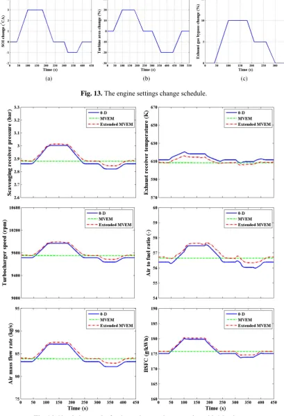
examine the extended MVEM prediction accuracy with varying engine settings at transient operation. 1
The following three engine settings change schedules were defined at 75% engine load in order to test the 2
models response: (a) the start of fuel injection ramp changes shown in Fig. 13 (a); (b) the turbine area 3
change percentage ramp variation (between -20% and +20% the normal turbine area) shown in Fig. 13 4
(b); (c) the exhaust gas bypassed by the waste gate ramp changes (compared to the normal exhaust gas 5
amount) presented in Fig. 13 (c). A set of the derived simulation results including the scavenging air 6
receiver pressure, the exhaust gas receiver temperature, the turbocharger speed, the air to fuel ratio, the 7
air mass flow rate and the BSFC, is presented in Fig. 14-16 using the zero-dimensional model, the 8
original MVEM as well as the extended MVEM. 9
As the original MVEM does not handle the varying fuel injection timing, its predicted values for all 10
the engine parameters almost remained constant as can be observed from Fig. 14. The extended MVEM 11
results sufficiently match the ones of the zero-dimensional model, although slight steady deviations are 12
observed with the maximum error being at 0.81%. Based on the derived results, it can be concluded that 13
the extended MVEM can capture the engine performance variation with the SOI changes at transient 14
operation. 15
As already explained above, the original MVEM can be used to simulate the engine behaviour but 16
cannot adequately predict the BSFC variation with the turbine area changes. This can be also easily 17
inferred from Fig. 15 where it is observed that the original MVEM derived results are very similar with 18
the results of the other two models except for the BSFC. The extended MVEM can capture the engine 19
performance variation with the turbine area changes including the BSFC changes at transient operation 20
as its predictions match the ones of the zero-dimensional model with the maximum error being found to 21
be 0.92%. 22
comparable to the effect of VGT. This can be also observed from the results presented in Fig. 16. It can 1
be inferred that the extended MVEM adequately predicts all the engine performance parameters with 2
the exhaust gas bypass changes (the maximum error is 0.75%), thus improving the MVEM predictive 3
capability. Therefore, it can be concluded that the extended MVEM can be used with fidelity to 4
investigate the engine operation with exhaust gas bypass. 5
From the above analysis, it was proved that the extended MVEM has the capability of predicting 6
the engine performance parameters (power, speed, BSFC, efficiency), the working medium states 7
(pressure and temperature, air to fuel ratio), the flow parameters (flow rates), and turbocharger 8
parameters (speed, pressure ratio, efficiency) in both steady state and transient conditions. 9
The three models running time on a standard personal computer with Intel Core i7-2600 processor 10
for the preceding three investigated cases was examined and the results are shown in Table 7. It can be 11
inferred from that the extended MVEM requires around double execution time in comparison with the 12
original MVEM due to the incorporation of the corrective equations, whereas it is still approximately 7 13
times faster than real time and 570 times faster than the zero-dimensional model. It should be noted 14
that the zero-dimensional model included blocks for all the engine cylinders; much less execution time 15
is expected in case where one cylinder is only modelled and the other cylinders parameters are 16
calculated by considering each cylinder phase angle. Although the MATLAB/Simulink environment 17
offers the platform for an effective development and set-up, implementation of the zero-dimensional 18
model in MATLAB or another programming language considerably reduces the models execution 19
time. 20
6. Conclusions
21
derived by using the curve fitting of a detailed zero-dimensional model parametric runs results. The 1
engine performance parameters variations were thoroughly analysed at varying SOI and turbine area 2
settings using the zero-dimensional model. The extended MVEM was benchmarked against the 3
zero-dimensional model and the original MVEM. The main conclusions derived from this work are 4
summarized as follows. 5
The engine parameters in specific, the scavenging receiver pressure, the cylinder pressure drop, the 6
turbocharger speed and the cylinder compression pressure, are influenced most significantly by the SOI 7
variation at around 40% load region; however, the cylinder temperature at EVO is affected in a less 8
extent at this load point whereas the SOI variation effect on the cylinder maximum pressure remains 9
comparable at all loads. The cylinder pressure drop exhibits a maximum relative change of 15%, whilst 10
the other engine parameters are influenced much less, with the observed maximum relative change being 11
at around 6%. The SOI retard shifts the combustion process towards the expansion phase resulting in a 12
significant reduction of cylinder maximum pressure accompanied with an increase of the exhaust gas 13
temperature at EVO, which eventually leads to higher BSFC. As the SOI changes are from -2 to +3°CA, 14
the parameter ζ relative change was found to vary in the range of -0.02 to 0.035, whereas the BSFC 15
relative change was calculated between -0.015 and 0.034. Furthermore, both the overall ζ and BSFC 16
relative changes follow a monotonic trend with various fuel injection timings and engine loads. 17
The effects of turbine area change on the engine parameters including the scavenging receiver 18
pressure, the cylinder pressure drop and the turbocharger speed are the most significant with an observed 19
maximum relative change at 30%. At engine loads lower than 75%, the turbine area reduction results in 20
an increase of the scavenging receiver pressure and as a result the maximum cylinder pressure, thus 21
decreasing BSFC; however as load decreases further the reduction of BSFC becomes less distinctive 22
turbine area causes the engine cylinders air flow restriction, which has as a result the decrease of the 1
engine efficiency thus increasing the BSFC. 2
The MVEM cannot make reliable predictions at varying fuel injection timing settings as it does not 3
represent the in-cylinder process; however, it has the capability of predicting the engine performance 4
parameters variation apart from the brake specific fuel consumption at varying turbine area settings. The 5
extension of MVEM can be implemented by incorporating the corrective equations in the corresponding 6
parameters following the provided correction procedure. The extended MVEM can predict with an 7
adequate accuracy the engine performance parameters variations, thus overcoming the limitations of the 8
original MVEM. The execution time of the extended MVEM is longer than the original MVEM but 9
reasonable and substantially less than the zero-dimensional model. As the extended MVEM runs seven 10
times faster than the real time, it can be widely used in applications of engine and its components control 11
system design, such as waste gate exhaust valves, variable geometry turbine, EGR and turbocharger 12
cut-out valves. 13
In conclusion, the extended MVEM is a tool that improves the prediction capability of the mean 14
value modelling approach without considerably increasing the complexity and the execution time of the 15
model setting up procedure and therefore, it is expected to be employed in a variety of applications as the 16
new electronically controlled versions of marine diesel engines have been becoming quite popular in the 17
shipping industry the recent years and additional engine controlled components are employed for 18
increasing the efficiency and reducing emissions. 19
20
Acknowledgements Part of this work was conducted in the framework of MOVE project funded by
21
Chen was supported by the Fundamental Research Funds for the Central Universities of China (WUT: 1
2017IVA023) and the National Natural Science Foundation of China (No. 51579200). 2
3
4
5
6
References
[1] Wärtsilä. Marine solutions (2nd ed.). Publication no: SPEN-DBAC136254; 2012.
[ 2 ] MAN Diesel & Turbo. Marine engine IMO Tier II programme 2013. Publication no.
4510-0012-00ppr; 2013.
[3] Raikio T, Hallbäck B, Hjort A. Design and first application of a 2-stage turbocharging system for a
medium-speed diesel engine. In: Proceedings of the 26th CIMAC world congress on combustion
engine technology, Bergen, paper no. 82; 2010.
[4] Thomas B, Markus K, Armin R, Melanie H. Second generation of two-stage turbocharging Power2
systems for medium speed gas and diesel engines. In: Proceedings of the 27th CIMAC world congress
on combustion engine technology, Shanghai, paper no. 134; 2013.
[5] Lindstad HE, Rehn CF, Eskeland GS. Sulphur abatement globally in maritime shipping. 2017.
Transportation Research. Part D. 57. 303–313.
[6] Xiros N. Robust control of diesel ship propulsion. Berlin: Springer; 2002.
[7] Kyrtatos NP, Koumbarelis I. Performance prediction of next-generation slow speed diesel engines
during ship manoeuvers. Trans IMarE 1994; 106(Part I): 1-26.
[8] Kyrtatos NP, Theodossopoulos P, Theotokatos G, Xiros N. Simulation of the overall ship propulsion
plant for performance prediction and control. In Proceedings of the conference on advanced marine
machinery systems with low pollution and high efficiency; 1999.
[9] Campora U, Figari M. Numerical simulation of ship propulsion transients and full scale validation.
Pro IMechE, Part M: J Engineering for the Maritime Environment 2003; 217: 41-52.
[10] Livanos G, Theotokatos G, Kyrtatos NP. Simulation of large marine two-stroke diesel engine
[11] Guan C, Theotokatos G, Zhou P, Chen H. Computational investigation of a large containership
propulsion engine operation at slow steaming conditions. Applied Energy 2014; 130: 370-383.
[12] Theotokatos G. On the cycle mean value modelling of a large two-stroke marine diesel engine.
Proc IMechE, Part M: J Engineering for the Maritime Environment 2010; 224: 193-205.
[13] Theotokatos G, Tzelepis V. A computational study on the performance and emission parameters
mapping of a ship propulsion system. Proc IMechE, Part M: J Engineering for the Maritime
Environment 2013; DOI: 10. 1177/1475090213498715.
[14] Sapra H, Godjevac M, Visser K, Stapersma D, Dijkstra C. Experimental and simulation-based
investigations of marine diesel engine performance against static back pressure. Applied Energy 2017;
204: 78-92.
[15] Sui C, Song E, Stapersma D, Ding D. Mean value modelling of diesel engine combustion based on
parameterized finite stage cylinder process. Ocean Engineering 2017; 136: 218-232.
[16] Hountalas DT. Prediction of marine diesel engine performance under fault conditions. Appl Therm
Eng 2000; 20: 1753-1783.
[17] Scappin F, Stefansson SH, Haglind F. Validation of a zero-dimensional model for prediction of
NOx and engine performance for electronically controlled marine two-stroke diesel engines. Appl
Therm Eng 2012; 37: 344-352.
[18] Woodward JB, Latorre RG. Modeling of diesel engine transient behavior in marine propulsion
analysis. Tran Soc Nav Archit Mar Eng 1984; 92: 33-49.
[19] Hendrics E. Mean value modelling of large turbocharged two-stroke diesel engines. SAE technical
paper no 890564; 1989.
[20] Chesse P, Chalet D, Tauzia X. Real-time performance simulation of marine diesel engines for the
training of navy crews. Mar Technol 2004; 41(3): 95-101.
[21] Payri F, Olmeda P, Martin J, Garcia A. A complete 0D thermodynamic predictive model for direct
injection diesel engines. Applied Energy 2011; 88: 4632-4641.
[22] Raptotasios SI, Sakellaridis NF, Papagiannakis RG, Hountalas DT. Application of a multi-zone
combustion model to investigate the NOx reduction potential of two-stroke marine diesel engines using
EGR. Applied Energy 2015; 157: 814-823.
[23] Rakopoulos CD, Dimaratos AM, Giakoumis EG, Rakopoulos DC. Evaluation of the effect of
and Management 2009; 50(9): 2381-2393.
[24] Cordtz R, Schramm J, Andreasen A, Eskildsen SS, Mayer S, Stefan E. Modeling the distribution
of sulfur compounds in a large two stroke diesel engine. Energy & Fuels 2013; 27 (3): 1652-1660.
[25] Cordtz R, Mayer S, Eskildsen SS, Svend S, Schramm J. Modeling the condensation of sulfuric
acid and water on the cylinder liner of a large two-stroke marine diesel engine. Journal of Marine
Science and Technology 2017; https://doi.org/10.1007/s00773-017-0455-9
[26] Pang KM, Karvounis N, Walther JH, Schramm J. Numerical investigation of soot formation and
oxidation processes under large two-stroke marine diesel engine-like conditions using integrated
CFD-chemical kinetics. Applied Energy 2016; 169: 874-887.
[27] Gugulothu SK, Reddy KHC. CFD simulation of in-cylinder flow on different piston bowl
geometries in a DI diesel engine. J Appl Fluid Mech 2016; 9: 1147–55.
[28] Dong TP, Zhang FJ, Liu BL, An XH. Model-based state feedback controller design for a
turbocharged diesel engine with an EGR system. Energies 2015; 8: 5018-39.
[29] Dong TP, Liu BL, Zhang FJ, Wang YM, Wang BL, Liu P. Control oriented modeling and analysis
of gas exchange and combustion processes for LTC diesel engine. Appl Therm Eng 2017; 110:
1305-14.
[30] Guan C, Theotokatos G, Chen H. Analysis of two stroke marine diesel engine operation including
turbocharger cut-out by using a zero-dimensional model. Energies 2015; 8: 5738-5764.
[31] Zheng JN, Caton JA. Second law analysis of a low temperature combustion diesel engine: Effect
of injection timing and exhaust gas recirculation. Energy 2012; 38: 78-84.
[32] Poran A, Tartakovsky L. Performance and emissions of a direct injection internal combustion
engine devised for joint operation with a high-pressure thermochemical recuperation system. Energy
2017; 124: 214-226.
[33] Mizythras P, Boulougouris E, Theotokatos G. Numerical study of propulsion system performance
during ship acceleration. Ocean Engineering 2017; Accepted for publication.
[34] Nielsen KV, Blanke M, Eriksson L, Laursen MV. Control-oriented model of molar scavenge
oxygen fraction for exhaust recirculation in large diesel engines. Journal of Dynamic Systems,
Measurement, and Control 2017; DOI: 10.1115/1.4034750.
[35] Dimopoulos G, Georgopoulou C, Stefanatos I, Zymaris A, Kakalis N. A general-purpose process
[36] Nikzadfar K, Shamekhi AH. An extended mean value model (EMVM) for control-oriented
modeling of diesel engines transient performance and emissions. Fuel 2015; 154: 275-292.
[37] Fadila M, Charbel S. Combined mean value engine model and crank angle resolved in-cylinder
modeling with NOx emissions model for real-time diesel engine simulation at high engine speed.
Energy 2015; 88: 515-527.
[38] Baldi F, Theotokatos G, Andersson K. Development of a combined mean value-zero dimensional
model and application for a large marine four-stroke diesel engine simulation. Applied Energy 2015;
154: 402-415.
[39] Tang YY, Zhang JD, Gan HB, Jia BZ, Xia Y. Development of a real-time two-stroke marine diesel
engine model with in-cylinder pressure prediction capability. Applied Energy 2017; 194: 55-70.
[40] Livanos G, Simotas G, Kyrtatos NP. Tanker propulsion plant transient behavior during ice
breaking conditions. In: Proceedings of the 16th International offshore and polar engineering
conference, San Francisco; 2006.
[41] Livanos G, Papalambrou G, Kyrtatos NP. Electronic engine control for ice operation of tankers. In:
Proceedings of the 25th CIMAC world congress on combustion engine technology, Viena, Austria,
paper no. 44; 2007.
[42] Klein M. Single-zone cylinder pressure modeling and estimation for heat release analysis of SI
engines. Ph.D. Dissertation, Linkoping University, Linkoping, Sweden, 2007.
[43] Heywood JB. Internal Combustion Engines Fundamentals. Mc-Graw-Hill, 1998.
[44] Watson N, Janota MS. Turbocharging the Internal Combustion Engine. Macmillan Press, 1982.
[45] Merker GP, Schwarz C, Stiesch G, Otto F. Simulating Combustion. Springer-Verlag, Berlin,
Germany, 2006.
[46] Woschni G. A universally applicable equation for the instantaneous heat transfer coefficient in the
internal combustion engine. SAE Paper 1967. no 670931.
[47] McAulay K, Wu T, Chen S, Borman G, Myers P, Uyehara O. Development and evaluation of the
simulation of the compression-ignition engine. SAE Paper 1965. no 650451.
[48] Meier E. A simple method of calculation and matching turbochargers. Publication CH-T 120 163E.
Brown Boveri & Company Ltd. Baden. Switzerland; 1981.
[49] MAN Diesel & Turbo. Computerized engine application system-engine room dimensioning.
[50] MAN Diesel & Turbo. MAN B&W K98MC project guide: two-stroke engines, 3rd edition; 2002.
Nomenclature
a combustion model constant (-) Subscripts
A air air
BMEP brake mean effective pressure (bar) b brake
BSFC brake specific fuel consumption (g/kW h) com compression/compressor
FR fuel rack position (-) combustion
specific enthalpy (J/kg) cylinder
fuel lower heating value (J/kg) downstream
coefficients e exhaust gas
L engine load (-) exhaust receiver
mass (kg)/combustion model constant (-) fuel
mass flow rate (kg/s) indicated
rotational speed (r/min) max maximum
pressure (Pa) nor normal
p mean effective pressure (Pa) outlet
heat transfer rate (W) reference
gas constant (J/kg K) scavenging receiver
time (s) turbocharger
temperature (K) turbine
specific internal energy (J/kg) u upstream
volume (m3)
Greek symbols Abbreviations
Δ difference BDC bottom dead center
ζ proportion of the chemical energy of the fuel
contained in the exhaust gas
efficiency EGR exhaust gas recirculation
fuel/air equivalence ratio EVC exhaust valve close
EVO exhaust valve open
ISO International Organization for Standardization
MCR maximum continuous rating
MVEM mean value engine model
SOI start of injection
SPC scavenging port close
SPO scavenging port open
VGT variable geometry turbine
VIT variable injection timing
[image:33.595.40.565.67.256.2]
List of figure captions
Fig. 1. Engine model implemented in MATLAB/Simulink environment.
Fig. 2. Steady state simulation results and comparison with shop trial data.
Fig. 3. Zero-dimensional model predicted cylinder pressure diagrams and comparison with shop trial
data.
Fig. 4. Effect of SOI change on engine parameters predicted by the zero-dimensional model.
Fig. 5. Effect of SOI change on cylinder pressure and heat release rate at 75% engine load predicted by
the zero-dimensional model.
Fig. 6. Zero-dimensional model calculated points and fitted surface of ζ relative change as function of
SOI change and engine load.
Fig. 7. Zero-dimensional model calculated points and fitted surface of BSFC relative change as
function of SOI change and engine load.
Fig. 8. Effect of turbine area change on engine parameters predicted by the zero-dimensional model.
Fig. 9. Zero-dimensional model calculated points and fitted surface of BSFC relative change as
function of scavenging receiver pressure relative change and engine load.
zero-dimensional model and MVEM predictions.
Fig. 12. Errors between extended MVEM predictions and zero-dimensional model.
Fig. 13. The engine settings change schedule.
Fig. 14. Simulation results for the engine transient operation with SOI changes.
Fig. 15. Simulation results for the engine transient operation with turbine area changes.
Fig. 16. Simulation results for the engine transient operation with exhaust gas bypass changes.
List of table captions
Table 1 The combustion model constants in zero-dimensional model.
Table 2 MAN Diesel & Turbo 7K98MC engine parameters [50].
Table 3 Percentage errors of the predicted parameters against experimental data from shop trials.
Table 4 Coefficients values for Equations (3), (4) and (5).
Table 5 Constants of Equation (10).
Table 6 The examined combinations of SOI and turbine area changes at different loads.
Fig. 2. Steady state simulation results and comparison with shop trial data.
Fig. 3. Zero-dimensional model predicted cylinder pressure diagrams and comparison with shop trial
[image:36.595.182.400.475.641.2]Fig. 4. Effect of SOI change on engine parameters predicted by the zero-dimensional model.
Fig. 5. Effect of SOI change on cylinder pressure and heat release rate at 75% engine load predicted by
the zero-dimensional model.
Fig. 6. Zero-dimensional model calculated points and fitted surface of ζ relative change as function of
[image:37.595.121.477.554.720.2]Fig. 7. Zero-dimensional model calculated points and fitted surface of BSFC relative change as function
[image:38.595.117.481.537.704.2]of SOI change and engine load.
Fig. 8. Effect of turbine area change on engine parameters predicted by the zero-dimensional model.
Fig. 9. Zero-dimensional model calculated points and fitted surface of BSFC relative change as function
Fig. 11. Engine performance parameters predictions from extended MVEM and comparison with the
Fig. 13. The engine settings change schedule.