Design and testing of a thick film dual modality sensor for composition measurements in heterogeneous mixtures

TB, QS, MST/187970, 13/02/2005

INSTITUTE OFPHYSICSPUBLISHING MEASUREMENTSCIENCE ANDTECHNOLOGY

Meas. Sci. Technol.16(2005) 1–13 doi:10.1088/0957-0233/16/0/000

Design and testing of a thick-film

dual-modality sensor for composition

measurements in heterogeneous mixtures

Guangtian Meng

, Artur J Jaworski

, Tomasz Dyakowski

,

Jack M Hale

and Neil M White

1_{School of Mechanical Aerospace and Civil Engineering, The University of Manchester,} Manchester M13 9PL, UK

2_{School of Chemical Engineering and Analytical Science, The University of Manchester,} Manchester M60 1QD, UK

3_{School of Mechanical and Systems Engineering, University of Newcastle, Newcastle NE1} 7RU, UK

4_{Department of Electronics and Computer Science, University of Southampton,} Southampton SO17 1BJ, UK

E-mail: [email protected]

Received 9 October 2004, in final form 4 January 2005

Published DD MMM 2005

Online at

stacks.iop.org/MST/16/1

Abstract

The current paper focuses on design and laboratory evaluation of a

dual-modality sensor, developed for the needs of oil and gas extraction

industry to measure the composition of heterogeneous mixtures in harsh

conditions. The sensor combines ultrasonic and electrical measurement

techniques, which are non-destructive, rapid and can potentially provide an

on-line industrial measurement. Such a ‘dual-modality’ measurement could

potentially be reliable in a wider range of process conditions. A distinct

feature of the sensors presented here is their construction, which makes use

of the thick-film technology, enabling the construction of multi-layered

structures of both conductive and non-conductive layers, some of which may

exhibit piezoelectric properties for ultrasonic measurement purposes. These

are later fired on a ceramic substrate to provide rugged sensors, capable of

working in aggressive industrial environments. Laboratory experiments to

investigate the feasibility of the dual-modality sensors were conducted and

some comparisons with the theoretical predictions are presented.

Keywords:

electrical impedance, ultrasonic transmission, dual modality,

thick-film sensor in heterogeneous mixtures

1. Introduction

Heterogeneous mixtures of multiple phases or components are a common occurrence within many industrial processes. Measurement of the composition of such mixtures is industrially important as it directly impacts the operational and economic aspects of the plant performance. Numerous examples of the areas where composition measurements are critical can be given from as diverse areas as chemical, petrochemical, oil and gas extraction, pharmaceutical, food and drink and water treatment plants. The ability to monitor

and control the multiphase phenomena is therefore one of the most fundamental issues.

and the presence of highly aggressive and corrosive chemical compounds. Therefore, it is clear that any possible sensor design must meet at least two criteria: to survive the high operating pressures and temperatures and to ensure the chemical stability of the components exposed to the process media.

The sensors described in this paper are based on the concept of thick-film fabrication technology, which was thought to be one of the possible routes for developing a robust device fulfilling the requirements stated above. Thick-film technology has been available for some decades now [1], especially for manufacturing hybrid electronic circuits. The fabrication technique is based on screen printing of thick-film pastes or ‘inks’, which are typically deposited on ceramic substrates and later fired in temperatures of the order of several hundred degrees. In addition, the inks used in the fabrication process could be based on noble metals such as gold or platinum. Therefore, the pressure, temperature and chemical stability requirements could be met relatively easily. However, the thick-film fabrication offers some additional benefits. Firstly, it is possible to deposit the thick-film layers ‘layer-by-layer’, and so ‘sandwiches’ containing both metallic and non-metallic layers can be constructed. Secondly, the non-metallic layers could be designed as ceramic materials exhibiting piezoelectric behaviour and thus providing a means for manufacturing compact ultrasonic transducers. These characteristics of the thick-film fabrication techniques suggested the possibility of designing the sensors, which could be utilized as both electrical sensors (metallic layers forming the electrodes) and ultrasonic sensors (piezo-ceramic layers sandwiched between two metallic layers), thus providing a means for ‘dual-modality’ characterization of heterogeneous mixtures.

The current paper gives an overview of design procedures for the development of dual-modality sensors, and presents the laboratory evaluation of such sensors for simulated heterogeneous mixtures, namely salty water and vegetable oil. The work described here involved three universities with the overall responsibilities as follows: University of Southampton was responsible for manufacture of the sensors using thick-film technology, University of Newcastle was responsible for high-pressure and high-temperature environmental testing of the sensors, while the University of Manchester was responsible for laboratory qualification and theoretical modelling and analysis. It is hoped that further research work and subsequent commercialization of the thick-film sensor technology described here will lead to construction of industrial measurement systems, which could be used in a much wider range of process conditions.

2. Literature review

Use of electrical and ultrasonic techniques as separate methods to characterize the heterogeneous mixtures has received significant attention over the recent decades. One important common denominator of the two is that the measurement can be made non-invasively, non-destructively and in substances that are optically opaque. This section is intended as a brief overview of both the methods. Some background information concerning the underlying theory, design and application of

various types of sensors in the process industries can be found, for example, in [2, 3].

2.1. Electrical measurements of heterogeneous mixtures

Determination of the volume fraction of one liquid in another in the heterogeneous mixtures was the subject of numerous studies; some earlier reviews can be found, for example, in [4, 5]. The theoretical work attempting to link the electrical properties of a two-phase mixture with the volume fraction of one material dispersed within another was first presented by Maxwell [6]. In his calculations, Maxwell assumed that small spheres of one material were uniformly distributed in the continuous phase of another material, and that an otherwise homogeneous electrical field was disturbed by their presence. The spheres were assumed to be of equal diameter, and small compared to the distance between them. The Maxwell model resulted in the following relation

εeff =ε1

2ε₁+ε₂−2c_v(ε₁−ε₂)

2ε₁+ε₂+c_v(ε₁−ε₂) . (1)

Here, ε1 and ε2 denote the dielectric permittivity of the

components, εeff is the effective dielectric permittivity of

the mixture and cv is the volume fraction of material ‘2’

in material ‘1’. Similar formulae were also obtained for calculating the effective conductivity of a mixture. Many others [7–9] developed various models for calculation of the electrical properties of mixtures of two different materials. In many of these approaches, heterogeneous systems are treated either as ideal dielectrics or as purely conducting materials. This is equivalent to solving the electrostatic problem for two materials with dielectric properties ε₁ and ε₂, without considering the electrical conduction, or conversely, to solving a dc conduction problem for materials with conductivitiesσ1

andσ2, while neglecting dielectric properties. Moreover, as

the electrostatic and dc problems have similar mathematical form, the formulae derived are mathematically similar. When looking at equation (1) or similar formulae, an obvious property is the lack of frequency dependence of the electrical properties.

In reality, none of the heterogeneous systems is an ‘ideal dielectric’ or ‘ideal conductor’ and the full analysis, taking into account all material properties i.e. ε₁, ε₂, σ₁

and σ2, should be conducted. When such analysis is

performed, it is apparent that the effective electrical properties are functions of frequency due to the phenomenon called

interfacial polarization(induction of charges on fluids internal interfaces). Mathematically, this effect is called dielectric dispersionto indicate that electrical properties differ in low-and high-frequency regions. An example of such an analysis can be found in the work of Hanai [5].

For the purpose of such analysis, the dielectric permittivity and electrical conductivity are discussed simultaneously, in terms of complex dielectric permittivityε∗. This concept is fully explained by Hanai [5]. Generally, in a system of two electrodes, the electrical charge isinducedby polarization and

conductedthrough the medium. So the total charge is

where U, I, C, G and ω are voltage, current, capacitance, conductance and frequency, respectively. The same relationship can be presented as

Q=UC∗ (3)

where, by definition,C∗is the complex capacitance understood as

C∗=C−j (G/ω)=C−j C. (4)

In this form, the conductive phenomena are ‘seen’ as the imaginary part of the complex capacitance. (It is also possible to introduce the concept of complex conductance and treat capacitance as imaginary part of it, i.e.G∗=j ωC∗.

Similarly, complex permittivity can be replaced by the complex conductivity: σ∗=j ωε0ε∗.)

Considering the arrangement of two flat-plate electrodes of areaS, spaced distanced from one another, the complex capacitance can be linked to the dielectric permittivity,ε, and electrical conductivity,σ, by the following relationship:

C∗ =ε0

ε+ σ

j ωε0

S

d (5)

where ε₀is the dielectric permittivity of the vacuum. Thus, complex permittivity is defined as

ε∗=ε+ σ

j ωε0 =

ε−j

σ ωε0

=ε−j ε. (6) Following the analysis originally conducted by Wagner [10], it can be shown that the complex permittivity of the mixture

ε∗is linked to the volume fraction of dispersed spheres of one fluid (with permittivityε∗₂) in another (with permittivityε₁∗) by the following equation:

ε∗ =ε₁∗2ε ∗

1+ε2∗−2cv

ε₁∗−ε∗₂

2ε₁∗+ε∗₂+cv

ε∗₁−ε∗₂ =εh+ εl−εh

1 +j ωτ + σl j ωε₀

(7)

or in terms of complex conductivity

σ∗ =σ₁∗2σ ∗

1 +σ2∗−2cv

σ₁∗−σ₂∗

2σ₁∗+σ₂∗+cv

σ₁∗−σ₂∗

=σ_l+j ωτ (σh−σl)

1 +j ωτ +j ωε0εh (8)

where coefficientsεh,εl,σh,σlandτ are as defined in [10].

From equations (7) and (8), it can be seen that both the permittivity and the conductivity of a mixture are functions of frequency of the applied electrical field. Moreover, it can be shown that equation (1) represents a limit of equation (7) for high frequencies. Similar considerations of the electrical models for heterogeneous mixtures were developed by Rao and Ramu [11] and Ramu and Rao [12].

Of course, for practical applications, formulae such as those given by (7) and (8) can be simplified after considering the orders of magnitude of all parameters. For example, Hammer et al [13] suggested simplified expressions for permittivity and conductivity of mixtures of crude oil and process water in a frequency independent form. For the oil-continuous phase, the permittivity and conductivity are given as:

ε_mo =ε_oil1 + 2β

1−β ; σ o

m=σoil

1 + 2β

1−β. (9)

Figure 1.Permittivity and conductivity of oil–water mixtures as a function of water cut [13].

For water continuous phase, the permittivity and conductivity are given as:

ε_mw=ε_water 2β

3−β; σ w

m =σwater

2β

3−β. (10)

Hereβ is the water fraction in the mixture (also referred to as ‘water cut’). Equations (9) and (10) are illustrated in figure1

taken from [13].

Many applications of the electrical methods to measure the composition of mixtures have been reported. For example, Strizzolo and Converti [14] used a variety of capacitance sensors to determine the volume fraction in petroleum–water and kerosene–water pipelines. It was found that for a well-agitated mixture, two flow patterns occur for different compositions of the mixture, resulting in a discontinuous calibration curve—similar to the effect shown in figure 1. Becket al [15] used a non-intrusive capacitance transducer for the simultaneous on-line measurement of water and un-dissolved gas in crude oil. The water concentration of the flow is determined from the mean capacitance of the flowing mixture. The same transducer can be used simultaneously to determine the void fraction of the flow by measuring the instantaneous variation in the dielectric constant of the mixture created by fluctuations of the gas component. Jaworskiet al

[16] showed the viability of using capacitance measurement to monitor interface levels in industrial conditions of the oil and gas extraction plant. Some practical applications of electrical sensors are shown in patents [17–19]. Some more detailed discussion of the concept of impedance spectroscopy and more recent developments in sensor technologies are given in [20].

2.2. Ultrasonic measurements of heterogeneous mixtures

use empirical or theoretical formulations to obtain information about the characteristics of heterogeneous mixtures such as concentration of components or, in more advanced applications, particle or droplet size.

One of the most exhaustive reviews of the pre-1987 literature, with a particular emphasis on the physical assumptions and theoretical models of ultrasound propagation and scattering in heterogeneous systems, was given by McClements and Povey in [22]. Subsequent review papers by Povey and co-workers [21, 23, 24] clearly demonstrated the ultrasonic propagation as an effective tool for characterization of food emulsions, while experimental and theoretical work presented in [25–29] refined the theoretical models available and enabled a better understanding of scattering processes. In the models discussed here, it is assumed that the wavelength of ultrasonic excitation is much greater than the size of the droplets of the dispersed medium. This is true in most aqueous/organic emulsions with droplet sizes typically below 0.1 mm where the typical speed of sound is of the order 1500 ms−1, while the ultrasonic frequencies are around a few MHz. In this paper, only the measurement of the speed of sound is considered, without discussing the attenuation measurements.

One of the simplest analytical approaches to predict the ultrasonic speed of sound in mixtures has been proposed by Urick [30]. According to a theory proposed by Wood [31], the velocity,v, is given as

v= √1

κρ (11)

where κ is the compressibility of the material and ρ is the density of the material. It has been assumed that for suspensions of rigid, compressible spherical particles whose diameter could be considered infinitesimally small compared to the wavelength of the sound used, the mixture behaves as a homogeneous material with the volume averaged values of density, ρ_o, and compressibility, κ_o, simply inserted into equation (11):

κ =κ₀=(1−φ)κ₁+φκ₂ (12)

ρ=ρ₀=(1−φ)ρ₁+φρ₂ (13)

whereφis the dispersed phase volume fraction and indices 1 and 2 indicate the continuous and dispersed phases, respectively.

Povey and co-workers developed modified forms of the Urick equation [27, 28]. They noticed that the Urick equation, when written in terms of the unknown volume fraction, assumes the following form:

1

v2 =

1

v₁2(1 +αφ+δφ

2_{) (14)}

and, according to scattering theory, their analysis showed that the coefficients in equation (14) can be defined as follows:

α=

κa2−κa1 κa1

+θ+ρ2−ρ1

ρ1

;

δ=

κa2−κa1 κa1

+θ ρ2−ρ1 ρ1

+ 2(ρ2−ρ1)

2

3ρ₁2 ; θ=(γ−1)ρ2Cp2

ρ1CP1 R2 (15) where R= β2 ρ2Cp2

− β1 ρ1Cp1

β1 ρ1Cp1

.

Herev1is the velocity in the pure solvent,vis the velocity in the

mixture andφis the volume fraction of the solution occupied by the mixture. Indices 1 and 2 relate to the continuous and dispersed phases, respectively. Symbolsβ andγ denote volume thermal expansivity and the ratio of the specific heat capacities, respectively.

Tavlarides and co-workers [32–36] conducted a series of experiments concerned with ultrasonic characterization of mixtures as well as the theoretical analysis and modelling of the scattering processes. In their earliest paper [32], they concluded that the time-average model of ultrasonic transmission fitted best their experimental results:

φ= t

∗_−t 1 t2−t1

. (16)

Heret∗ is the measured time-of-flight in the mixture, while

t1andt2denote time-of-flight measured in pure liquids 1 and

2, respectively. Equation (16) is, in fact, one of the simplest models, which is equivalent to a ‘layered’ configuration of the two media, and by definition cannot incorporate any scattering effects. The subsequent work [33, 34] addressed the need for the modelling of the scattering effects and proposed a modified equation:

φ= t

∗_−t c gd,itd−gc,itc

. (17)

Here, indices ‘c’ and ‘d’ denote continuous and dispersed phases, respectively. Selection of the parametersgd,iandgc,iis governed by another parameter,γ, which represents the ratio of sound velocities in the dispersed and continuous phases:

γ = vdispersed

vcontinuous

. (18)

Depending on whetherγ 1 (which is equivalent to index ‘i’ becoming ‘1’) or γ 1 (which is equivalent to index ‘i’ becoming ‘2’), the parametersgd,i andgc,iare defined as follows:

gc,i=1 + 1

γ3[1−(1−γ

2₎3/2_]

− 3

5γ3[1−(1−γ

2₎5/2_]−2

5γ

2 ₍₁₉₎

and g_d,i= 1

γ2[1−(1−γ

2₎3/2_{] forγ 1}

gc,i=1 + 2 5γ3 −γ

2_{[1−(1−1/γ}2₎3/2_]

+3 5γ

2_{[1−(1−1/γ}2₎5/2_{] (20)}

and g_d,i= 1

γ2 forγ 1.

3. Design of the dual-modality sensor

The concept behind a dual-modality transducer was built around the idea that it should operate in two measurement modalities: electrical impedance and ultrasonic time-of-flight. It was built from a single unit (in two versions as explained later). Each unit consisted of two electrodes on an insulating substrate with a piezoelectric layer sandwiched between them, forming a pressure wave transducer suitable for ultrasound transmission and reception. Transducers are used in pairs, displaced from one another such that the upper electrodes of the ultrasound transducers can also be used for electrical measurements [37].

3.1. Preliminary studies: size and materials

The development of the sensors described in this paper took place in several stages in an iterative manner. There were two main concerns: firstly, to ensure that the sensors can provide meaningful measurements, both in the electrical and ultrasonic sense, and secondly, to avoid material deterioration, mainly corrosion of electrode materials and de-poling of piezoceramic material, due to prolonged contact with saline water at high pressures and temperatures.

The initial studies began with tests of relatively small sensors, with the active area approximately 10 × 10 mm2_,

which mainly aimed at establishing if the piezoceramic thick-film sandwiched between two metal electrodes could in the actual fact provide sufficient excitation to conduct ultrasonic time-of-flight measurements in oil–water mixtures. Having assessed the sensors successfully, it has then been decided to increase the active area of the transducer to 35 ×35 mm2_,

in the hope that larger electrodes would be more suitable for electrical measurements. While the electrical measurements improved, at the same time it became obvious that the large sensors could not produce sufficiently strong planar ultrasonic waves to enable meaningful time-of-flight measurements. As a compromise, it has been decided that the part of the sensor responsible for the generation of ultrasonic pulse should be kept small (around 10 × 10 mm2_{) while the electrodes for}

electrical measurement should be large (35 × 35 mm2_).

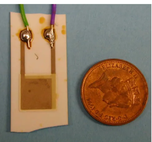
In addition, it has been decided to produce two versions of the transducers: one with the so-called guard electrode and the second without, which coupled together in a single ‘measurement cell’, would reduce fringe effects of electrical field used for electrical measurements (similarly as discussed, for example, in [16]). All these considerations, which are not covered in detail here, lead to the final design which is described in the following sections. A photograph of one of the early sensors (with the active area of 10 ×10 mm2_{) is}

shown in figure2.

The suitability of materials for application in the dual-modality sensors under development was tested through their exposure to saline water at the pressure of 150 bar and the temperature of 150◦C. A single immersion test, carried out in a purpose-built autoclave located in the School of Mechanical and Systems Engineering, University of Newcastle, would normally last about a week. The sensor evaluation would typically include visual inspection for signs of corrosion on metal electrodes and comparison between measurement

Figure 2.One of the early thick-film sensors with active area of 10×10 mm2_.

performance ‘before’ and ‘after’ the immersion. The main outcomes from these studies were application of gold for the electrode material—sensors using less expensive silver– palladium showed serious corrosion problems, and use of PZT powder 5A—one of the few piezoceramic materials that did not show deterioration of measurement performance in ultrasonic measurement mode.

3.2. Sensor fabrication process

The fabrication of transducers was undertaken at the University of Southampton within the School of Electronics and Computer Science. The devices were made using thick-film technology, with which the Southampton group have considerable experience [1]. The overall structure of the two versions of sensors is shown schematically in figure3.

With reference to figure 3, the substrate material was 96% alumina of thickness 635µm. Each electrode layer was fabricated with a gold thick-film paste and the piezoelectric layer was a purpose formulated paste developed at the University of Southampton. Lead zirconate titanate (PZT) powder type 5A, manufactured by Morgan Electroceramics Ltd, was chosen as the active material for the piezoelectric paste. This has a Curie temperature in the region of 350◦C, allowing the sensors to operate at the desired specification of 150◦C. The size of the lower gold electrode is 10×10 mm2

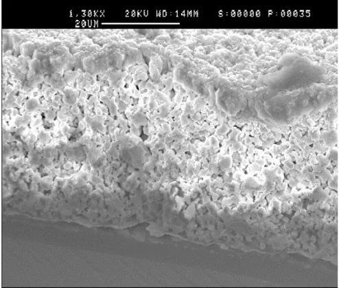
and this is screen printed onto the alumina substrate, dried in an infra-red drier at about 150◦C and then fired in a belt furnace at a peak temperature of 890◦C. The thick-film PZT layer of size just sufficient to overlap the bottom electrode was printed twice in order to obtain a thickness of around 50µm and then subjected to a similar firing profile to the initial layer. Figure4shows a microscopic view of the PZT layer deposited on the substrate.

(a) (b)

Figure 3.Schematic of the layer configuration in the thick-film sensor: (a) version with the ring guard electrode; (b) version with plane electrode.

Figure 4.Microscope view of deposited PZT material.

layer is a square with dimensions 20×20 mm2_{. The resulting}

devices are essentially planar capacitor-type structures. After processing, the PZT layer has to be polarized in order to induce piezoelectric behaviour. This is achieved by placing the substrate on a hot plate at a temperature of around 120◦C and applying a dc electric field of 4 MV m−1across the sample for 10 min.

Figure 5 shows a photograph of the two types of transducers fabricated, together with the photograph of a sensor assembly in the form of a test cell, used in laboratory experiments.

3.3. Test cell set-up

Although the ultimate objective of the work described in this paper is the development of a dual-modality sensor, capable of both the ultrasonic and electrical measurements, at the current stage such measurements were not performed simultaneously. This is simply a matter of practicalities of the measurement equipment. The ultrasonic pulser–receiver system generates voltage bursts (spikes) of the amplitude of 400 V, and when such measurements are conducted, the LCR meter for electrical measurements must be disconnected to

avoid possible damage. In future, an electronic circuit to isolate the two systems must be developed, but it was not felt important at this stage.

As shown in figure 5, the sensors had short lengths of cables soldered at the edge. These would then be connected to the miniature co-axial cables (RG174 type) which were fed to either the pulser–receiver system or the LCR meter. When using the pulser–receiver system, ports A and B on one side of the cell and ports D and E on the other side would be used. In this way, the PZT wafer could be excited to generate the pressure wave on one of the sensors, which could then be detected on the other sensor using time-of-flight measurement principle. When using the LCR meter, the excitation voltage, carried via the core of a coaxial cable, would be connected to port E, while the shield of that cable would be connected to a copper plate on the outside of the cell (which can be seen in figure 5(c)). On the other side of the cell, the detected signal, carried in the core of the second coaxial cable, would be taken from port B. The shield of the second cable would be connected to port C (the ring guard electrode) and the external shield, ‘behind’ the cell shown in figure5(c).

1

2

3

4

5

A _C

B

D E

(a) (b) (c)

1

2

3

4

5

A _C

B

D E

(a) (b) (c)

Figure 5.Photograph of the thick-film sensors: (a) with ring guard electrode, (b) plane, (c) sensor assembly in the form of a ‘test cell’.

LCR Meter

Pulser-receiver

Thermostatic bath

Data acquizition

1 2

3

1 – test cell 2 – thermometer

3 – high shear homogenizer

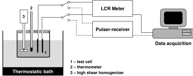
Figure 6.Schematic of the experimental arrangement.

of the ultrasonic measurements unacceptable. Large spacing, on the other hand tends to reduce the guarding effect of the ring electrode. The preliminary studies showed that an acceptable distance between the sensors used here is in the range of 12–20 mm.

4. Experimental set-up

The experimental set-up used in the measurements described here is shown schematically in figure6. The heterogeneous mixtures investigated were contained in a 500 ml glass beaker, which was immersed in a thermostatic bath of preset temperature. The measurements, taken by either the LCR meter or the pulser–receiver, were stored on a data acquisition PC.

4.1. Preparation of fluids

For reasons of safety and practical issues concerned with using clean and inexpensive media, the fluids normally present in oil and gas extraction (crude oil and formation water) were simulated by the use of vegetable oil and distilled water with 200 g of sodium chloride added per litre (20% by weight). The high content of sodium chloride in water was chosen to mimic the density of the formation water present in oil extraction processes, which can often reach levels of 1.1–1.2 g cm−3_.

Future experiments are planned, which will use more realistic fluids.

In order to obtain stable mixtures (emulsions), an aqueous surfactant solution was prepared by dissolving 1% by weight of Tween-20 (ICI Chemicals & Polymers Ltd) in saline water (1% measured relative to the original distilled water). The

vegetable oil-in-saline water emulsion was prepared by mixing vegetable oil with saline water in a glass beaker and blending it with a homogenizer (IKA Ultra-Turrax T25) at a rotational speed of 22 000 rpm. A series of oil-in-saline water emulsions with volume concentrations of oil varying between 0% and 50% with steps of 10% was prepared. Similarly, a series of saline water-in-oil emulsions with volume concentrations of water between 0% and 50% in steps of 10% was prepared using a similar procedure. In the latter case, to avoid confusion, instead of measuring water contents in oil, the mixtures are identified by oil volume fraction which varies between 50% and 100%.

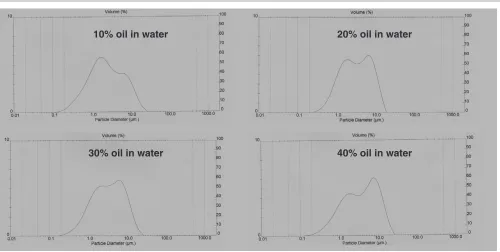
The obtained emulsions were stable for periods ranging from a few hours to a few days. This allowed bringing the sample fluids to the desired temperature within the thermostatic bath, while measurements on other samples were being conducted. When signs of separation were appearing, the mixtures could also be easily re-mixed for a few minutes, while waiting for their turn of the measurements. To ensure comparable results, the distribution of droplet size was occasionally measured using a particle size analyser (Mastersizer by Malvern Instruments Ltd). A set of typical droplet size distributions is shown in figure7. The horizontal axis is a logarithmic scale showing particle diameters, while the vertical axis corresponds to the probability density distribution. As can be seen, the droplet sizes were typically in the range of 1.0–10.0 µm. It is interesting to note that the distributions look as though consisting of two separated distributions (double peaks), which is likely to have been caused by the aforementioned occasional re-mixing of mixtures.

10% oil in water 20% oil in water

40% oil in water 30% oil in water

Figure 7.Droplet size distribution measured by Malvern Mastersizer for a few selected oil-in-water concentrations.

Figure 8.An example of time history of send and received signals (arbitrary scales).

thermostatic bath (Clifton model 49700), and measured independently using a mercury thermometer inserted directly into the sample, with an accuracy of 0.5◦. The investigations were limited to four selected temperatures: 25, 30, 40 and 50◦C.

4.2. Electrical and ultrasonic measurement systems

The ultrasonic transmission measurements were made using the ultrasonic flaw detector (model EPOCH II, 2100 series, manufactured by Panametrics Ltd). The band widths of the detector are selectable from a lower limit (5 or 500 kHz) to an upper limit (2.25, 6 or 15 MHz). The energy levels can be selected as 8, 32 or 128µJ. In the first approximation, the accuracy of the time-of-flight measurements can be estimated from the ability of the device to resolve the time history of the pulse send from the excitation transducer and the pulse received on the detector, which for this particular model is ±0.0125 µs. This alone gives about ±2 m s−1 error of velocity measurements based on 20 mm gap between the sensors and a typical velocity in the range of 1500– 1800 m s−1for the investigated fluids. The time-of-flight is measured from the distance between the send and the received signals, from the graphs such as the one shown in figure 8

1350 1400 1450 1500 1550 1600 1650 1700 1750

20 25 30 35 40 45 50 55

Temperature [oC]

Speed of Sound [m

/s] _{saline water}

distilled water vegetable oil

Figure 9.Speed of sound measured by the thick-film sensor in pure liquids as a function of temperature.

(knowing the horizontal time scale displayed on the computer screen). Therefore, in addition to the errors related to the temporal resolution, an error of the ‘subjective judgement’ of the researcher as to when the pressure wave arrives at the receiver must be considered. This most likely gives rise to a ‘systematic’ error as will be discussed later.

1350 1400 1450 1500 1550 1600 1650 1700 1750

0 10 20 30 40 50 60 70 80 90 100

Oil concentration [%]

Speed of Sound [m

/s]

25 deg C 30 deg C 40 deg C 50 deg C

Figure 10.Speed of sound in emulsions at different oil concentration and at different temperatures.

and connected to the second electrode. In the experiments described in this paper, the excitation level used was 1 V and the electrical properties were measured at three selected frequencies: 10 kHz, 100 kHz and 1 MHz.

5. Sample experimental results and discussion

5.1. Ultrasonic measurement

The initial measurements were conducted to gain some confidence in the data acquired from thick-film sensors. The

(a)

(c)

(b)

(d )

0.58 0.6 0.62 0.64 0.66 0.68 0.7 0.72 0.74

0 10 20 30 40 50 60 70 80 90 100

Oil concentration [%]

0 10 20 30 40 50 60 70 80 90 100

Oil concentration [%]

0 10 20 30 40 50 60 70 80 90 100

Oil concentration [%]

0 10 20 30 40 50 60 70 80 90 100

Oil concentration [%]

1000/(speed of sound)

[s

/m]

0.58 0.6 0.62 0.64 0.66 0.68 0.7 0.72 0.74

1000/(speed of sound)

[s

/m]

0.58 0.6 0.62 0.64 0.66 0.68 0.7 0.72 0.74

1000/(speed of sound)

[s

/m]

0.58 0.6 0.62 0.64 0.66 0.68 0.7 0.72 0.74

1000/(speed of sound)

[s

/m]

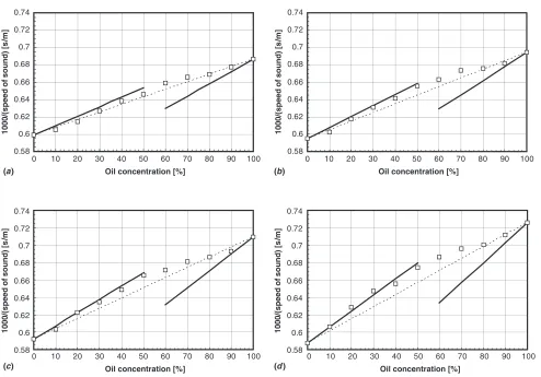
Figure 11.Comparison of the experimental results (open squares) with the theoretical predictions by Tavlarides and co-workers (solid line corresponds to equation (17), dashed line to time-average model (16). The graphs (a)–(d) correspond to temperatures 25, 30, 40 and 50◦C, respectively.

speed of sound for pure liquids, distilled water, saline water and vegetable oil, at different temperatures, was measured. Figure9summarizes the data obtained. It is worth pointing out that the obtained speed of sound for distilled water at 25◦C was 1491 m s−1, while the existing literature gives a value of 1496.7 m s−1[32] or 1497 m s−1[38]. Interestingly, the speed of sound in distilled water for 50 ◦C has been measured as 1531 m s−1_{against the literature value of 1541 m s}−1_{. This}

suggests that the curve for distilled water is in the actual fact shifted by about 7–8 m s−1downwards (compared to literature data), which suggests a ‘systematic’ error mentioned in section4.2. It is reasonable to assume that similar errors are present in the data for saline water and vegetable oil. However, no attempt was made to correct the data at this stage as the discrepancies discussed here have little consequence for the ability of the sensor to measure the mixture composition based on the ultrasonic transmission time.

Figure9 shows that the speed of sound in both distilled and saline water increases with the increase of the temperature, while the speed of sound in vegetable oil decreases with the increase of the temperature. This is in agreement with existing literature [39].

0.1 1 10 100 1000 10000

0 10 20 30 40 50 60 70 80 90 100

Oil concentration [%] Oil concentration [%]

0 10 20 30 40 50 60 70 80 90 100

Oil concentration [%] Oil concentration [%]

0 10 20 30 40 50 60 70 80 90 100

Oil concentration [%] Oil concentration [%]

0 10 20 30 40 50 60 70 80 90 100

Oil concentration [%] Oil concentration [%]

Capacitance [pF]

0.1 1 10 100 1000 10000

Capacitance [pF]

0.1 1 10 100 1000 10000

Capacitance [pF]

0.1 1 10 100 1000 10000

Capacitance [pF]

f = 10 kHz

f = 100 kHz

f = 1 MHz

0.001 0.01 0.1 1 10 100 1000 10000 100000

0 10 20 30 40 50 60 70 80 90 100

Conductance [

µ

S]

Conductance [

µ

S]

Conductance [

µ

S]

Conductance [

µ

S]

f = 10 kHz

f = 100 kHz

f = 1 MHz

f = 10 kHz

f = 100 kHz f = 1 MHz

0.001 0.01 0.1 1 10 100 1000 10000 100000

0 10 20 30 40 50 60 70 80 90 100

f = 10 kHz

f = 100 kHz f = 1 MHz

f = 10 kHz f = 100 kHz

f = 1 MHz

0.001 0.01 0.1 1 10 100 1000 10000 100000

0 10 20 30 40 50 60 70 80 90 100

f = 10 kHz f = 100 kHz

f = 1 MHz

f = 10 kHz f = 100 kHz

f = 1 MHz

0.001 0.01 0.1 1 10 100 1000 10000 100000

0 10 20 30 40 50 60 70 80 90 100

f = 10 kHz f = 100 kHz

f = 1 MHz (a)

(b)

(c)

(d)

(e)

(f)

(g)

(h)

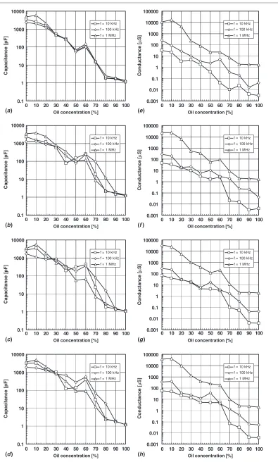
Figure 12.Results of electrical measurements using thick-film transducer: (a)–(d) electrical capacitance for 25, 30, 40 and 50◦C, respectively; (e)–(h) electrical conductance for 25, 30, 40 and 50◦C, respectively.

The experimental data obtained during the investigation were compared with the theoretical model developed by

(a) 0.001

0.01 0.1 1 10 100 1000

0 10 20 30 40 50 60 70 80 90 100

Oil concentration[%]

(b) 0 10 20 30 _{Oil concentration[%]}40 50 60 70 80 90 100

Normalized capacitance (water side)

0.001 0.01 0.1 1 10 100 1000

Normalized capacitance (water side)

0.001 0.01 0.1 1 10 100 1000

f = 10 kHz f = 100 kHz f = 1 MHz Theory f = 10 kHz f = 100 kHz f = 1 MHz Theory

0.001 0.01 0.1 1 10 100 1000

Normalized conductance (oil side)

Normalized conductance (oil side)

f = 10 kHz f = 100 kHz f = 1 MHz Theory f = 10 kHz f = 100 kHz f = 1 MHz Theory

Figure 13.Comparison between electrical properties measured by the thick-film sensor and the theoretical model developed by Hammer

et al[13].

when the inverse of the speed of soundv∗is plotted against the volumetric concentrationφas follows:

1

v∗ =φ

gd,i

vd

−gc,i

vc

+ 1

vc .

Using the coefficient γ defined by equation (18) and calculating coefficientsgd,iandgc,idefined by equations (19) and (20), as appropriate, the theoretical prediction can be visualized on the same graph as the experimental data. This comparison is shown in figure 11for the four temperatures considered. Here the experimental points are shown as open squares, while the solid lines correspond to the theoretical prediction. It is clear that the theory and the experimental results agree very well for water continuous mixtures (left-hand side of the graphs), while there is very little agreement for oil continuous mixtures (water phase dispersed). It is difficult to speculate as to the reasons for such a discrepancy; however, it should be noted that the variation in density between the media used here is much wider than that considered in [34]. Judging from the graphs in figure11, the time-average model (see the thin dashed lines) given by equation (16) could be more

suitable for emulsions with dispersed water than equation (17) with complicated coefficients (20).

5.2. Electrical measurement

oil concentration—i.e. high conductance for water phase, low conductance for oil phase and an almost monotonic decrease between the two extremes—it seems that the conductance measurements obtained using the measurement system available would be more difficult to interpret in terms of oil concentration, because of the lack of consistency, perhaps best exemplified by the curves obtained forf =10 kHz and

f=100 kHz at the oil-continuous end of the graph.

Some comparisons with a simple model given in [13] were attempted. The measured capacitance and conductance values were firstly normalized by dividing them by the capacitance or conductance values obtained for pure media (for each of the frequencies). In this way, the curves would always start from the value of 1 and rise (or drop) depending on whether the curve is drawn from the ‘water side’ (i.e. to the right) or from the ‘oil side’ (i.e. to the left). If the theory outlined by Hammeret al[13] was applicable to the mixtures investigated here, the experimental data for the water-continuous mixtures should collapse onto the line 2β/(3−β), while the data for the oil-continuous mixtures should collapse onto line (1 + 2β)/

(1−β), where β is the water cut (easily calculated from oil concentration as the difference between 100% and the oil concentration and expressed as a decimal value between 0 and 1). The result of such procedure for the temperature of 25 ◦C is in fact shown in figure13; however, it can be easily recognized that only partial agreement can be found for capacitance measurements for oil concentrations between 0% and 20% (water continuous mixtures) and oil concentrations between 80% and 100% (oil continuous mixtures).

It is not clear as to why a better agreement between the measurements and the theoretical predictions cannot be found. However, the measurements in highly conductive media are notoriously difficult and perhaps the LCR meter used (designed primarily for testing electronic components) is not adequate for high-accuracy measurements in heterogeneous mixtures. Secondly, for simplicity, a two-terminal measurement arrangement was used; a four-terminal method could potentially offer higher quality. Finally, the model proposed by Hammeret al [13] is only one of the simplest available. It may be necessary to consider more complex models in any future work, such as given in equations (7) and (8). Nevertheless, from the sensor design point of view, the important issue is the ability of the sensors to provide information on the electrical properties of heterogeneous mixtures, which could be usefully utilized in future industrial applications.

6. Conclusion

A novel multi-modal sensor for measurement of the composition of heterogeneous mixtures has been developed. The sensor design utilizes the thick-film fabrication technology, which enables incorporation of the electrical measurement modality and ultrasonic time-of-flight measurement in a single device. The sensor was developed with the needs of oil and gas extraction industry in mind where high pressure, high temperature and aggressive media are a common occurrence. These requirements have been addressed by using the ceramic substrate and high-quality sensor material such as golden electrodes and specially

formulated PZT pastes for the ultrasonic transducer. How-ever, it is hoped that the sensors developed could be used in other areas including chemicals, biotechnology, pharma-ceutical or food and drink, which may be operationally less demanding.

The rationale behind developing such a dual-modality sensor has been outlined and the preliminary studies, design activities and the fabrication process have been summarized. The sensor developed was subjected to environmental testing at high- pressures and temperatures as well as a series of laboratory experiments aiming to evaluate its ability to provide useful information about the characteristics of heterogeneous mixtures. These procedures have been presented, together with selected experimental data. The experimental results have been analysed and compared with simple models governing the behaviour of heterogeneous mixtures. It is concluded here that the dual-modality sensors developed can be usefully utilized for the characterization of the heterogeneous mixtures. It is probably useful to point out that in any practical implementation, there will be a need for providing temperature measurements, as any characteristics of heterogeneous mixtures will be temperature dependent. This can be easily achieved by using a standard thermocouple, or alternatively a way of depositing a thick-film based thermocouple could be incorporated into the sensor manufacturing process.

Clearly, the work presented here was of preliminary character. Several areas of future development can be identified. Firstly, the design of the sensors will inevitably evolve and will need to be refined. At this stage, it is thought that the following additional work may be required: (i) provision of suitable coatings on the sensor surface, such as glassy materials, (ii) cyclic temperature testing of the sensor to ascertain the potential problems caused by factors such as permeation of humidity, loss of integrity of the outer metallization layer or mismatch of thermal expansion in various layers used: alumina, gold, PZT and any external coating, (iii) optimization of the sensors from the point of view of the conversion of the electrical energy fed to ultrasonic sensor into the mechanical energy of the pressure wave is needed.

Secondly, a better understanding of the electrical and acoustic characteristics of realistic mixtures, obtained using the thick-film sensors, is required. This needs to include broader studies of the practical industrial fluids, including, for example, a range of mixtures of crude oil and formation water or a variety of emulsions found in the food and drink industry, as well as utilization of use of more accurate impedance analysers as well as simulation of the sensor performance using electrical and acoustic field solvers. One interesting question would be whether it is possible to push the electrical measurement range towards microwave frequencies.

Acknowledgments

The authors would like to gratefully acknowledge the support from EPSRC under the grant number GR/R35858. Guangtian Meng would like to acknowledge the support obtained from Oilfield Technology Limited and Universities UK for his postgraduate studies at the University of Manchester.

References

[1] White N M and Turner D 1997 Thick-film sensors: past, present and futureMeas. Sci. Technol.81–20 [2] Kress-Rogers E and Brimelow C J B (ed) 2001

Instrumentation and Sensors for the Food Industry2nd edn

(Cambridge: CRC Press/Woodhead Publishing Limited) [3] Baxter L K 1996Capacitive Sensors: Design and

Applications(New York: IEEE)

[4] van Beek L K H 1967 Dielectric behaviour of heterogeneous systemsProg. Dielectr.769–114

[5] Hanai T 1968Electrical properties of emulsions Emulsion

Scienceed Sherman P (London and New York: Academic)

chapter 5

[6] Maxwell J C 1873A Treatise on Electricity and Magnetism vol I (Oxford: Clarendon)

[7] Rayleigh J W S B 1892 On the influence of obstacles in rectangular order upon the properties of a mediumPhil.

Mag.34481

[8] Wiener O 1912 Die theorie des mschkorpers f¨ur dir feld der stationaren stromungAbh. d. Sach. Ges. d. Wiss.,

Math.-Phys. K132509

[9] B¨ottcher C J F 1952Theory of Electric Polarisation (New York: Elsevier)

[10] Wagner K W 1914Arch. Elektrotech.2371 [11] Rao N Y and Ramu T S 1972Determinationof the Q1

permittivity and loss factor of mixtures of liquid dielectrics

IEEE Trans. Electric. Insul.E1-7

[12] Ramu T S and Rao N Y 1973Onthe evaluation of Q2

conductivity of mixtures of liquid dielectricsIEEE Trans.

Electric. Insul.8

[13] Hammer E A, Tollefsen J and Cimpan E 1997 The importance in calculating the permittivity and conductivity in two component mixtures for image reconstructionProc. Engineering Foundation Conference: Frontiers in

Industrial Process Tomography II (April 9–12)(The

Netherlands: Delft University of Technology) pp 235–40 [14] Strizzolo C N and Converti J 1993 Capacitance sensors for

measurements of phase volume fraction in two-phase pipelinesIEEE Trans. Instrum. Meas.42726–9 [15] Beck M S, Green R G, Hammer E A and Thorn R 1985

On-line measurement of oil/gas/water mixtures, using a capacitance sensorMeasurement37–14

[16] Jaworski A J, Dyakowski T and Davies G A 1999 A capacitance probe for interface detection in oil and gas extraction plantMeas. Sci. Technol.10L15–20

[17] Davies G A, Dyakowski T and Jaworski A J 2002 Sensor array for detecting electrical characteristics of fluidsUS Patent 6,419,807, July 16, 2002

[18] Engebretsen B and Halleraker J M 2002 Apparatus for capacitive electrical detectionUS Patent Application US/2002/0070734

[19] Santa Maria A F, Banerjee P K and Vincent J F Jr 1997 Capacitive oil water emulsion sensor systemUS Patent 5,642,098, June 24, 1997

[20] Schr¨oder J, Doerner S, Schneider T and Hauptmann P 2004 Analogue and digital sensor interfaces for impedance spectroscopyMeas. Sci. Technol.151271–8

[21] Povey M J W and McClements D J 1988 Ultrasonics in food engineering. Part I: introduction and experimental methods

J. Food Eng.8217–45

[22] McClements D J and Povey M J W 1987 Ultrasonic velocity as a probe of emulsions and suspensionsAdv. Colloid

Interface Sci.27285–316

[23] Povey M J W 1989 Ultrasonics in food engineering. Part II: ApplicationsJ. Food Eng.91–20

[24] Povey M J W 1998 Ultrasonics in foodContemp. Phys.39

467–78

[25] McClements D J and Povey M J W 1989 Scattering of ultrasound by emulsionsJ. Phys. D: Appl. Phys.22

38–47

[26] McClements D J, Povey M J W, Jury M and Betsanis E 1990 Ultrasonic characterisation of a food emulsionUltrasonics 28266–72

[27] Pinfield V J, Povwy M J W and Dickinson E 1995 The application of modified forms of the Urick equation to the interpretation of ultrasound velocity in scattering systems

Ultrasonics33243–51

[28] Pinfield V J and Povey M J W 1997 Thermal scattering must be accounted for in the determination of adiabatic compressibilityJ. Phys. Chem.B1011110–2 [29] Tong J and Povey M J W 2002 Poulse echo comparison

method with FSUPER to measure velocity dispersion in n-tetradecane in water emulsionsUltrasonics40

37–41

[30] Urick R J 1947 A sound velocity method for determining the compressibility of finely divided substancesJ. Appl. Phys. 18983–7

[31] Wood A B 1941A Textbook of Sound(London UK: Bell and Sons)

[32] Bonnet J C and Tavlarides L L 1987 Ultrasonic technique for dispersed-phase holdup measurementsInd. Eng. Chem. Res. 26811–15

[33] Yi J and Tavlarides L L 1990 Model for hold-up measurements in liquid dispersions using an ultrasonic techniqueInd. Eng.

Chem. Res.29475–82

[34] Tsouris C and Tavlarides L L 1990 Comments on Model for hold-up measurements in liquid dispersions using an ultrasonic techniqueInd. Eng. Chem. Res.292170–2 [35] Tsouris C, Tavlarides L L and Bonnet J C 1990 Application of

the ultrasonic technique for real-time holdup monitoring for the control of extraction columnsChem. Eng. Sci.45

3055–62

[36] Tsouris C and Tavlarides L L 1991 Control of dispersed-phase volume fraction in multistage extraction columnsChem.

Eng. Sci.462857–65

[37] Dyakowski T, Hale J M, Jaworski A J and White N M 2004 A sensing devicePatent ApplicationPCT/GB2004/003805 [38] Schulitz F T, Lu Y and Wadley H N G 1998 Ultrasonic

propagation in metal powder-viscous liquid suspensions

J. Acoust. Soc. Am.1031361–9

[39] Koˇciš Š and Figura Z 1996Ultrasonic Measurements and

Technologies (Sensor Physics and Technologyvol 4)

Queries

(1) Author: Please provide page range for this references [12] and [13].