Split domain calibration of an ecosystem model using satellite ocean colour data

Split-domain calibration of an ecosystem

model using satellite ocean colour data

John C. P. Hemmings

∗

, Meric A. Srokosz, Peter Challenor,

Michael J. R. Fasham

Southampton Oceanography Centre, European Way, Southampton SO14 3ZH, UK

Abstract

The application of satellite ocean colour data to the calibration of plankton ecosys-tem models for large geographic domains, over which their ideal parameters cannot be assumed to be invariant, is investigated. A method is presented for seeking the number and geographic scope of parameter sets which allows the best fit to vali-dation data to be achieved. These are independent data not used in the parameter estimation process. The goodness-of-fit of the optimally calibrated model to the validation data is an objective measure of merit for the model, together with its ex-ternal forcing data. Importantly, this is a statistic which can be used for comparative evaluation of different models. The method makes use of observations from multiple locations, referred to as stations, distributed across the geographic domain. It relies on a technique for finding groups of stations which can be aggregated for parameter estimation purposes with minimal increase in the resulting misfit between model and observations.

The results of testing this split-domain calibration method for a simple zero-dimensional model, using observations from 30 stations in the North Atlantic, are presented. The stations are divided into separate calibration and validation sets. One year of ocean colour data from each station were used in conjunction with a climatological estimate of the station’s annual nitrate maximum. The results demon-strate the practical utility of the method and imply that an optimal fit of the model to the validation data would be given by two parameter sets. The corresponding division of the North Atlantic domain into two provinces allows a misfit-based cost to be achieved which is 25% lower than that for the single parameter set obtained using all of the calibration stations. In general, parameters are poorly constrained, contributing to a high degree of uncertainty in model output for unobserved vari-ables. This suggests that limited progress towards a definitive model calibration can be made without including other types of observations.

Key words:

1 Introduction

An ability to predict the response of the pelagic ecosystem to physical changes in the environment is a prerequisite for quantifying potentially important cli-mate feedbacks involving the marine carbon cycle. Progress in this area re-quires the development of ecosystem models which can be used to extrapolate reliable biological predictions from external forcing data describing physical variability. These models can be coupled with basin-scale or global-scale gen-eral circulation models. Useful preliminary results have already been obtained in this way with some specific ecosystem models (e.g. Sarmiento et al., 1993; Oschlies and Gar¸con, 1998; Oschlies et al., 2000; Sarmiento et al., 2000; Gregg, 2001; Oschlies, 2001; Palmer and Totterdell, 2001; Christian et al., 2002). However, a wide range of candidate ecosystem models are available, varying in complexity and employing many different structures and functional forms. Evaluating their relative merits in an objective way poses a major challenge.

All of the candidate models contain a large number of parameters, many of which are poorly known or represent quantities which, in nature, are highly variable in time and space and across taxa. Parameter uncertainty acts as a barrier to the evaluation of one model against another. The models need first to be calibrated against observational data. This has been done for a number of models using time series data collected at various sites. The Bermuda Atlantic Time-series Study (BATS 32◦_{N 64}◦_{W) site has received particular attention}

(Hurtt and Armstrong, 1996, 1999; Spitz et al., 1998; Fennel et al., 2001; Spitz et al., 2001; Schartau et al., 2001). Calibrations have also been performed for Ocean Weather Station Papa (50◦_{N 145}◦_{W) in the Pacific (Matear, 1995;}

Prunet et al., 1996a,b), the North Atlantic Bloom Experiment site at 47◦_N,

20◦_{W (Fasham and Evans, 1995; Evans, 1999) and at the Tropical Atmosphere}

Ocean mooring at 140◦_{W in the equatorial Pacific (Friedrichs, 2002). Hurtt}

and Armstrong (1999) calibrated a model using BATS data and observations from Ocean Weather Station India (OWSI 59◦_{N 20}◦_{W) simultaneously. These}

studies are all based on in situ data although satellite ocean colour measure-ments, now routinely available from SeaWiFS (McClain et al., 1998) and other sensors, are now beginning to be used to improve the coverage of the annual cycle (Friedrichs, 2002).

Model parameters are estimated by first defining either a cost function or a likelihood function, based on the misfit between the model output and obser-vations. This is a function of the model’s parameter set, defined by a vector in the model’s parameter space. An optimization technique is then applied to search the parameter space for values which minimize the cost or maximize

∗ _{Corresponding author. Fax: +44 (0)23 8059 6400}

the likelihood. In a number of cases the calibration studies are supported by identical twin experiments in which simulated observations, sometimes includ-ing stochastic errors, are assimilated in an attempt to recover the parameter set of the model from which they were generated (Spitz et al., 1998; Fennel et al., 2001; Spitz et al., 2001; Schartau et al., 2001; Friedrichs, 2001). These experiments provide important information on the robustness of the optimiza-tion methods and the ability of different numbers and types of observaoptimiza-tions to constrain parameter values independently, under the assumption that the model is a perfect description of reality. However, as pointed out by Schar-tau et al. (2001) inferences from twin experiments are only strictly applicable to optimization results for real observations if the reference parameter values used to generate the simulated observations are close to the optimum values sought for describing the real data.

While an important goal in climate modelling is to develop models which can be applied globally, virtually all of the calibrations performed so far are based on observations at single locations. The geographic scope over which they can be usefully applied has yet to be properly assessed, although Hurtt and Armstrong (1999) did examine the performance of their model, calibrated using Atlantic observations, at the Hawaii Ocean Time-series site in the Pa-cific. Formal validation of model output against independent data not used in the parameter estimation process, whether this be local data for a different time period or data from another location, is important for quantifying the predictive skill of a model. The calibrated models of Prunet et al. (1996a,b) and Friedrichs (2002) were tested against independent local data. However, in general, this aspect of model evaluation has so far received relatively little attention. Satellite ocean colour measurements provide estimates of surface chlorophyll concentration over multiple annual cycles throughout most of the world ocean. They are therefore an invaluable resource for calibrating and val-idating models and for analysing the geographic scope of models which have been calibrated for specific locations.

Although ocean colour measurements give information relating to phytoplank-ton components of the ecosystem only, their use in model calibration in con-junction with other observations should lead to more widely applicable param-eter vectors. The exploitation of these data for such purposes is just beginning. Losa et al. (submitted) have recently used ocean colour data to examine the variability in model parameters arising from local calibrations over the North Atlantic basin, while Hemmings et al. (2003) attempted to retrieve parameter vectors applicable over a wide range of different environmental conditions by fitting a model simultaneously at multiple stations. The present study builds on the latter work, seeking the most effective way of using ocean colour data in model calibration and validation.

it is implicitly assumed that the same parameter vector is appropriate for all locations and that spatial variability is purely a result of the different environ-mental conditions described by the model’s external forcing data. However, as demonstrated for the North Atlantic (Hemmings et al., 2003), assuming a

priori that a single parameter vector is appropriate for a large domain can

lead to a sub-optimal calibration. Differences may exist between ecosystems in different regions which are independent of factors represented in the forc-ing data, but can be reproduced by different parameter vectors. The most obvious example is differences in the taxonomic composition of the plankton. It is therefore desirable to investigate whether better results can be obtained by splitting the geographic domain into provinces and calibrating the model separately for each. This immediately introduces the problem of how best to split the domain. One possible approach is to use the biogeochemical provinces defined by Longhurst (1998), which are based on observed spatial variation in the characteristics of the annual phytoplankton cycle, combined with our knowledge of the relevant physical features of ocean regions. However, the extent to which the observed differences in the annual cycle imply significant differences in the ecosystem response to physical forcing, as opposed to simply reflecting the variability in that forcing, is unclear. We present here a more flexible approach, which does not require any prior assumptions about the geographic scope of individual parameter vectors. The utility of the method is tested by applying it to a simple candidate model.

A major problem in model calibration is the difficulty of locating the global minimum of a cost function in parameter space. The effects of different pa-rameters on model output are often correlated, potentially making the inverse problem underdetermined, even in identical twin experiments where the model is perfect and there is no observational error. In real applications, model inad-equacy, observation error and poor data availability compound the problem. Observational constraints on parameter values are normally weak and the existence of a single global minimum which is significant in the presence of observational error is unlikely. Fortunately though, to objectively choose be-tween models we do not actually need to locate the cost function minimum for each in the parameter space, provided we can estimate its value. There-fore, in contrast with previous work, the emphasis here is on estimating the minimum cost obtainable for the given model, together with the associated posterior parameter probability distribution(s), rather than on finding a single optimal parameter vector for each province. While it is unnecessary for the parameters to be independently constrained by the observations to estimate the minimum cost, the extent to which they can be constrained does have important implications for the uncertainty associated with model predictions. The uncertainty in model output associated with the posterior parameter dis-tributions is therefore examined.

then describes how the method was tested by using it to evaluate the candidate model for the North Atlantic. The results of the test are presented in Section 4 and the utility of the method is discussed in Section 5.

2 The calibration method

2.1 Overview

The calibration procedure involves minimizing a cost based on the misfit be-tween model output and observations at multiple locations in the model do-main, referred to as stations. These stations are divided into two sets. One is a calibration set, from which stations are combined in different calibration groups to obtain parameter vector estimates. The other is a validation set. Data from these stations are not used in the parameter estimation process. Instead they are used to evaluate alternative model calibrations, each specified either by one parameter vector for the whole domain or a number of provin-cial parameter vectors which together cover the domain. These independent validation data are vital for assessing the generality of the calibrated model and thereby its value for prediction.

The division of stations between the calibration and validation sets is done in such a way that the data in each set are statistically similar, constituting independent samples from the same population. In order that calibrations in-volving multiple parameter vectors can be tested, it is important that each set provides similar coverage of any given geographic region. We expect similar results whichever set is chosen as the calibration set. This assumed robust-ness to sampling error is supported by the results of Hemmings et al. (2003). They showed that compatible parameter estimates could be obtained by fit-ting a model to 3 independent basin-wide calibration sets, provided each set was similarly distributed over the range of different environmental conditions present.

The algorithm for finding the optimal calibration is to first seek the best single-parameter vector calibration for the domain and then investigate whether a better calibration can be obtained by splitting the domain into two geographic provinces. If one or more ways of splitting the domain are found which lead to improved calibrations, then the best domain division is accepted and the algo-rithm is recursively applied to each province until either there is no decrease in the validation cost or no practical geographic split is possible.

It is not assumed that the best single-parameter vector calibration for a do-main is the one that uses all the calibration stations. There may be good reason to exclude atypical stations to prevent them adversely affecting the calibration result. Such atypical stations might exist due to real but local ef-fects, poor forcing data or differences in the type or number of observations available. Instead a novel method of aggregating stations into ‘natural’ cali-bration groups is employed. This allows groups comprising different numbers of stations to be identified, each of which is the group of a particular size best satisfied by a single parameter vector. No account is taken of the station posi-tions prior to aggregation, but the geographic distribution of staposi-tions in each of the emerging groups is examined. Large groups with good coverage of the domain provide alternative calibration groups for the undivided domain. In addition, any of the smaller groups in which stations are geographically clus-tered indicates a natural province within the domain, on the basis of which a trial split-domain calibration can be performed.

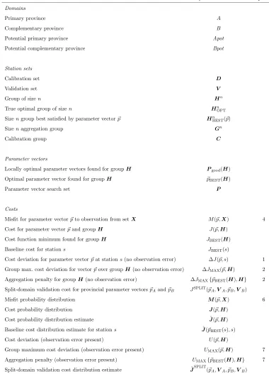
The calibration algorithm is implemented by a hierarchy of procedures which are described in the following sub-sections, starting from the lowest level. The most fundamental of these, the ‘parameter optimization procedure’ is invoked by the ‘station aggregation procedure’ which is in turn invoked by two higher-level procedures to identify optimal provinces and calibration groups. Finally Section 2.5 describes important modifications to the basic method which allow observation error to be taken into account. For reference, a list of standard terms and symbols used in the description is given in Table 1.

2.2 Parameter optimization

be-Table 1

Standard notation for the split-domain calibration method

Item Symbol or function Equation

Domains

Primary province A

Complementary province B

Potential primary province Apot

Potential complementary province Bpot

Station sets

Calibration set D

Validation set V

Group of sizen Hn

True optimal group of sizen Hn_OPT

Sizengroup best satisfied by parameter vector~p Hn

BEST(~p)

Sizenaggregation group Gn

Calibration group C

Parameter vectors

Locally optimal parameter vectors found for groupH P_good(H₎

Optimal parameter vector found for groupH _~pBEST(H₎

Parameter vector search set P

Costs

Misfit for parameter vector~pto observation from setX _M(~p,X_{) 4}

Cost for parameter vector~pand groupH _J(~p,H₎

Cost function minimum found for groupH JBEST(H)

Baseline cost for stations JBEST(s)

Cost deviation for parameter vectorp~at stations(no observation error) ∆J(~p, s) 1

Group max. cost deviation for vector~pover groupH_{(no observation error) ∆JMAX(p,~}H_{) 2}

Aggregation penalty for groupH(no observation error) ∆JMAX{p~BEST(H),H} 2

Split-domain validation cost for provincial parameter vectors~pAand~pB JSPLIT(p~A,VA, ~pB,VB)

Misfit probability distribution M_(~p,X_{) 6}

Cost probability distribution J_(~p,H₎

Cost probability distribution estimate Jˆ_(~p,H₎

Baseline cost distribution estimate for stations Jˆ(~pBEST(s), s)

Cost deviation (observation error present) U(~p,H)

Group maximum cost deviation (observation error present) UMAX(p,~H) 7

Aggregation penalty (observation error present) UMAX{~pBEST(H),H} 7

Split-domain validation cost distribution estimate JˆSPLIT(~pA,VA, ~pB,VB)

sta-tion. In other work, the cost function has sometimes included a penalty term based on parameter deviations from their a priori estimated values (Fasham and Evans, 1995; Matear, 1995; Schartau et al., 2001). Such additional terms should ideally be made independent of model design so that different models can be compared.

Given a group of one or more stations H_{, the parameter optimization} pro-cedure explores the group’s cost function J(~p,H_{) and provides an estimate}

JBEST(H) of its minimum value. Cost function minima are located in

parame-ter space using an optimizing routine. Powell’s conjugate direction set method (Press et al., 1992) was used in the present study to search a finite parameter space, the bounds for each parameter being prescribed in the model definition. The cost function minimum found by a single application of the optimizer is dependent on its starting point in parameter space and may only be a local minimum. The global minimum can be estimated with some degree of con-fidence, albeit difficult to quantify, by running an ensemble of optimizations with different initial parameter vectors and selecting the smallest of all the minima found. The positions in parameter space of all the minima found de-fine a set of locally optimal parameter vectorsP_good(H_{). The ‘best’ parameter} vector ~pBEST(H) is defined as the parameter vector in Pgood(H) associated

with the lowest minimumJBEST(H) such that JBEST(H) = J(~pBEST(H),H).

The ensemble approach has been used, in combination with the variational ad-joint optimization method, by Friedrichs (2002) and by Schartau et al. (2001).

In the present study, the initial parameter vectors were drawn from a prior, joint normal probability distribution, scaled asymmetrically about a priori

2.3 Station aggregation

In a broad sense, the station aggregation procedure might be classified as a form of cluster analysis. Its role is to identify a series of station groups, com-prising different numbers of stations from the calibration set, each of which is the group of a particular size best satisfied by its optimal parameter vector. Combining stations for parameter optimization purposes improves the gener-ality of the model and, potentially, its ability to describe independent data. However, the improvement normally comes at the expense of degrading the fit to the calibration data. This is because cost function minima for individual stations in a calibration group are unlikely to be coincident in the parameter space and, if they are not, the group’s cost function minimum will be greater than the minima for each of the individual stations. This will be true for any sensible cost function formula by which the misfits for different stations are combined. The principle behind the station aggregation procedure is to group stations in such a way as to keep a carefully chosen measure of the cost penalty incurred as small as possible. We refer to this measure as the group’s aggregation penalty.

The group of size n best satisfied by any given parameter vector ~p must be formed from thenstations which are individually best satisfied. Stations must therefore be compared on the basis of how well their data are satisfied by ~p. The degree to which a station s is satisfied by the parameter vector ~p is quantified by the cost deviation

∆J(~p, s) =J(~p, s)−JBEST(s), (1)

which is the difference between the misfit cost for the model with parameter vector ~pat station s and a baseline cost determined by optimizing the model for stationsonly. The cost deviation from the baseline is zero for~p=~pBEST(s)

and increases as ~p becomes less suitable for that station.

The aggregation penalty for a group ofn stationsHn_{={s1, ..., sn} is defined} as the group maximum cost deviation for the group’s optimal parameter vector

~pBEST(Hn), given by

∆JMAX{~pBEST(Hn),Hn}=

n max

i=1 {∆J(~pBEST(

Hn_{), si)}. (2)}

For a given parameter vector~p, the group maximum cost deviation ∆JMAX(~p,Hn)

is minimized for a calibration set D _{simply by selecting the n stations from} D _{with the lowest individual cost deviations. This forms the optimal group} for parameter vector ~p, denoted Hn

BEST(~p). Finding the group of sizen which

minimizes the aggregation penalty, denoted Hn

be-cause the group’s optimal parameter vector ~pBEST(HnOPT) is not known in

advance.

Ideally the parameter optimization procedure would be applied to every pos-sible group of the required size to allow direct comparison of the aggregation penalties for all groups. However, this approach quickly becomes infeasible as the number of stations in the calibration set increases. To select the best group of size n from a calibration set of size N, the number of parameter optimizations required would be

NCn=

N!

n!(N −n)!. (3)

Instead, the group selected by the aggregation procedure is that which gives the minimum value of the group maximum cost deviation over a finite set of promising parameter vectors, referred to as the search set P_{. The set is} assumed to contain at least one parameter vector ~p for which the optimum group’s group maximum cost deviation is close to its aggregation penalty. i.e. ∆JMAX(~p,HnOPT)≈∆JMAX{~pBEST(HnOPT),H

n

OPT}. The selected group is

referred to as the size n aggregation group.

Station aggregation is performed by the following stepwise procedure, in which the parameter vector search set for each step is obtained by optimizing for a smaller group of stations already aggregated. The procedure identifies a series of aggregation groupsG2_{, ...,}GN−1_.

P ₌P_{init, n= 1}

While n less than size of D For each ~p∈P

For each s∈D

Evaluate ∆J(~p, s) Form Hn+1

BEST(~p)

Evaluate ∆JMAX{~p,HnBEST+1 (~p)}

Gn+1 ₌Hn+1

BEST with lowest ∆JMAX n=n+ 1

P ₌P_good(Gn₎

in the calibration set are included.

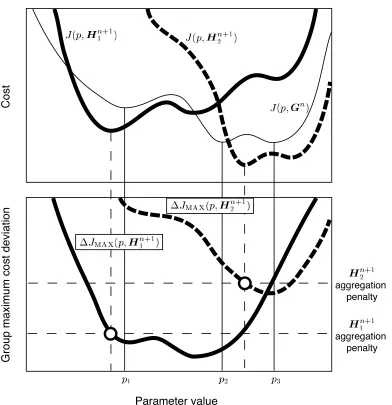
The behaviour of the station aggregation procedure at the nth step is illus-trated in Fig. 1 for a simple case where the model has only one parameter. The figure shows how the procedure chooses between two groupsHn+1

1 andHn2+1.

The group which we aim to select is that with the lowest aggregation penalty, defined with reference to the group’s cost function minimum. Comparison of the aggregation penalties shows that Hn+1

1 is the true optimal group.

How-ever, in practice the aggregation penalties are unknown because minimization of the cost function for all possible groups is too expensive. In the absence of information regarding the location of each group’s cost function minimum, the group maximum cost deviation, designed for selecting between groups, has the additional function of acting as a proxy for the cost function in parameter space. While its variation in parameter space is broadly similar to that of the cost function, there are differences because it is sensitive to different model output: the group maximum cost deviation is sensitive to output at the station least favoured for inclusion in the group, whereas the cost function might be particularly sensitive to output at another station, such as the station with the most reliable observations. The implications of this are discussed in Appendix A.

The main limitation is that it is only possible to evaluate the group maxi-mum cost deviation at a relatively small number of points in the parameter space. The set of sample points in parameter space, the search set P_{, is} de-termined with reference to the cost function for the optimal group of size n, Gn_{. The underlying assumption is that the set} P_good(Gn_{) is, by virtue of its} pre-conditioning, sufficiently representative of the most promising areas of pa-rameter space for a similar but slightly larger group to allow the best such group to be selected. For the example in Fig. 1, there are three parameter values in P _{within the region of interest,p1, p2 andp3. The lowest point} sam-pled on either of the group maximum cost deviation curves lies on that for group Hn+1

1 at p2. The selection is therefore successful. Examples are given

in Appendix A where this is not the case, to illustrate the limitations of the method.

To start the procedure, rather than choosing an arbitrary station s and re-stricting the initial set of parameter vectors P_{init to} P_{good(s), we aim for a} more robust result by pooling the sets of parameter vectors obtained by opti-mizing for all stations individually. This increases the initial number of trial parameter vectors by a factor equal to the number of stations in the calibration set.

suitabil-Parameter value

Cost

Group maximum cost deviation

aggregation penalty

aggregation penalty

Fig. 1. Behaviour of the station aggregation procedure at step n for a single pa-rameter model. The group with the lower aggregation penaltyHn+1

1 is successfully identified as a result of sampling the cost deviation curves for the two groups atp1,

p2 andp3.

error, is introduced in Section 2.5.

2.4 Identification of provinces and calibration groups

The calibration algorithm is implemented by two fundamental procedures, both of which invoke the station aggregation procedure. The first of these is the ‘whole-domain calibration procedure’, which seeks the optimum group of stations for a single-parameter vector calibration of a given geographic domain. The second is the ‘split-domain calibration procedure’, which seeks optimal station groups for a two-parameter vector calibration of the domain. Any aggregation group which shows good geographic coverage of some province within the domain can serve as a starting point for this procedure. Such groups are referred to as province indicator groups. Each aggregation group of suit-able size identified during the application of the whole-domain calibration procedure to the domain is a potential candidate. These candidate groups are assessed with regard to the geographic distribution of their member stations, ignoring any with less than 3 stations or any which leave less than 3 stations remaining in the domain’s calibration set. A single province can include mul-tiple regions of the domain, each represented by at least 3 stations, allowing for the possibility that geographically separated regions might share similar ecological responses to environmental forcing.

For any given domain, one application of the whole-domain calibration pro-cedure is required, followed by zero or more applications of the split-domain calibration procedure, depending on the number of province indicator groups found. The split-domain calibrations are evaluated against each other and against the whole-domain calibration by comparing the costs of the calibrated model with respect to the domain’s validation data. If the best calibration is a split-domain calibration then the associated provinces define two new domains to which the calibration algorithm is applied recursively.

2.4.1 Whole-domain calibration procedure

In the whole-domain calibration procedure, a trial optimization is first done using all stations in the domain’s calibration setD_{. The best parameter vector} thus obtained~pBEST(D) is evaluated by running the model at all stations in the

validation set V _{to obtain the validation cost J{~pBEST(}D_),V_{}. The station} aggregation procedure is then applied to the stations in D_{, giving a series} of alternative calibration groups Gi_{, of increasing size i, The validation cost}

J{~pBEST(Gi),V}is determined for each of these groups. All of the validation

of the aggregation groups (C ₌ Gi _{for some i). The validation cost for the} whole-domain calibration is J{~pBEST(C),V}. The set of province indicator

groups is formed from all suitable aggregation groups.

2.4.2 Split-domain calibration procedure

The split-domain calibration procedure splits the domain into two provinces using, as a starting point, a specific province indicator group G_{A (}G_{A =} Gi for somei). The associated province is referred to as the primary province A. The remainder of the domain is referred to as the complementary provinceB. Any single stations or pairs of stations which are geographically isolated by the province indicator groupG_{A cannot be considered indicative of a separate} region. They are therefore considered to be atypical stations in province A

rather than province B stations.

Geographic borders are established between the two provinces, allowing the validation set V _{to be split into separate sub-sets} V_{A and} V_{B for each} province. The full calibration set D _{is likewise split into sub-sets} D_{A and} D_{B. In the present study, lines of latitude were used where possible and,} where calibration stations at the same latitude fell in different provinces, in-tervening validation stations were assigned such that there was at least one validation station at the same latitude in each province if possible.

Calibration groups C_{A and} C_{B are identified by applying the whole-domain} calibration procedure to each of the provincial calibration sets D_{A and} D_B. For province B, this involves another application of the station aggregation procedure. For provinceA, the previous aggregation results can be used. How-ever, if there are stations in the calibration setD_{A which are not in the group} G_{A, the aggregation procedure must be repeated, starting from}G_{A, to check} whether the series of aggregation groups can be extended within province A. This may now be possible as a consequence of the exclusion of stations outside

Afrom the calibration set. The validation cost for the split-domain calibration

JSPLIT_{~p

BEST(CA),VA, ~pBEST(CB),VB}

2.5 Allowing for observation error

Estimates of observation error provide valuable information for any data as-similation scheme, their principal use being to weight the model misfit to individual observations such that higher precision observations have a greater influence on the model. Taking observation error into account also allows sta-tistical significance to be associated with differences in the misfit cost between different model integrations. This allows the cost deviation for a station to be redefined in terms of a statistic for significance testing. It also allows the significance of differences in validation cost to be taken into account when comparing alternative model calibrations for a domain.

2.5.1 Model misfit

The misfit is defined here in terms of the squared deviation of the model from the observation, weighted according to the observation variance. While this is a useful definition which is consistent with previous work, other definitions of model misfit could be used. The misfit of the model with parameter vector ~p

with respect to the ith observation from the setX _{at thejth station is given} by

Mij(~p,X) =

{xijMODEL(~p)−xijOBS}2

var(xijOBS)

(4)

where the subscripts ‘MODEL’ and ‘OBS’ denote model predictions and ob-served values of x (x ∈ X_{) respectively. Each observation xijOBS is the} ex-pected value of X_{, for a particular time and location, derived from} obser-vational data. This is the estimated mean of a population of possible values affected by both measurement and sampling error. The population variance quantifies the observation error due to the combined effect of these sources. Division by an estimate of the variance var(xijOBS) non-dimensionalizes the

misfit so that a misfit of unity or less implies a model deviation not exceeding the observation error.

2.5.2 Cost function probability distribution

observations. Observational uncertainty is represented by a joint probability distribution in a multi-dimensional space having one dimension for each avail-able observation. For any group of stations, the cost distribution is defined by the application of the cost function to the appropriate lower-dimensional subset of this observation distribution.

To derive an estimate ˆJ _{of a particular cost distribution} J_{, the cost function} is applied to a sample of observation vectors drawn from a probability distri-butionΩ: a model of the observation probability distribution. Its multivariate mean is the vector of expected observation values xijOBS, while its variance

structure is chosen to be consistent with the estimated observation error. The observation error at each time and location is assumed to have a normal dis-tribution with zero mean and variance equal to the estimate var(xijOBS). Error

covariances between stations are assumed to be zero. This is implicit in the method because it must be possible to evaluate costs at stations individually. In the present work, the errors are also assumed to be temporally independent so that all error covariances are zero. The univariate observation distribution for the ith observation from the data set X _{at the jth station is therefore} given by

Ωij(X) =xijOBS+E q

var(xijOBS) (5)

where E _{is the normal distribution with zero mean and unit variance. Ωij is} substituted for the expected observation value in the misfit expression from Eq. (4) to give a misfit probability distribution

M_ij(~p,X_{) =} {xijMODEL(~p)−Ωij(X)}

2

var(xijOBS)

(6)

This is substituted for the misfit Mij in the cost function to define the cost probability distributionJ_.

2.5.3 Modification of the station aggregation procedure

The new cost deviation for a parameter vector ~p at station s, taking into account observation error, is the test statisticU(~p, s) derived by comparing the cost distribution estimate ˆJ_{(~p, s) with the station’s baseline cost distribution} estimate ˆJ_{(~pBEST(s), s). Substituting for the cost deviation ∆J in Eq. 2 gives} the new aggregation penalty for a group Hn

UMAX{~pBEST(Hn),Hn}=

n max

i=1 {U(~pBEST(

Hn_{), si)}. (7)}

The station aggregation procedure, defined in Section 2.3, is modified by re-placing the old cost deviation ∆J(~p, s) with U(~p, s) and the old group max-imum cost deviation ∆JMAX{~p,HnBEST+1 (~p)} with UMAX{~p,HnBEST+1 (~p)}.

Unfor-tunately, a complication arises because infinite values of the cost deviation

U(~p, s) occur if there is no overlap between the two cost distribution esti-mates. In that case, the parameter vector ~p has no measurable merit with respect to the stations data and the station is considered to be ‘not satisfied’ by the parameter vector. The existence of such stations introduces an ad-ditional termination condition for the station aggregation procedure. It may now terminate, at any stepn, if no group of the required sizen+ 1 is satisfied by any of the available parameter vectors in the current search set P_{. That} is if, for all ~p ∈ P_{, there are less than n + 1 stations s (s ∈} D_{) with finite}

U(~p, s), so that the group Hn+1

BEST(~p) cannot be formed. Early termination of

the station aggregation procedure saves on computation time and could be introduced with the original cost deviation definition for this purpose, by set-ting an upper limit to ∆J. However, it does introduce a complication which must be allowed for in the split-domain calibration procedure as described in the next section.

2.5.4 Modification of the calibration algorithm

In the calibration algorithm, shown in its final form in Fig. 2, comparisons be-tween alternative model calibrations are now made with reference to the me-dian values of their validation cost distribution estimates and the split-domain calibration procedure is modified to allow for provinces with incomplete sta-tion aggregasta-tion.

provinces (if any)

calibration group(s) & parameter vector(s) validation cost distribution

whole-domain calibration

split-domain calibration

select best calibration

split-domain calibration

Fig. 2. The calibration algorithm used to identify the optimum calibration for a given domain having the set of calibration stations D_{. (See text for details.)}

split-domain cost distribution estimate

ˆ

JSPLITn_~pBEST(C_A[j]),V_{A[j], ~pBEST(}C_B[j]),V_B[j]o

with the lowest median is identified and compared with the whole-domain cost distribution estimate. If it is significantly lower, at a probability of 95%, then the split-domain calibration is accepted. Otherwise the whole-domain calibration is accepted.

The requirement for modifying the split-domain calibration procedure arises because, for symmetry, the geographic border or borders between the two provinces A and B should be drawn between two aggregation groups. We cannot now assume that all stations in the complementary province B will aggregate. If they do not, there may be a gap between the aggregation groups and an adjustment may need to be made to the border so that it bisects this unrepresented area or otherwise divides it in a sensible way.

The modified split-domain calibration procedure is shown in Figure 3. Prior to any border adjustment, the provinces are now referred to as the poten-tial primary province Apot and the potential complementary province Bpot. The station aggregation procedure is applied to the set of calibration stations withinBpot, denotedD_{Bpot. Unless forced to terminate early, the aggregation} procedure normally terminates when the group GN−1 _{is found, where N is}

the size of the calibration set. However, in this case, there is a requirement to know whether the full calibration set D_{Bpot is also an aggregation group. The} procedure is therefore extended to test whether the final station would aggre-gate. That is, whether it is satisfied by a parameter vector in the search set P_good(GN−1_{). The largest aggregation group obtained G}

B is used, together withG_{A, to define the border or borders between the final provinces AandB.} The whole-domain calibration procedure is then applied toAandB as before. For province B, this now only involves determining the validation costs. For provinceA, extension of the series of aggregation groups beyondG_{Amay also} be required.

3 Testing the method

define provinces

Apot and

Bpot

aggregate stations

define provinces

A and B

whole-domain calibration

whole-domain calibration

validate

Fig. 3. The procedure for obtaining the optimum split-domain calibration based on a given province indicator groupG_{A. (See text for details.)}

any at which there were obvious problems with the model’s external forcing data. Only about half were used. These 30 remaining stations are divided into calibration and validation sets of 15 stations each.

depends on the finite sample of parameter vectors available from the individual station optimizations and alternative samples could result in the selection of different pairs. To test the robustness of the results to the selection of the ini-tial pair, additional aggregation experiments were performed with alternative pairs.

3.1 Observations

The observed variables used in this test are from two data sets: logC_{, where}C

is the set of chlorophyllaconcentrations, and the set of annual nitrate concen-tration maxima N_{. Although the surface layer chlorophyll data derived from}

satellite ocean colour are invaluable because of their good spatial and tempo-ral coverage, they provide information relating to one ecosystem component only and this is recognized as a major limitation. Climatological estimates of the annual maximum nitrate concentration in the upper mixed layer therefore provided a useful additional constraint. Seasonal estimates of mixed layer ni-trate concentration are available but were not used in the present study. This is partly because they are much less reliable than the annual maxima, being especially prone to sampling error associated with interannual variability, but also because their comparison with the output available from the candidate model is not straightforward. The latter problem is explained in Section 3.3. Observational nitrate estimates are the only relevant in situ data presently available for the whole basin. Otherin situ data are only available at isolated locations and were not used.

The resolution of the data should reflect the application for which the model is to be evaluated. We envisage a hypothetical target application requiring field predictions down to time scales of the order of 1 day and space scales of 200 km. The observed mean and variance estimates of logC _and N _required

for the cost function are therefore those describing data distributions over a 200 km length scale. This is considered to be sufficiently large to prevent major problems with aliasing due to mesoscale eddy activity. Any observation within 100 km of a station is treated as a possible realization of the true value at the station location. Chlorophyll data from a specific year were used, in preference to climatological values, to avoid the potentially serious loss of information which can result from combining multiple annual cycles in which phytoplankton blooms are out of phase.

All chlorophyll a estimates within 100 km of the nominal station positions were extracted from daily SeaWiFS 9 km Standard Mapped Image data for 1998, this being the first complete calendar year of data available. logC _was

pixels being weighted by area to allow for meridional variation. The variance quantifies the observation error, which is a combination of the measurement er-ror associated with the SeaWiFS Chlorophyll estimates (±35%) and sampling error associated with mesoscale variability. To avoid bias due to poor cover-age, samples of less than 10 pixels and samples with a standard deviation in meridional or zonal position of less than 30 km were not used. A sample giving complete coverage has a standard deviation of 50 km. The log transformation is required to give a pseudo-normal distribution. This was tested by examining combined probability density functions forC _{and log}C _{for observations at all}

times and all stations. It is also supported by theoretical considerations and other empirical data (Campbell, 1995).

The nitrate maximum normally occurs in late winter as a result of deep winter-time mixing. Observed values of N _{were estimated, following the method of}

Glover and Brewer (1988), by interpolating vertical nitrate profiles, extracted from World Ocean Atlas (WOA) 1◦ _{analyzed annual mean fields (Conkright et}

al., 1998), to the average depth of the mixed layer over the period February-April. Where this depth is greater than 500 m, the concentration at 500 m was used. The average mixed layer depth was estimated from averaging monthly data on a 1◦ _{grid. The mixed layer depth estimates of Levitus et al.}

(1982) based on a density difference criterion (∆σt= 0.125) were used as these are readily available. The processing differs slightly from that of Glover and Brewer (1988) who averaged winter-time hydrographic profiles (Levitus et al., 1982) over the 3 month period before calculating mixed layer depth using a variable σt criterion. Their criterion was equivalent to a 0.5◦C temperature criterion in the absence of salinity stratification. Despite these differences in processing, the resulting winter-time mixed layer depth fields are very similar, with the exception of a few northern regions above 55◦_{N where the use of the}

fixed σt criterion gives some exceptionally high values. The cut off at 500 m means that this has little effect on the nitrate maximum estimates. Nitrate values obtained where the winter-time mixed layer depth is less than 100 m are considered unreliable because of the likelihood of strong seasonal bias in the nitrate concentrations observed above this depth. These were therefore omitted.

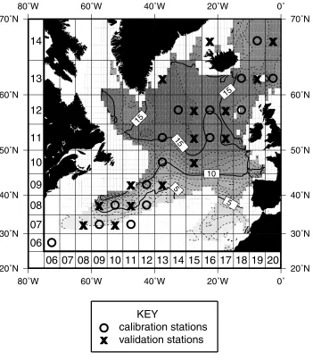
The estimated annual nitrate maximum field is shown in Fig. 4, together with the calibration and validation stations. For ease of reference, stations are numbered according to their grid position in the format YYXX. They are assigned alternately to calibration and validation sets in numerical order. To obtain the estimates of the 200 km scale mean for the cost function, the winter-time nitrate field was averaged over 3◦_{boxes centred on station locations. This}

80˚W 80˚W

60˚W 60˚W

40˚W 40˚W

20˚W 20˚W

0˚ 0˚

20˚N 20˚N

30˚N 30˚N

40˚N 40˚N

50˚N 50˚N

60˚N 60˚N

70˚N 70˚N

06 07 08 09 10 11 12 13 14

06 07 08 09 10 11 12 13 14 15 16 17 18 19 20

5

5

10

15

15

15

KEY

calibration stations validation stations

Fig. 4. Estimated annual maximum nitrate concentration in the mixed layer (mmol m−3_{) and distribution of calibration and validation stations. Each station is} iden-tified by a four digit station number of the form YYXX, formed by concatenating the 2 digit meridional and zonal position numbers shown on the grid.

were discarded. In the absence of information about the variance of the nitrate maximum at the 200 km scale it’s standard deviation was somewhat arbitrarily set to 1 mmol m−3 _{for all stations.}

Five of the stations have no nitrate observation. These are 0606 (27.5◦_N

72.5◦_{W), 0711 (32.5}◦_{N 47.5}◦_{W), 0911 (42.5}◦_{N 47.5}◦_{W), 1313 (62.5}◦_{N 37.5}◦_W)

and 1416 (67.5◦_{N 22.5}◦_{W). Two of these stations are in the calibration set.}

3.2 Cost function

The cost function returns the sum of the misfit costs for each of the observed variables

J =Jchl+Jnit (8)

The chlorophyll misfit cost for parameter vector ~p and group H _{is the mean} misfit for logC _{over all stations and observation times. So}

Jchl(~p,H) =

Pn

j=1

Pnj

i=1Mij(~p,logC)

Pn

j=1nj

(9)

where n is the number of stations in H _{and nj is the number of chlorophyll} observations for the jth station, which varies largely due to cloud cover. The nitrate misfit cost is the mean misfit for N _{over all stations}

Jnit(~p,H) =

1

n

n

X

j=1

Mj(~p,N) (10)

For the purposes of constructing the simulated observation probability distri-bution Ω, logC _and N _{were treated as a single data set. Each observation}

vector in the sample drawn from Ω for the cost distribution estimates com-prises N nitrate values and PN

j=1nj chlorophyll values, where N is the total number of stations in the calibration and validation sets. i.e. N = 30.

3.3 Model

The model’s external forcing data includes spatially varying annual cycles of day length, photosynthetically available radiation (PAR), mixed layer depth and phytoplankton maximum growth rate modelled as a function of tempera-ture. These are augmented by spatially varying annual mean nitrate profiles, which define the sub-surface nitrate at the base of the mixed layer. While there are no explicit horizontal fluxes, keeping the sub-surface nitrate profiles con-stant implicitly includes the effect of horizontal nitrate fluxes on time scales longer than a year.

Year-specific satellite data for 1998 were used to define the PAR and tem-perature cycles but were not available for mixed layer depth and nitrate. Cli-matological mixed layer depth and nitrate fields were therefore substituted. A consequential limitation of the model is that the temporal resolution of its mixed layer depth forcing data is inconsistent with the requirements of the hy-pothetical target application for which it is being evaluated. Mixed layer depth data from a climatological integration of a 3-dimensional general circulation model (see Appendix B) were used in preference to observational estimates. Use of model data is prudent because the observational estimates available do not sufficiently resolve the rapid shoaling of the mixed layer in the spring. To minimize problems due to incorrect timing of spring shoaling in the sim-ulation, surface layer temperature cycles from the simulation were screened against the 1998 temperature observations and stations where the model and observations appeared to be out of phase were excluded. For the remaining stations, the mean winter-time (February-April) mixed layer depth from the simulation is compared with the observational estimate used to determine the annual nitrate maximum (Fig. 5). With the exception of some of the northern values, where the observational estimate is high as a result of the fixedσt cri-terion, there is generally good agreement between the two estimates, although the simulated values do show a high bias. Full details of the model’s external forcing data are given in Appendix B.

0

200

400

600

800

1000

0

200

400

600

800

1000

Observed MLD (m)

Sim

ulated MLD (m)

Fig. 5. Mean simulated mixed layer depth for the period February-April from the general circulation model compared with observational estimates for the same pe-riod. The latter are derived from the 1◦ _{monthly data of Levitus et al. (1982), based} on a density difference criterion ∆σt= 0.125. The 1:1 line is shown for reference.

4 Results

The results of applying the split-domain calibration method as defined in Section 2 to the PZN model are described here. The results of the robustness experiment are given in Appendix C.

4.1 Calibration domains

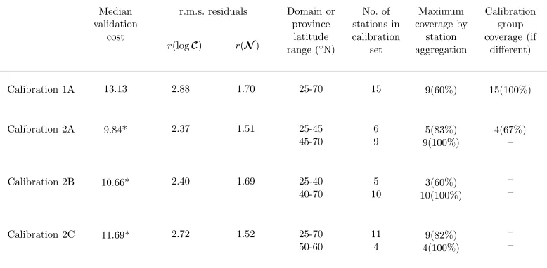
Table 2

Summary of calibration results for the North Atlantic domain

Median validation

cost

r.m.s. residuals

r(logC) r(N)

Domain or province

latitude range (◦_N)

No. of stations in calibration set Maximum coverage by station aggregation Calibration group coverage (if different)

Calibration 1A 13.13 2.88 1.70 25-70 15 9(60%) 15(100%)

Calibration 2A 9.84* 2.37 1.51 25-45 45-70 6 9 5(83%) 9(100%) 4(67%) –

Calibration 2B 10.66* 2.40 1.69 25-40 40-70 5 10 3(60%) 10(100%) – –

Calibration 2C 11.69* 2.72 1.52 25-70 50-60 11 4 9(82%) 4(100%) – –

Validation costs for split-domain calibrations which are significantly lower (at 95%) than that for the whole-domain calibration (Calibration 1A) are marked *. Coverage of the domain or province is expressed in terms of the number of calibration stations and, in brackets, the proportion of the domain or province this represents.

costs are the medians of the distributions

ˆ

J_{~pBEST(C_),V_}

and

ˆ

JSPLITn_~pBEST(C_A[i]),V_{A[i], ~pBEST(}C_B[i]),V_B[i]o

for the whole-domain calibration and the ith split-domain calibration respec-tively. The root mean square residuals for the chlorophyll and nitrate valida-tion data are also shown. These are the residuals with respect to the observa-tion means, given by:

r(logC_{) =} v u u t Pn j=1

Pnj

i=1Mij(~pj,logC)

Pn

j=1nj

(11)

and

r(N_{) =} v u u t 1 n n X j=1

Mj(~pj,N) (12)

applicable to thejth station. The residual values are dimensionless, each refer-ring to a number of standard deviations of the error distribution estimate for the observation. However, for nitrate, a constant observation error estimate with a standard deviation of 1 mmol m−3 _{is used throughout the domain, so}

the values are equivalent to concentrations expressed in mmol m−3_.

Latitude ranges are given in the table for each domain or province. The provin-cial latitude ranges are for identification purposes and do not constitute com-plete province descriptions. The actual geographical extent of each province is shown in Fig. 6. The maximum coverage of the domain or province by station aggregation indicates how representative the largest aggregation group from the applicable whole-domain calibration is of the full calibration set. A cover-age of 100% implies that the largest aggregation group is effectively the full calibration set. This means that the station aggregation procedure completed successfully and that the single remaining station is satisfied by a parameter vector in the final search set. The omission of a small proportion of the calibra-tion set’s stacalibra-tions is acceptable: the omitted stacalibra-tions are considered atypical. However, in some cases the coverage is as low as 60%, calling into question the applicability of the aggregation result to the whole domain or province. The calibration group referred to in the table is usually the largest aggregation group. However, as indicated in Section 2.4.1, it can be one of the smaller groups if the optimal parameter vector for that group gives a lower validation cost. It can also be the full calibration set, irrespective of whether this qual-ifies as an aggregation group. Where the calibration group is not the largest aggregation group, its coverage is given as a separate entry in the table.

The whole-domain calibration result for the North Atlantic domain is referred to as Calibration 1A, where 1 denotes the number of parameter vectors re-quired to cover the domain. This is based on the full 15 station calibration set. When the station aggregation procedure was applied, the maximum num-ber of stations aggregated was only 9 out of 15. The calibration based on the 9 station group gives a median validation cost of 14.34, which is lower than those for the smaller groups but higher than that for the full calibration set.

80°W 60°W 40°W 20°W 0° 20°N 20°N 30°N 30°N 40°N 40°N 50°N 50°N 60°N 60°N 70°N 70°N 06 07 08 09 10 11 12 13 14

06 07 08 09 10 11 12 13 14 15 16 17 18 19 20

SARC ARCT NADR NAST(E) NAST(W) GFST

(a)

06 07 08 09 10 11 12 13 14 15 16 17 18 19 20

SARC ARCT NADR NAST(E) NAST(W) GFST

(b)

80°W 60°W 40°W 20°W 0°

20°N 20°N 30°N 30°N 40°N 40°N 50°N 50°N 60°N 60°N 70°N 70°N 06 07 08 09 10 11 12 13 14

06 07 08 09 10 11 12 13 14 15 16 17 18 19 20

SARC ARCT NADR NAST(E) NAST(W) GFST

(c)

KEY calibration stations used calibration stations not used validation stations

and Station 0711 (32.5◦_{N 47.5}◦_{W), are excluded from the calibration groups in}

all of the split-domain calibration results. This demonstrates that the method is able to allow for atypical stations.

Shown for reference in Fig. 6 are the divisions between the oceanic biogeo-chemical provinces defined by Longhurst (1998). In Calibration 2A, the divi-sion between the provinces is coincident with the boundary between the North Atlantic Drift Province and the North Atlantic Subtropical Gyral Province. This is consistent with the idea that model parameters should at least be invariant within the pre-defined biogeochemical provinces. The second best split-domain calibration, Calibration 2B, is very similar to the first and al-though the division is slightly further south it too coincides with pre-defined biogeochemical province boundaries. In the last split-domain calibration, Cal-ibration 2C, one of the provinces is geographically divided such that northern and southern regions share the same parameter vector, while a mid-latitude region forms the alternate province. There is no clear relationship between these provinces and the pre-defined biogeochemical provinces.

Although there are obvious advantages in combining stations when calibrat-ing a model for application to a wide area, the benefits are less clear for local studies in which a model is required to produce time-series estimates for a single location. In that case, we might expect local calibrations to have greater relevance. It is therefore informative to compare the calibrated model’s goodness-of-fit at the validation stations with that obtained by extrapolating individual station calibrations locally.

Local calibrations were tested at each of the 15 validation stations in the domain by applying the optimal parameter vector for the nearest calibration station at the same latitude. Where stations were equally close geographically, that with the closest nitrate observation value was chosen. Stations with no nitrate data were ignored. The median validation cost for the North Atlantic domain based on these local, single-station calibrations is 12.92. While the median cost for the whole-domain calibration (Calibration 1A) is higher than this, the costs for all 3 of the split-domain calibrations (2A, 2B and 2C) are significantly lower (at 95%), with reductions of up to 24% (Calibration 2A).

uncorrelated between adjacent stations, so that the observations at each can be treated as independent samples of the annual chlorophyll cycle, the cycles themselves tend to be correlated between stations. The power of the validation data to test the generality of the calibrated model is to some extent compro-mised by this. In general, correlation between observations at validation and calibration stations will tend to introduce an unwanted bias towards the selec-tion of smaller provinces, since a combinaselec-tion of the model’s descriptive and predictive abilities are tested, rather than purely its predictive skill. It is there-fore not possible to determine whether the favourable local parameter vectors reflect true local biogeochemical characteristics or are simply compensating for deficiencies in the model. In general, the single-station calibrations seem unreliable and the results presented here clearly demonstrate the advantage of combining multiple stations for local as well as basin-scale applications.

4.2 Spatial distribution of model error

The spatial distribution of the model misfits are summarized by maps of the station r.m.s. model residual for chlorophyll, defined at the jth station by

rj(logC) =

v u u

t 1

nj

nj

X

i=1

Mij(~pj,logC) (13)

and the nitrate residual

εj(N) = νjMODEL(~pj)−νjOBS (14)

where ν ∈ N_{. These are presented here (Fig. 7 and 8) for the whole-domain}

calibration (Calibration 1A) and for each of the split-domain calibrations (Cal-ibrations 2A, 2B and 2C).

The chlorophyll error map for the whole-domain calibration (Fig. 7a) shows an approximate r.m.s. residual of between 2 and 4 observational standard devia-tions, representing a rather poor fit throughout the domain. The correspond-ing map for nitrate (Fig. 8a) shows that the winter-time nitrate maximum is underestimated everywhere by the model with the exception of Station 1319 (62.5◦_{N 7.5}◦_{W). The magnitude of the error is 2 mmol m}−3 _{or less almost}

everywhere though, which is relatively small compared with the chlorophyll error, based on the assumption implicit in the cost function of a 1 mmol m−3

error in the observational nitrate estimate.

80°W 80°W 60°W 60°W 40°W 40°W 20°W 20°W 0° 0° 20°N 30°N 40°N 50°N 60°N 70°N 3

2 2 3 2 3 4 3 3

2 3 2

3 3

4 3 3 3 4 3 3 3 3

3 2 2 2

3 3 3

06 07 08 09 10 11 12 13 14

06 07 08 09 10 11 12 13 14 15 16 17 18 19 20

(a)

2 2 3 2 3 3 2 2

3 3 2 3 2 2 2 2 2

2 2 2 4 3

2 2 1 1

2 2 3

06 07 08 09 10 11 12 13 14

06 07 08 09 10 11 12 13 14 15 16 17 18 19 20

(b)

2 2 3 2 3 2 2 2

2 3 3

3 2

3 2 2 2 3 2 2 3 2

2 2 1 2

2 3 4

06 07 08 09 10 11 12 13 14

06 07 08 09 10 11 12 13 14 15 16 17 18 19 20

(c)

2 2 3 2 3 3 3 3

2 2 2 3 4 1 1 1 2

2 1 2 3 3

4 2 2 3

3 3 4

06 07 08 09 10 11 12 13 14

06 07 08 09 10 11 12 13 14 15 16 17 18 19 20

(d)

Fig. 7. Approximate station r.m.s. residual for chlorophyll rj(logC), in number of

standard deviations, for (a) Calibration 1A, (b) Calibration 2A, (c) Calibration 2B and (d) Calibration 2C. Circled stations are the calibration stations used. The extent of each province is indicated by the shading.

deviations (Fig. 7b-d). In Calibration 2A, there is some tendency for chloro-phyll errors to be lower in the northern province than in the south. Almost everywhere in this northern province the fit to chlorophyll is better than in Calibration 1A, while the nitrate errors (Fig. 8b) are very similar.

vari-80°W 80°W 60°W 60°W 40°W 40°W 20°W 20°W 0° 0° 20°N 30°N 40°N 50°N 60°N 70°N

-1 -1 -1 -2 -2 -2 -1

-2 -2 -2 -2 -2 0 0 -2

-1 -1 -1 0 0 -1 3 -1

-1 -2 06 07 08 09 10 11 12 13 14

06 07 08 09 10 11 12 13 14 15 16 17 18 19 20

(a)

-1 -1 -1 -1 -1 -1 0

-1 -2 -2 -1 -2 0 0 -2

-1 -1 -1 0 0 -1 3 -1

-1 -2 06 07 08 09 10 11 12 13 14

06 07 08 09 10 11 12 13 14 15 16 17 18 19 20

(b)

-1 -1 -1 -2 -2 -2 -1

-2 -2 -1 -1 -1 0 0 -2

-1 -1 -1 0 0 0 4 -1

-1 -1 06 07 08 09 10 11 12 13 14

06 07 08 09 10 11 12 13 14 15 16 17 18 19 20

(c)

-1 -1 -1 -2 -2 -1 0

-1 -2 -1 -1 -1 1 1 -1

-1 0 0 0 0 -1 3 -1

-1 -2 06 07 08 09 10 11 12 13 14

06 07 08 09 10 11 12 13 14 15 16 17 18 19 20

(d)

Fig. 8. Approximate nitrate residualεj(N) (mmol m−3) for (a) Calibration 1A, (b)

Calibration 2A, (c) Calibration 2B and (d) Calibration 2C. Circled stations are the calibration stations used. The extent of each province is indicated by the shading.

the presence of larger blooms and more pronounced seasonal variation allow the functions describing the processes in the model to be sensibly constrained over a greater dynamic range.

4.3 Parameters

Unless parameters are well constrained by the observations, cost values which are only slightly higher than the lowest found JBEST can occur over large

areas of the parameter space. In many cases, an optimization result is therefore better represented in the form of a joint probability distribution for the optimal parameter values, rather than by a single vector. This posterior parameter distribution contains information about the degree of parameter constraint achieved as well as the correlation between different parameters. An estimate of the posterior parameter distribution can be derived fromP_{goodby removing} outliers associated with unacceptably high costs, as done by Schartau et al. (2001). However, the definition of an unacceptably high cost is somewhat arbitrary. Accepting a wide range of costs increases the likelihood of including sub-optimal parameter vectors, while restricting the range reduces the size of the sample so that it becomes less representative of the distribution in parameter space of possible global minima. Schartau et al. (2001) defined costs within 25% of JBEST as acceptable. A statistical approach is used here, which

takes into account the observation error by making use of cost probability distribution estimates determined for each parameter vector, in place of single cost values. An unacceptably high cost distribution is defined as one which differs significantly from that with the lowest median at a chosen level of probability.

province sample of 13 parameter vectors is 7.78 to 8.25. The upper costs for southern and northern provinces are 9% and 6% higher than the lowest costs respectively. These cost ranges are small compared with the 25% cost differ-ence considered acceptable by Schartau et al. (2001). However, relatively small cost differences are highly significant here as a consequence of averaging over a large number of observations.

The univariate posterior parameter distribution estimates for the accepted cal-ibration are shown in Fig. 9. These are the projections of the joint probability distribution estimates onto the parameter axes. In the case of both southern and northern calibrations, most parameters appear poorly constrained. There is evidence (not presented here) to suggest that some parameters may be much better constrained by the observations at a probability of 95%. However, this is based on sample sizes of just 3 for each province and cannot therefore be considered very reliable.

In some cases, parameters can be difficult to constrain because their optimal values are not independent. This is reflected by non-zero covariances in the pos-terior probability distributions. Parameter dependencies were investigated by calculating the Pearson correlation coefficients for all possible parameter pairs in each sample. In contrast with techniques used by other workers (Matear, 1995; Fennel et al., 2001), which are based on analysis of the Hessian matrix of the cost function at its minimum, our statistical approach is global with respect to the parameter space, allowing for the existence of multiple minima within the acceptable cost range.

Large positive and negative correlation coefficients were found for a number of the parameter pairs, the most notable of which are consistent between the independent results for southern and northern provinces. These are the two largest negative correlations and the largest positive correlation found in each case. The correlated parameters are the zooplankton ingestion half-saturation constant kG and the chlorophyll to nitrogen ratio χ (correlation coefficients

of -0.76 and -0.74 for the southern and northern provinces respectively), the zooplankton excretion rateµand the chlorophyll to nitrogen ratio (0.70 and -0.63) and the zooplankton excretion rate and the cross-pycnocline mixing rate

m(+0.84 and +0.63). It is difficult to see any clear reasons for these parameter pairs to be correlated in reality and the relationships may be a consequence of unrealistic constraints imposed by the model design and/or forcing data.

Despite the uncertainty in parameter values, the posterior parameter distri-butions show some interesting patterns. Estimates of phytoplankton specific mortality φP are consistently low, suggesting that phytoplankton mortality is

ex-0 20 40 60 80 100

0 2 4 6 8 10

m (m d-1₎

Frequency (%

) PRIOR

0.5 1.0 1.5 2.0 2.5 3.0

χ (g mol-1₎

PRIOR

0.00 0.02 0.04 0.06 0.08 0.10 kchl (m2mg-1)

PRIOR

0 20 40 60 80 100

0.0 0.1 0.2 0.3 0.4

α (d-1_{(W m}-2₎-1₎

Frequency (%

) PRIOR

0.2 0.4 0.6 0.8 1.0 kN (mmol N m-3)

PRIOR

0.00 0.05 0.10 0.15 0.20 0.25 0.30

φP (d-1)

PRIOR

0 20 40 60 80 100

0.0 0.5 1.0 1.5 2.0 2.5 3.0 g (d-1₎

Frequency (%)

PRIOR

0.5 1.0 1.5 2.0 2.5 3.0 kG (mmol N m-3)

PRIOR

0.0 0.2 0.4 0.6 0.8 1.0

β

PRIOR

0 20 40 60 80 100

0.0 0.1 0.2 0.3 0.4 0.5

µ (d-1₎

Frequency (%)

PRIOR

0.00 0.05 0.10 0.15 0.20 0.25 0.30

φZ ((mmol N m-3 d)-1)

PRIOR

0.0 0.2 0.4 0.6 0.8 1.0

PRIOR

KEY southern province northern province