An adaptive bilateral negotiation model for e commerce settings

An Adaptive Bilateral Negotiation Model for E-Commerce Settings

Vidya Narayanan and Nicholas R. Jennings

Intelligence, Agents, Multimedia

School of Electronics and Computer Science

University of Southampton SO17 1BJ, UK.

{

vn

03

r, nrj

}@

ecs.soton.ac.uk

Abstract

This paper studies adaptive bilateral negotiation between software agents in e-commerce environments. Specifically, we assume that the agents are self-interested, the environ-ment is dynamic, and both agents have deadlines. Such dynamism means that the agents’ negotiation parameters (such as deadlines and reservation prices) are functions of both the state of the encounter and the environment. Given this, we develop an algorithm that the negotiating agents can use to adapt their strategies to changes in the environ-ment in order to reach an agreeenviron-ment within their specific deadlines and before the resources available for negotia-tion are exhausted. In more detail, we formally define an adaptive negotiation model and cast it as a Markov Deci-sion Process. Using a value iteration algorithm, we then in-dicate a novel solution technique for determining optimal policies for the negotiation problem without explicit knowl-edge of the dynamics of the system. We also solve a repre-sentative negotiation decision problem using this technique and show that it is a promising approach for analyzing ne-gotiations in dynamic settings. Finally, through empirical evaluation, we show that the agents using our algorithm learn a negotiation strategy that adapts to the environment and enables them to reach agreements in a timely manner.

1. Introduction

Automated negotiation is a key issue for e-commerce be-cause it provides the de facto means of interaction between stakeholders with different aims and objectives [4]. Given this, many different models with many different properties have been developed (covering a wide variety of auction types and the direct negotiation and bargaining mechanisms we focus on in this paper). However, a key challenge that appears in many real world applications, but that is often neglected in such work, is that of negotiating effectively in dynamic environments. Here, by dynamism, we mean that

the very structure of these systems is subject to change with new agents being added and removed constantly, that the computational and monetary resources available for carry-ing out the negotiation are limited and can fluctuate, and that the deadline by which the negotiations must be completed might change. To rectify this, we develop a new model for automated negotiation (between pairs of agents) in which agents can adapt their negotiation strategy as such changes occur. In particular, we have developed a novel negotiation algorithm using which the agents can learn to react appro-priately to such situations.

time to procure than was initially expected. In this case the agent’s deadline changes. Now in all these cases, the agents need to adapt their negotiation strategies if they are to be ef-fective in their changed environment. Failure to adapt, may lead to poor outcomes and may leave the owner less satis-fied.

Against this background, in this paper we concentrate on single issue negotiation, between a buyer and a seller, each of which is trying to maximize their return and each of which have their own private deadlines. In this setting, we need a mechanism by which the agent can learn to negotiate without significant prior knowledge of the system or its op-ponent (because this is the nature of many e-commerce ne-gotiations). To this end, reinforcement learning enables an agent to learn the preferences of its opponent and the state of the environment without the aid of a model [9]. In this vein, [5] uses the framework of two player zero sum Markov games to describe interactions between adaptive agents with opposing goals that share an environment. They also de-velop a Q-learning algorithm to determine optimal policies in this context. Then, in [3], an extension of this approach is given to general sum games. Here the agents first determine a mixed-strategy Nash equilibrium profile for the game and then use this profile in the Q-learning algorithm to deter-mine an optimal policy. Moreover, speaking more gener-ally, both these approaches share the following key assump-tions: (i) both agents share the same environment, (ii) both agents can observe the entire state space and the payoffs re-ceived, the state space, action space, reward function and the optimal policy are all stationary and (iii) the agents op-timize for an infinite time horizon. However, in our case, the agents need to make decisions based on deadlines and reser-vation prices that are private information, therefore these parameters cannot be part of a common state space. Again, in [2], a finite horizon Q-learning algorithm is described for non-stationary processes which is suitable for the negotia-tion process, but this algorithm assumes that only a single agent has to adapt to changes in the environment (which is clearly not the case in our scenario). Moreover, in general, these game theoretic models assume that the agent’s deci-sion is solely based on its opponent’s action and ignores changes in the environment which is unreasonable for the e-commerce settings we wish to tackle.

Therefore we need a model in which the agents choose strategies at each step of the negotiation based on the cur-rent state of the environment and that will result in achiev-ing its long term objectives (e.g. reachachiev-ing an agreement be-fore its deadline). Given this background, we have modelled the negotiation as a set of two non-stationary Markov De-cision Processes (MDPs). There are two processes because each agent has its own view of the state space and the dy-namics of the environment. The process is non-stationary because the probabilities of transition from one state to

an-other vary over time as a consequence of the environmen-tal dynamics. In typical e-commerce domains, however, not only does the state of the system change (e.g. resource avail-ability), but also the agents in these domains are unaware of the pattern of variability. We model this by assuming that the agents have probabilistic knowledge of the transition function. Specifically, we view the negotiation as Marko-vian since we believe that effective strategies can be cho-sen based only on the current state of the system and inde-pendently of the history of the negotiation process1_{. Given} this, we have then developed a negotiation mechanism us-ing a value iteration algorithm we have devised for this pro-cess where the response of the agent depends on factors like resource availability, time availability and the attitude (conceding or stubborn) that it adopts during the negotia-tion. Our work advances the state of the art in the following ways:

1. it develops a mathematical framework for adaptive ne-gotiations in the e-commerce domain using Markov Decision theory.

2. it develops a novel automated mechanism to negotiate adaptively in these domains.

3. it also shows, by means of empirical evaluation, that the algorithm performs better in dynamic environ-ments than a non-adaptive algorithm.

The remainder of the paper is organized as follows. Section 2 describes the requirements, assumptions and the compo-nents of our negotiation model. Section 3 describes the so-lution procedure and the algorithm used. Section 4 presents our empirical results and Section 5 concludes.

2. Modelling Adaptive Negotiation

Our overarching aim in this work is to design a negotiation mechanism for agents operating in dynamic e-commerce environments. To do so, we first characterize the environ-ment in which the agents function:

1. The agents negotiate in an environment whose dynam-ics are unknown. That is, the resource and the time available for negotiations can change.

2. The negotiation outcome depends on the resources available for negotiation, the negotiation parameters (e.g. deadlines and reservation prices), and the nego-tiation strategies of the agents. These are all subject to change (as exemplified in Section 1).

3. The agents are unaware of their opponent’s parameters (e.g. deadlines or utility functions).

4. The agents cannot directly observe changes in their op-ponent’s parameters or their payoffs. They can only observe the changes indirectly through the negotiation actions of their opponent.

We can now turn to the underlying assumptions of our negotiation model:

• We consider two agents (designated as buyer b and sellers), bargaining over a single issue (i.e., the price of a service.)

• Agents are aware of their own negotiation parameters; namely, their own deadline,Ta

deadline, and their

reser-vation priceRPa _{which is the maximum (minimum)}

price that the buyer b (seller s) can offer. But they are unaware of their opponents’ parameters (i.e., the agents have incomplete information).

• The interval[RPs − RPb]is called thethe zone of agreement. For an agreement to be reached this zone must be non-empty. In our case, the agents do not know this zone (or even whether it is non-empty) and more-over it can change during the course of the encounter. • The agents alternate in making offers and these

of-fers are made at discrete time points in the set{T =

0, 1, ..., Ta deadline}.

• The agents seek to reach an agreement before their deadline is reached. Failure to conclude the negotia-tion before this time is the worst possible outcome. • The agents cannot opt out of the negotiation process

and so the negotiation terminates either when an agree-ment is reached or when one of the deadlines passes.

Having studied the assumptions, we can now characterize the main components of our model [6]:

• The Negotiation Protocol: Formally specifies the rules of the negotiation process — who can participate, the states of the negotiation process and some of the events that change the state of the negotiation process. In our case, the agents alternate in making offers until an agreement is reached, (hence the use of the alternat-ing offers protocol[1]).

• The Negotiation Objects: Represent the issues over which the agents are negotiating. In our model the agents negotiate over a single issue (i.e., the price of a good or service).

• The Participants’ Negotiation Preferences: These rep-resent the objectives of the agents participating in the negotiation process. In our model, the agents’ broad objectives are to reach an agreement on the price of the service that maximizes their return before their deadlines are reached or before their resources are ex-hausted.

• The Participants’ Negotiation Strategies: These spec-ify how an agent should respond to a given situation. In our case these strategies enable the agent to negoti-ate effectively by adapting to their environment. • The Participants’ Negotiation Parameters: These

rep-resent the deadlines of the agents and their reservation prices.

In our setting of incomplete information and variable pa-rameters, the agents have to devise strategies for reaching an agreement. As argued previously, the agent has to decide on the best course of action given the current state of the sys-tem. Now, since the state space is discrete and has the mem-oryless property we cast the negotiation as a MDP and use a value iteration algorithm for determining a strategy for dy-namic negotiations.

3. The Adaptive Negotiation Model

This section outlines our adaptive negotiation model. We first recap some basic definitions of MDPs and value based iteration methods for solving MDPs that form the founda-tion of our model (secfounda-tion 3.1). We then describe the struc-ture of our model (section 3.2), before going onto the nego-tiation algorithm itself (section 3.3).

3.1. Basic Definitions

3.1.1. The Markov Property. The negotiation pro-cess analyzed in this paper is assumed to be aMarkov pro-cess. Intuitively, a process is Markovian if and only if the state transitions depend only on the current state of the sys-tem and are independent of all preceding states. Formally, the sequence of random variables{Xn, n = 0,1,2, ...}is

defined to be a Markov process iff their conditional prob-ability density function, P, satisfies the following relation-ship [8]:

P{Xn|X1, X2, ..., Xn−1}=P{Xn|Xn−1} (1)

Then a process that uses this property of the state space to analyze all decisions, based on a reward scheme, that need to be made within this space is called a Markov Decision Process. Now, the specific problem that we wish to consider is set in non-stationary environments where the dynamics of the system vary with time (as argued in section 1). Thus the associated decision process is also non-stationary and we are in the realm of non-stationary MDPs.

3.1.2. Non-Stationary MDPs. A non-stationary MDP for each time-step,n, is defined as [2]:

• a discrete state spaceSn

• a reward functionRn: Sn × An →

• a probabilistic state transition function,Tn : Sn ×

An → [0,1],Tn(s, a, s)is defined as the

probabil-ity of making a transition from statesn to statesn+1

using actionan.

In a standard MDP, an agent tries to find a policy π:S → Athat maps an action,a, to a state,s, and max-imizes its expected sum of discounted rewards over an infinite period of time. However, in our negotiation con-text, the agents have finite deadlines and, therefore, we de-fine the corresponding notion of maximizing expected rewards for a finite time horizon. In this case, the pol-icy πcan be decomposed into a set π1, π2, ..., πN where

πn : Sn → An. As the first step towards

determin-ing the optimal policy we introduce the notion of the value of a state. Formally, avalueof a states ∈ Sn, under a

pol-icyπn, during thenthtime-step, is defined as:

Vnπ(s) = N

t=n

E(Rt(st, πt(st))|sn=s) (2)

where sn is the state of the system at time-step

n, Rn is the reward obtained at time step n, and

E(Rt(st, πt(st))|sn = s) is the expected value of the

reward under policy πn and state sn = s. The

opti-mal policy is denoted byπ∗and the associated value func-tion is given by:

Vn∗(s) =maxa[Rn(s, a)+

s∈Sn+1

Tn(s, a, s)×Vn∗+1(s)]

(3)

for alls ∈ Sn,n ∈ 1, ..., N andVN∗+1 = 0. The

op-timal policy is specified byπn∗(s) = awhere ais the

ac-tion at which a maximum is attained in equaac-tion 3. Now, when the dynamics of the system are known, the opti-mal value function can be solved by standard dynamic programming techniques [9]. However, in the our ne-gotiation problem, the probability of state transitions (changes in the dynamics of the system) are not known ex-actly but are themselves specified by another non-stationary probability functionPncalled the estimate function. We

de-fine this function as:

Pn(s, a, s) :Tn(s, a, s)→ [0,1] (4)

Given this, we have developed value iteration algo-rithm based on the average or expectedTn(s, a, s)

val-ues given by:

En(Tn(s, a, s)) =

s

(Pn(s, a, s))×(Tn(s, a, s)) (5)

3.1.3. Average Value Iteration. Here we describe the key notions used in developing an adaptive negotiation model based on an average value iteration method. Towards this end, we first define the average value function and the Q-values for the states of the system [9]:

Vn∗(s) =maxa[Rn(s, a)+

s∈Sn+1

En(Tn(s, a, s))×Vn∗+1(s)]

(6)

Qπn(s, a) ={Rn(s, a)+

s∈Sn+1

En(Tn(s, a, s))×Vnπ+1(s)}

(7) The corresponding optimal Q-function is given by:

Q∗n(s, a) ={Rn(s, a)+

s∈Sn+1

En(Tn(s, a, s))×Vn∗+1(s)}

(8) for alls ∈ Snanda ∈ An.

Now from equations (6) and (8) we have:

Vn∗(s) = maxa[Q∗(s, a)] (9)

Then once the Q-value for each state,s, is determined using the average value iteration algorithm, the agent will deterministically choose the action,a, that maximizes the Q-value (i.e., assignπ∗(s, a) = 1).

3.2. The Structure of the Dynamic

Negotia-tion Model

For reasons outlined earlier, we base our negotiation model on MDPs. We formally define the Markov ne-gotiation set as composed of two Markov decision pro-cesses:(Sn1, A1n, Pn1, R1n)and(Sn2, A2n, Pn2, R2n)where Sna

is the non-stationary discrete finite state space for agent a, Aa

n is the discrete finite action space for agent a, Pna

is the estimate function for agent a, and Ra

n is the

re-ward function for agent a, at time instant n. Now the state space must include all the factors that have an im-pact on the decision-making of the agents. In our case this includes:

2. the agent’s reservation price (RP) and deadline (Tdeadline)

3. the opponent’s offer.

The agent makes an offer based on its state space and using the opponent’s action as an input to make decisions.

In more detail, the agents use negotiation decision func-tions (NDFs) [7] to generate offers (since these have been developed specifically for negotiations in incomplete and time constrained environments). Formally, these are math-ematical functions that generate values between the initial offer and theRP of the agent. These functions were chosen in our model because they enable us to control the rate at which the agent’s offers approach itsRP depending on the currently available resources, the current reservation price and the other identified factors. Using this model, the offer of the agentato its opponentˆa,pt

a→ˆa, is defined in terms

of the NDF as:

pta→ˆa = IPb+fb(t)(RPb−IPb)f or buyer b

= RPs+ (1−fs(t))(IPs−RPs)f or seller s.

HereIPb_{, RP}b_{, IP}s_andRPs_{are the initial and}

reser-vation prices of the buyer and seller respectively andfa_(t)

represents the NDF of agenta. These functions are such that

0≤fa_(t)≤1,fa_{(0) =k}a _{(a pre-defined constant which}

determines the initial offer of agent,a), andfa_(Ta_{) = 1.}

Keeping these requirements in mind, the NDF for agent ais defined as:

fa(t) =ka+ (1−ka)(min(t, Ta)/Ta)1/ψ (10)

In fact, this represents a family of NDFs defined by the parameter ψ. From this, it can be seen that pt

a→aˆ tends

toRPb _{as t tends to T and that p}t

a→ˆa tends toRPs as

t tends toT. In both cases, the parameter ψ controls the rate at which the NDF approaches the value 1, which, in ef-fect, controls the rate at which the offer of the buyer and seller reach their respective reservation prices. A more de-tailed description of the variation of the behaviour of agents with the parameterψis given below:

1. Conceder: Whenψ > 1: The agent quickly reaches its reservation value. The agent employs this strategy when time or resources for negotiation are limited.

2. Boulware (Stubborn): Whenψ < 1: The agent main-tains its initial offer until the deadline is almost reached and then concedes quickly.

Thus the agent has two broad classes of strategy that it can adopt during the negotiation process. The key strate-gic decision is which of them has to be adopted and at

what time. Using our algorithm (detailed in section 3.3), the agent will endeavour to appropriately map its negotiation actions to situations so that an agreement is reached before the deadline and before the resources available for negotia-tion are exhausted. Intuitively this is achieved by rewarding the agent when it adopts a stubborn approach when there are adequate resources for the negotiation process and, cor-respondingly, rewarding the agent for adopting a conceding approach when the available resources are low. The selec-tion of the appropriate acselec-tion is based not simply on the im-mediate reward that the agent will obtain, but takes into con-sideration all possible future rewards.

3.3. The Adaptive Negotiation Algorithm

In this section we outline the steps of the average value based iteration algorithm based on observations of the state space, actions of the agents and the reward signals (see Al-gorithm 1). In more detail, the agent must decide what pol-icy to adopt depending on the state of the system. To do so, it first observes its opponent’s offer. The agent then specifies V∗(s)for the final states (i.e., states representing the fact that the deadline is reached, that resources are exhausted or that an agreement is reached). Then at each time instant it iteratively computesVn∗(s)using equation (6) for all other

states. It determines the current statesof the system and chooses the actiona(i.e., Conceder or Boulware) that max-imizes equation (9) and appropriately chooses the parame-terψ. Using this value ofψin equation (10), it determines an offer according to definition in section 3.2. The oppo-nent observes this offer and determines a counter-offer us-ing the same algorithm and based on its state space and reward definitions. The process terminates when an agree-ment is reached or when either deadline is reached.

4. Solving the Negotiation

In this section we will illustrate this algorithm using an ex-ample negotiation scenario. To do so, however, we first de-scribe the state and action spaces for the agent.

4.1. State and Action Spaces

The finite discrete state space of each agent in the negotia-tion process is defined by

1. Resource Availability: This denotes the computa-tional resources that are available for the negotia-tion. Here we assume this can take two values (high and low). Thus the agent adapts its behaviour accord-ing to changes in its resource availability.

Algorithm 1Adaptive Negotiation Algorithm Observe

1. the offer of the opponentpt ˆ a→a.

2. the current statesnof the system.

Specify the current estimation functionPn(Tn(s, a, s))

based on the partial knowledge of the system for each statesand instantn.

Specify the reward functionRn(s, a)for each(s, a), s∈

Snand a∈ An.

Specify Vn∗(s) for terminal states (i.e., agreement

reached, deadline reached).

Compute iteratively Vn∗(s) = maxa[Rn(s, a) +

s∈Sn+1En(Tn(s

_{, a, s)) × V}∗

n+1(s) for all other

states.

Choose actionathat maximizesVn∗(s) ifa= Boulwarethen

Set parameterψ <1

else{a= Conceder}

Set parameterψ >1

end if

Use parameterψto determine the NDFfs(n)and

gener-ate offerp(n).

Terminate when terminal states are reached.

change. For our example negotiation problem, we as-sume that state space consists of two deadlines:T1,T2 time units.

3. Reservation Price: The agent has a discrete, finite set of reservation prices. This again means that the reser-vation prices of an agent can vary. In the example prob-lem we will assume that the agent has two reservation prices:R1, R2.

Now, depending on the state of the system and the in-put (offer) that the agent receives from its opponent, the agent chooses between a stubborn and a conceding strat-egy. It also has the option of doing nothing (i.e, making no response) since the negotiation is a process of alternating of-fers, at alternate time-steps when it is the opponents’s turn to make an offer the agent does nothing.

4.2. Estimation and Reward Functions

The agent should be rewarded for choosing a stubborn strat-egy when the resources are high and when the agent has suf-ficient time to continue with the negotiation process (as ar-gued for in section 3.2). Similarly, it should be rewarded when it adopts a conceding approach when the resources for negotiation are low. Also the agent should adapt to changes in itsRP.

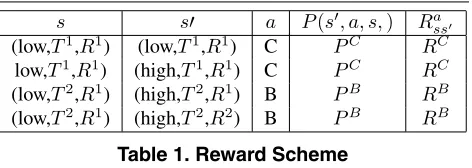
There are a total of 8 (2 Deadlines×2 Reservation Prices ×2 states of Resource Availability) states and 64 state tran-sitions for each action a. There is an estimation function

P(s, a, s,)and a reward functionRass associated with

ev-ery state transition and action. We have specified estimation probabilities and the reward scheme for a few such transi-tions in table 1. In a similar fashion they can be described for all the remaining state transitions.

s s a P(s, a, s,) Ra

ss

(low,T1,R1) (low,T1,R1) C PC _RC

low,T1,R1) (high,T1,R1) C PC _RC

(low,T2,R1) (high,T2,R1) B PB _RB

(low,T2,R1) (high,T2,R2) B PB _RB

Table 1. Reward Scheme

4.3. Results

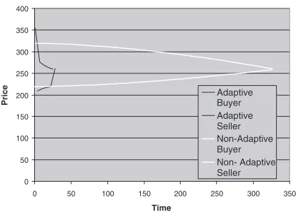
Having detailed the model’s instantiation, we now consider its effectiveness. To do this, for a specific set of negotia-tion parameters (Ta,RPa,IPa) we allowed a buyer and a seller to negotiate and measured the value at which an agreement was reached and the time taken to get there. In particular, we consider negotiation in the face of varying resource availability, two differentRP sand two different T s (since, as outlined in section 1, these two factors are the key drivers in e-commerce settings). Using the adaptive algorithm, the agent, at each state of the negotiation pro-cess, autonomously determines the optimal action (the one that yields the maximum future reward). This translates into choosing the parameter,ψ, that governs the offer,p, that the agent makes.

0 50 100 150 200 250 300 350 400

0 50 100 150 200 250 300 350

Time

Price

Adaptive Buyer Adaptive Seller Non-Adaptive Buyer Non- Adaptive Seller

Figure 1. Adaptive vs. Non-Adaptive Strategy

given in table 3. As can be seen, the value of the agree-ment is about the same in both the adaptive and the non-adaptive cases. This is because while specifying the re-ward scheme we have assumed that it is more important to reach an agreement before the deadline than the ac-tual value at which the deadline is reached (this could easily be changed to give more importance to the ac-tual outcome attained simply by specifying an alternate re-ward scheme).

Agent Buyer Seller

Initial Price 100 500 Reservation Price 300 or 250 250 or 200

Deadline 600 500

Table 2. Negotiation Parameters

Strategy Adaptive Non-Adaptive Time of Agreement 29 327 Value of Agreement 260 260

Table 3. Comparison Results

5. Conclusions and Future Work

In this paper we have developed a model for adaptive bi-lateral negotiation that is suitable for dynamic e-commerce environments. Specifically, we have used a non-stationary value iteration algorithm to determine non-stationary nego-tiation strategies when the dynamics of the system are only probabilistically known. This negotiation model can adapt the agent’s strategy in response to resources availability and variation in negotiation parameters (deadlines and reserva-tion prices). We believe that this represents an important step forward in the field of bilateral negotiations in that our mechanism gives the agents a method by which they can ne-gotiate effectively in a variety of situations in which the dy-namics of the system are not completely known. In partic-ular, this helps the agent to function in dynamic environ-ments, where it is impossible to know at the start of the ne-gotiations all the states that the agent might encounter. We have illustrated this approach by solving a representative negotiation problem. Initial results show that the time taken to reach an agreement can be significantly reduced com-pared to a non-adaptive strategy.

In future work we will extend the algorithm to deal with situations in which there is complete ignorance about the system dynamics (as opposed to the present probabilistic assumption) where the agent learns an optimal policy by re-peatedly negotiating with its opponent. We will extend the algorithm to cover the convergence aspects of our learning algorithm and will evaluate its suitability and effectiveness for online learning.

6. Acknowledgement

The work reported in this paper has formed part of the PDE area of the Core 3 Research Programme of the Vir-tual Centre of Excellence in Mobile & Personal Communi-cations, Mobile VCE, www.mobilevce.com, whose funding support, including that of EPSRC, is gratefully acknowl-edged. Fully detailed technical reports on this research are available to Industrial Members of Mobile VCE.

References

[1] A.Rubinstein. Perfect bargaining in a bargaining model.

Econometrica,50:97–110, 1982.

[2] F.Garcia and S.M.Ndiaye. A learning rate analysis of rein-forcement learning algorithms in finite horizon. Proceedings of the 15th International Conference on Machine Learning (ML-98), 1998.

[4] M.He, N.R.Jennings, and H.Leung. On agent-mediated elec-tronic commerce. IEEE Trans on Knowledge and Data Engi-neering, 15(4): 985-1003, 2003.

[5] M.L.Littman. Markov games as a framework for multi-agent reinforcement learning.Proceedings of the 11th International Conference on Machine Learning (ML-94), 1994.

[6] N.R.Jennings, P.Faratin, A.Lomuscio, S.Parsons, C.Sierra, and M.Woolridge. Automated negotiation:prospects, meth-ods and challenges.International Journal of Group Decision and Negotiation, 10(2): 199-215, 2001.

[7] P.Faratin, C.Sierra, and N.R Jennings. Negotiation decision functions for autonomous agents. International Journal for Robotics and Autonomous Systems, 1998.

[8] R.A.Howard.Dynamic Programming and Markov Processes. The MIT Press, 1960.