Classifier Systems Can Reduce
Conceptual Design Cycle Time
Andr´
as S´
obester
∗, Andy J. Keane
†University of Southampton, Southampton, Hampshire, SO17 1BJ, UK
Though very widely used in preliminary and detail design, commercial parametric CAD engines have not reached their full potential yet at the con-ceptual stage of industrial design processes. One possible reason is their lack of robustness when it comes to generating a wide variety of geome-tries, as demanded by the global nature of conceptual design. Such large, multi-dimensional design spaces often have regions of infeasibility, where the corresponding CAD models would lead to failure as early as the geometry generation process itself or as late as the final stages of some expensive mul-tidisciplinary analysis process integrated into the concept design tool. In this paper we discuss the use of Radial Basis Function classifier systems as a means of mapping out infeasible regions of the design space. The ultimate aim is to equip the concept design tool with the ability to avoid such areas, thus saving time by reducing the number of failed simulations on unphysical or otherwise unsuitable candidate designs.
Nomenclature
x vector of design variables
xi ith element ofx x(j) jth design vector
k number of design variables
N number of training designs
y N-vector of responses
y(i) label of designx(i)
φ(.) basis function ˆ
y feasibility prediction
wi coefficient of the ithbasis function w vector of basis function coefficients
σ hyperparameter of the Gaussian RBF
r distance of current point from the RBF centre
Φ matrix of basis function values / correlation matrix
∗Research Fellow, Computational Engineering and Design Group.
†Professor of Computational Engineering, Chair of Computational Engineering and Design Group.
I. Introduction
T
HE design of a new aircraft is often viewed as a three-phase process. The conceptual design phase translates the customer’s needs and the relevant airworthiness requirements into an ini-tial, baseline design.1 The level of detail increases throughout thepreliminary phase, while thedetail design stage produces the blueprints of the individual parts and the plans of the corresponding man-ufacturing processes. There isn’t a clear consensus between the established textbooks as to where exactly the dividing lines between the three phases lie on this continuum of increasing design detail and analysis fidelity (compare, for example, the taxonomies of Torenbeek1and Raymer2) – in this work we attach the label ‘conceptual’ to design of the minimum level of detail necessary for a meaningful multidisciplinary study of the trade-offs involved in arriving at a baseline airframe.The conceptual design process is, essentially, a highly global search over the space of possible con-figurations, shapes and dimensions. The solution chosen to progress to the preliminary design stage is usually one that satisfies all the constraints and optimizes some figure of merit, related to perfor-mance,3–5 cost,6 revenue or combinations of these.7–11 To compute these metrics and make design decisions based on them, the design system needs to integrate the various strands of multidisciplinary analysis into an iterative process, often driven by an optimization engine. The reader interested in the precise nature of the workflow within such systems may consult the detailed descriptions of vari-ous MDO (Multidisciplinary Optimization) frameworks (see, e.g., Sobieski’s BLISS12) or some of the relevant surveys.13, 14 Here we focus on what should, in the age of modern, mature CAD systems, lie at the heart of any such process: the geometry engine, supplying the models required by the various numerical simulation codes that make up the multidisciplinary analysis capability of the system (for an example of such a CAD-centered system see the reports on the MOB project, e.g., La Rocca et al.15 and ¨Osterheld et al.16).
Arguably, the global nature of the conceptual design process requires a CAD model that encom-passes a broad range of possible designs. In an ideal world a seamless parameterisation would be required, which ensures that the optimizer can visit a wide variety of configurations and can move between them smoothly, as driven by the objective function. In reality, however, the uniform, flawless coverage of the design space by a generic CAD model is fraught with difficulties∗. In all but the most
trivial or overconstrained cases the construction of the geometrical model can fail in certain areas of the design space. Of course, if these areas are rectangular, they can simply be avoided by adjusting the bound constraints on the relevant variables, but this is rarely the case. Most of the time the infeasible areas will have complex, irregular shapes and are much harder to identify and avoid. The problem therefore usually boils down to the following trade-off. One can place bound constraints on the design variables that are sufficiently tight so as to ensure that any possible combination of variables will lead to a feasible design – the drawback here is that the design space will be very limited. Alternatively, wide bound constraints can be used to enable the exploration of a wide variety of designs, with the risk that the model generation process will fail occasionally.
In the present work we advocate the use of RBF (Radial Basis Function) network classifiers to alleviate the problems related to the latter situation. We see RBF classifiers fulfilling a dual role in
∗Parameterisation technology has come a long way since the first tentative numerical design optimisation efforts of
the 1970s (see, e.g., Samareh’s recent survey17
of developments in this field). As a result, techniques are available today for robust parameterisation of relatively simple subsystems (such as aerofoils) – nevertheless, the reliableand flexible parameterisation of complete aircraft models is still a considerable challenge.
the design process. First, the classifier model can be used to filter out infeasible geometries before they are generated. This can contribute to the reduction of design cycle time by avoiding expensive, pointless computations performed on bad geometries. In a conventional automated MDO system such designs may be highlighted by the failure of the CAD tool to generate a meaningful model (e.g., when a feature is defined by the intersection of entities that no longer intersect), in which case “only” a few minutes are lost. However, if the shape is geometrically meaningful, but merely unphysical (e.g., wildly snaking splines in a wing section), alarm bells only start ringing when, say, the aerodynamic flow simulation fails to converge even after a large number of iterations – by which time hours of CPU time may have been wasted.
A possible secondary role for an RBF classifier (which we will only touch on briefly here) could be to aid in the construction of feasible designs, given certain fixed parameters. For example, the designer may want to define the outline of the center section of a blended wing-body airframe as well as the desired wing sections and use the RBF model to suggest feasible centre body-wing fillet regions. In the next section we discuss the technical aspects of constructing such classifier models – this will be followed by an application of the technique in Section III. Section IV. contains our conclusions and outlines possible extensions to the scheme described here.
II. Building a Radial Basis Function Classifier
Let us consider a set ofN design vectors (each taking the formx(i)= (x1, x2, ..., xk)), denoted by
[x(1),x(2), . . . ,x(N)], which we will use to train our classifier. We assume that each component within this vector can be labeled as feasible or infeasible (1 or -1 respectively) and we define the response vector y = [y(1), y(2), . . . , y(N)] containing these labels. Radial basis functions can be used to make a prediction ˆy = ˆf(x) at any point xin the design space. We use N bases and we center the basis functions around the N labeled points (i.e., [x(1),x(2), . . . ,x(N)]). The basis functions take the form
φ(kx−x(i)k), whereφ(·) is some (usually) non-linear function, theithsuch function depending on the
Euclidean distance betweenxandx(i). The predictor is a linear combination of these basis functions, that is,
ˆ
y= ˆf(x) =
N X
i=1
wiφ(kx−x(i)k). (1)
Defining the vectorw= [w1, w2, . . . , wN]T and the matrixΦi,j =φ(kx(i)−x(j)k), wherei= 1, . . . , N, j = 1, . . . , N and introducing a ridge regression† parameterλ, the coefficients can be determined by
solving (Φ+λI)w=yT (provided, of course, that the inverse ofΦ+λIexists): w= (Φ+λI)−1yT.
A prediction ˆy can now be made in any pointx(N+1)∈D by computing ˆy(N+1)=φw,where
φ=hφkx(N+1)−x(1)k, φkx(N+1)−x(2)k, . . . , φkx(N+1)−x(N)ki. (2) Many different basis functions φ(·) could be considered. Throughout this work we have used exponentially decaying positive definite Gaussian basis functions φ(r) = exp(−r2/2σ2). (1) is thus a parametric model and the correct estimation of the hyperparameterσ, which governs the regions of influence of each kernel, is important and can affect prediction accuracy. In the work presented here we use a generalised version of the leave-one-out cross validation procedure. The leave-one-out
†We note here that an interpolating RBF (i.e.,λ= 0), although a perfect classifier of the training data, would, of
course, generalise very poorly.
measure is an almost unbiased estimator of the empirical risk, which, in turn, is an estimate of the generalisation error of the model (the true risk).14 In practical terms, the leave-one-out estimator can be computed as follows. For each value of σ under consideration we build N RBF models leaving out one of the training points in each case (as though we only had N−1 points), we compute the difference between the true objective value of the currently left out point and the objective predicted by the partial model (which uses the remaining N−1 points) at the same point. The final model is constructed using the value ofσ that minimizes the sum of the squares of these residuals. The same applies to the computation of the optimum regression parameterλ(the training process is therefore a two-variable optimization problem).
We note here that special care is required if the training set is large. In such cases the variance of the leave-one-out estimator can be high (due to the subsets created by leaving out a point being very similar), so it may be preferable to use a leave-q-out crossvalidation estimator, which is biased, but has a lower variance.14 The computational cost of model training based on this generalised measure is also lower (forq >1)‡.
Practical Considerations
An effective case-based reasoning system (as this is what the method discussed here essentially amounts to) has to be able to incorporate both explicit and implicit rules. For example, given two design variablesx1and x2, we may not want to restrict their ranges, but we may want to make sure that, say,x1is always less thanx2. This is an explicit rule. An implicit rule may be a similar law, but one that we cannot discover simply by using engineering (or geometrical) judgement and therefore it is left to the system to detect any such relationships based on the training data.
The RBF classifier system described above is capable of handling both. The training data can be labeled in two stages. First, training points that break any of the explicit rules will be labeled with -1. The labels of the remaining designs (i.e., CAD geometries) will be determined by visual inspection – each of these models has to be built using the interactive mode of the CAD engine and labeled accordingly.
Another practical issue is that of the interpretation of the model. We mentioned in Section I. that our goal here is two-fold. First, we want to be able to filter out designs that are likely to fail. Secondly, we may want to construct feasible designs based on fixed values of some of the parameters. The filtering role of the classifier raises the issue of balancing model reliability versus search space size. If our design search DoE (Design of Experiments) contains a pointxfor which the predictor ˆy(x) exceeds a certain threshold value t, we go ahead with the multidisciplinary analysis of that design and if ˆy(x)< t, we discard it as a design that is likely to fail (either at the CAD model building or at the analysis stage). The reliability versus globality question arises when choosing t – the larger its value, the more certain we can be that the designs exceeding it will be feasible, but, of course, the added confidence will carry a search space reduction penalty. We shall use the example in the following section to provide further guidance on how this parameter can be chosen.
As far as the second goal, the construction of feasible designs, is concerned, the situation is more straightforward: we simply maximize the predictor (1), subject to the equality (or even inequality)
‡This is sometimes referred to asq-fold crossvalidation – in that caseqrefers to the number of subsets the training
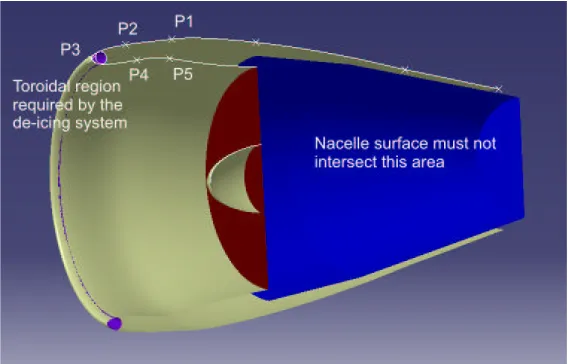
Fig. 1 Longitudinal section through the CATIA model of the jet engine nacelle.
H1 V1 H2 V2 H3 V3 H4 V4 H5 V5
Lower bound 0.25 0.59 0.4 0.5 0.6 0.45 0.4 0.45 0.1 0.45 Upper bound 0.5 0.63 0.8 0.62 1.0 0.62 0.8 0.55 0.5 0.55
Table 1 Bound constraints on the design variables describing the nacelle geometry.
constraints determined by the designer’s requirements. In other words, the design likely to be the most feasible can be found by maximizing the predictor with the relevant variables fixed or the search space restricted in the relevant dimensions.
We now proceed to illustrate the algorithm described above by means of an example – the design of a jet engine nacelle.
III. An Application – Design of a Jet Engine Nacelle
The CATIAR
model of the geometry we propose to examine here is shown in Figure 1. We focus on the handling of the geometry of the lip, defined by 5 points (P1 through P5), each having two degrees of freedom, i.e., being allowed to move in the symmetry plane. The surface of the lip is a surface of revolution, whose generator is a spline going through the five control points and three fixed nodes defining the aft part of the cowl, being additionally constrained by having to be normal to the fan face.
Table 1 contains the bounds placed on the design variables. Hi andVi denote the horizontal and
vertical coordinates of control point Pi, measured in an axis system with its origin in the fan face
centre and the H axis pointing upstream and the V axis pointing upwards. Additionally, the following explicit rules have been defined: H5+ 0.075< H4,H1+ 0.075< H2,V1> V5+ 0.06,V2> V4+ 0.06 and max{H2, H4}+ 0.03< H3.
The geometry can fail by violating any of the following constraints. First, we assume that the dark area behind the fan face is the external envelope of the bypass air duct and therefore must not be intersected by the nacelle surface. The second constraint relates to de-icing requirements: we define a toroidal region, whose radius is equal to the optimum impingement distance of the piccolo tube, which has to fit inside the leading edge of the lip (the CAD model automatically finds the location
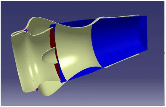
[image:5.612.164.448.104.286.2]Fig. 2 Longitudinal section through a typical failed nacelle model.
for this torus nearest to the leading edge). This must not be intersected by the nacelle surface and the centre of its generator circle must not be more than 1.3 radii away from the inside of the surface. In other words, sharp leading edges must be avoided. Further, while “bumps” in the internal and external surfaces of the nacelle are allowed, excessive snaking and sharp transitions are not. Figure 2 illustrates all three of these modes of failure.
For the purposes of training the model, 1,000 points have been generated in a 10-dimensional Morris-optimal latin hypercube experimental design. In the first stage of the training process the explicit rules have been applied – this lead to 718 points receiving the -1 label. Next, the CAD model was run for the remaining 282 points, all of which have been examined and labeled according to the three failure criteria mentioned earlier (22 receiving the -1 label, 260 the +1 label). An RBF model was fitted to this data, trained using the leave-q-out criterion (with q = 25). The resulting model was then used to “predict back” the training data – the histograms in Figure 3 depict the results. The histogram on the left hand side of the figure represents the values of the predictor for the failed training points (i.e., those that we have labeled -1 in the training process), while the histogram on the right depicts the predictions for the models known to be “healthy”. To get an assessment of the generalisation properties of the classifier, we have generated and classified another set of 100 points (again, arranged in a Morris-optimal latin hypercube experimental design) – the values of the predictor in these points are depicted in Figure 4 on a histogram similar to that discussed above.
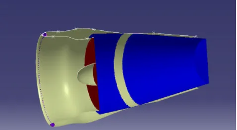
An important aspect of these plots from the threshold (t) selection point of view is that the two histograms overlap slightly. Clearly, we can safely reject any design with a feasibility indicator below -0.5 and we can safely accept any design with ˆy > 0.15. Therefore, t must lie between these two values, with the willingness of the designer to accept the occasional failed run for the sake of keeping the design space as large as possible deciding on the actual value. We note here that the overlap area is likely to contain the borderline cases, i.e., those designs where, for example, the nacelle does not intersect the restricted area reserved for the turbine, but is tangent to it (see Figure 5).
[image:6.612.163.450.103.288.2]−1.50 −1 −0.5 0 0.5 1 1.5 50
100 150 200 250 300
Feasibility indicator (RBF)
Number of training designs
Unfeasible designs in the training data
Feasible designs in the training data
Fig. 3 Distributions of the 1,000 failed and feasible training designs, according to their feasi-bility indicators (RBF predictor values).
−1.50 −1 −0.5 0 0.5 1
5 10 15 20 25
Feasibility indicator (RBF)
Number of test designs
Unfeasible designs in the test data Feasible designs in the test data
Fig. 4 Distributions of the 100 failed and feasible test designs, according to their feasibility indicators (RBF predictor values).
Fig. 5 Example of a borderline design from the area where the two histograms (feasible and failed) overlap. The design would be classified as ‘failed’ due to the slight contact between the nacelle surface and the fan casing. The value of the RBF predictor is -0.51.
IV. Conclusions and Implications
In this paper we have advocated the use of Radial Basis Function classifier systems as a means of capturing some of the designer’s knowledge of which geometries are likely to be infeasible as design candidates. This knowledge can then be deployed in an automated design system, where it can reduce the number of infeasible designs fed into the multidisciplinary analysis module(s). Clearly, no classifier can give a definitive prediction of the feasibility of design, but it can achieve the main goal of reducing the number of failures in the optimization cycle and thus reduce conceptual design cycle time.
[image:7.612.147.469.111.218.2] [image:7.612.148.466.269.379.2] [image:7.612.187.426.426.557.2]Like most global predictors, RBF networks are affected by the “curse of dimensionality”, that is, they need exponentially increasing amounts of training data as the number of design variables increases. Therefore, large models, with tens or hundreds of variables, must be broken down into sub-models (perhaps with overlapping sets of variables), which are predictable with a reasonable number of training cases. The essential step here is to identify the subsets of design variables, which have an influence over any particular failure mode of the geometry.
An additional advantage of such classifiers is the relative ease of their implementation and mainte-nance. Once incorporated into a conceptual design tool, the classifier can expand its training database each time a new model is built and analysed – computer idle time can be used to occasionally retrain the predictor.
Throughout this paper we have devoted a lot of attention to the idea of identifying infeasible designs before they waste precious computing time, but we have not discussed in great detail its possible implications from the perspective of the optimization process. This is the subject of future work and a number of possible avenues can be explored.
The simplest strategy is, of course, to simply discard designs that are deemed infeasible – many standard optimization algorithms can be modified to cope with failures in this way. However, this approach may not allow us to explore the feasibility boundary, which may be the location of many good designs. A better alternative is to repair the failed designs, that is, to find the feasible design nearest to them. This is, essentially, a different way of looking at the feasible geometry construction role mentioned earlier – it can thus be done using the classifier itself, by locally optimizing it in the basin of attraction of the failed design.
Acknowledgements
This work has been jointly supported by BAE Systems and the Engineering and Physical Sciences Research Council.
References
1
Torenbeek, E.,Synthesis of Subsonic Airplane Design, Kluwer Academic Publishers, Dordrecht, 1982.
2
Raymer, D. P.,Aircraft Design: a Conceptual Approach, AIAA Education Series, American Institute of Aero-nautics and AstroAero-nautics, Washington DC, 3rd ed., 1999.
3
Jameson, A., “Re-engineering the Design Process Through Computation,”Journal of Aircraft, Vol. 36, No. 1, 1999, pp. 36–50.
4
Baker, C. A., Grossman, B., Haftka, R. T., Mason, W. H., and Watson, L. T., “High-Speed Civil Transport Design Space Exploration Using Aerodynamic Response Surface Approximations,”Journal of Aircraft, Vol. 39, No. 2, 2002, pp. 215–220.
5
Butler, R., Hansson, E., Lillico, M., and Van Dalen, F., “Comparison of Multidisciplinary Design Optimization Codes for Conceptual and Preliminary Wing Design,”Journal of Aircraft, Vol. 36, No. 6, 1999.
6
Scanlan, J., Hill, T., Marsh, R., Bru, C., Dunkley, M., and Cleevely, P., “Cost Modelling for Aircraft Design Optimization,”Journal of Engineering Design, Vol. 13, No. 3, 2002, pp. 261–269.
7
Markish, J. and Willcox, K., “Value-Based Multidisciplinary Techniques for Commercial Aircraft System Design,”
AIAA Journal, Vol. 41, No. 10, 2003, pp. 2004–2012.
8
Willcox, K. and Wakayama, S., “Simultaneous Optimization of a Multiple-Aircraft Family,”Journal of Aircraft, Vol. 40, No. 4, 2003, pp. 616–622.
9
Collopy, P. and Horton, R., “Value Modeling for Technology Evaluation,”38th AIAA/ASME/SAE/ASEE Joint
Propulsion Conference and Exhibit, Indianapolis, Indiana, July 7-10, 2002.
10
Peoples, R. and Willcox, K., “A Value-Based MDO Approach to Assess Business Risk for Commercial Aircraft Design,”10th AIAA/ISSMO Multidisciplinary Analysis and Optimization Conference, Albany, 2004.
11
Antoine, N., Kroo, I., Willcox, K., and Barter, G., “A Framework for Aircraft Conceptual Design and Environ-mental Performance Studies,” 10th AIAA/ISSMO Multidisciplinary Analysis and Optimization Conference, Albany, 2004.
12
Sobieszczanski-Sobieski, J., Altus, T. D., Phillips, M., and Sandusky, R., “Bilevel Integrated System Synthesis for Concurrent and Distributed Processing,”AIAA Journal, Vol. 41, No. 10, 2003, pp. 1996–2003.
13
Perez, R. E., Liu, H. H. T., and Behdinan, K., “Evaluation of Multidisciplinary Optimization Approaches for Aircraft Conceptual Design,” 10th AIAA/ISSMO Multidisciplinary Analysis and Optimization Conference, Albany, 2004.
14
Keane, A. J. and Nair, P. B.,Computational Approaches to Aerospace Design: the pursuit of excellence, John Wiley & Sons., 2005.
15
La Rocca, G., Krakers, L., and van Tooren, M. J. L., “Development of an ICAD Generative Model for Blended Wing Body Aircraft Design,”9th AIAA/ISSMO Symposium on Multidisciplinary Analysis and Optimisation, Atlanta, 2002.
16
Osterheld, C., Heinze, W., and Horst, P., “Preliminary Design of a Blended Wing Body Configuration using the Design Tool PrADO,”CEAS Conference on Multidisciplinary Aircraft Design and Optimisation, Koln, 2001.
17
Samareh, J. A., “Survey of Shape Parameterization Techniques for High-Fidelity Multidisciplinary Shape Opti-mization,”AIAA Journal, Vol. 39, No. 5, 2001, pp. 877–883.