Material Cost Prediction for Jewelry Production Using Deep Learning Technique

Article

Material Cost Prediction for Jewelry Production Using

Deep Learning Technique

Chanida Phitthayanon

_{and Vichai Rungreunganun}

Department of Industrial Engineering, Faculty of Engineering, King Mongkut’s University of Technology North Bangkok, Bangkok, Thailand

E-mail: a _{ajchanidap@hotmail.com,} b_{r_vichai@yahoo.com (Corresponding author)}

Abstract. Production cost management is a key factor to increase industrial competitiveness.

The precious metals and the gemstones comprise 65% of the jewelry material cost. Managing raw material cost is a challenging task especially when the price highly fluctuates. In this article, deep learning models were proposed to predict the prices of main raw materials of jewelry which are silver, gold, and diamond. These models are designed for Thai jewelry manufactures which are mostly small businesses. Therefore, our models only consider historical price data. This is because small businesses usually do not have access to other relevant data, i.e. oil prices and other economic data.

The proposed precious metal price model can provide prediction with RMSE of 0.00765 which is comparable to other models in literature while requires less data and offers a simpler model. Also, the proposed diamond price model can provide RMSE of 0.0181 which is 42.41% improvement from the model normally used by jewelry manufacturers.

In addition to the raw material price prediction model, a quantization method of diamond 4C grade is proposed and validated statistically and visually. This quantization method could be used in a diamond analysis.

Keywords: Jewelry, deep learning, diamond price, silver price, gold price.

ENGINEERING JOURNAL Volume 23 Issue 6

1.

Introduction

The gems and jewelry industry is a large part of Thailand economic with the export value of more than USD 11.900 billion [1] which is the third most valued export product. The industry employed more than 800,000 jobs [2]. It is reported that gemstone cost and precious metal cost take a large part in the jewelry cost structure [3], which is approximately 35% and 30% of the production cost, respectively. Thai jewelry manufacturers are mostly small and medium businesses (SMEs) [2]. There were more than 15,000 businesses in the industry with 64.4 % of them are small family businesses and 31.1 % of them are medium businesses.

For them to manage risks of fluctuations in gemstone and precious metal prices, they usually rely on the naive price forecast method. For example, the naive forecasting method would assume the last month price of the gemstone will occur again this month or assuming a fix percentage increase in the price. These naive forecasting assumptions are easy and widely used by jewelry SMEs. On the other hand, statistical price forecasting models are a fitted curve through historical demand quantities with a seasonality, trend data, and a moving average value. These statistical forecastings are more difficult and time consuming for jewelry SMEs.

A study of Thailand gems and jewelry industry [4] found that jewelry manufacturers suffer from the fluctuation of raw material prices. This price fluctuation imposes more impact on the jewelry industry during 2006 and 2014, when gold and silver prices were changed rapidly [5], [6]. It is indicated in a study of factors influencing the competitiveness of jewelry industry that price forecasting ability is the third-highest impact factor [7].

On the contrary, the investors in the future exchange market generally use traditional time-series forecasting models that can be customized and fine-tuned, such models are too complicated and too much time consuming to be used by small and medium businesses. Machine learning forecasting models have gained a lot of attention. Recently, machine learning models can give a better prediction result than time-series approaches. Another big advantage of using a machine learning model is that after the initial development, SMEs users need minimal training and take small time using the model to forecast material prices.

In this work, recent literature related to diamond, gold, and silver price forecasting is reviewed in Section 2. Then, the machine learning methodologies used in this work are shown in Section 3. The proposed deep learning models are discussed in Section 4 and 5 for the precious metal price and diamond price models, respectively. And followed by, the conclusion in Section 6.

2.

Literature Review

Several studies of precious metal and diamond prices have been done using various statistical models. For instance, in 1992, von Saldern purposed a non-linear optimization model to forecasting rough diamond prices [8]. In 1996, a simple linear regression was done to study diamond ring prices [9]. In 2013, an analysis of the diamond price was carried out using an unconditional quantile regression model [10]. Another analysis of diamond as an asset in the global market was performed [11]. In this work, a short/long term investment of diamond for various grades was studied. In 2015, a price-quality dispersion analysis was performed for the online diamond market [12].

In 2008, Mongkolkaset surveyed of factors affecting gold price [13]. The result shows that the factors affecting the gold price are all global factors, i.e. the global national income (GNI), the global consumer price index, the nominal currency exchange rate, etc. These factors are difficult to collect and estimate for small businesses.

Therefore, other research groups have proposed various models to predict the gold price based on the historical price only without relying on any external data. These works utilize time-series analysis techniques. For example, in 2013, Keerativibool reported another study of a gold ornament selling price using Holt’s exponential smoothing method [14]. In 2016, Bandyopadhyay proposed a forecasting method for the gold price using the ARIMA model [15]. And, Shafiee has summarized the global gold market and gold price forecasting [16]. Another statistical model was proposed for the daily gold price [17].

While these statistical techniques have been widely studied and used in industrial, new modern techniques such as time-series forecasting with machine learning that is based on supervised learning method have limited used in jewelry manufacturers [23]. In 2004, a gold price predicting model was proposed using simple feed-forward neural network models with genetic algorithms [24] using NYMEX daily gold price. The gold and silver price prediction have been well studied in the literature with only a small room of improvement.

On the other hand, the diamond price prediction in the literature is limited. In part, it is because the diamond market has been driven by the upstream global diamond supplier, i.e. De Beer Group. The company issues its annual report about the diamond industry [25] in which include the diamond price trends. However, the diamond price used by the jewelry industry relies on Rapaport’s Rapnet [26] and IDEX [27]. The lack of diamond price prediction in the literature is a big research gap.

3.

Methodology

In this section, the data science methodologies used in this work are outlined. The methodology steps are: - Collect data from a credible source

- Clean data from missing data - Transform and normalize data - Create a model

- Training and verify the model

- Validate model and improve the model (if needed)

3.1. Data Source, Cleaning, and Transformation

3.1.1. Gold and silver price data

The gold and silver metals are considered as commodity products and they are traded in many commodity markets. Gold and silver metals are traded in both types of commodity markets, i.e. physical trading and derivative trading. In physical trading, an actual product will be delivered to the buyer. While, in the derivative trading, no actual product will be delivered to the buyer. In both types of trade, there are many prices as well. A spot contract is a buying or selling for immediate settlement on the spot or within two business days after the trade date. This settlement price is called the spot price. On the other hand, a forward contract is a non-standard contract for buying or selling at a specific future time at a price agreed upon today. Similarly, a future contract is a standardized forward contract where buying or selling at an agreed price at a specific time in the future. Lastly, an option contract is a contract in which the buyer has the right, but not the obligation, to buy at a specific price before or on a specific future date.

Jewelry manufacturers need the actual product to be delivered which is the physical trading. There are many gold and silver local markets in countries around the world. For example, New York, London, Hong Kong, and Sydney are globally recognized markets [28] in which the price data is achieved and analyzed. However, jewelry manufactures mostly do not locate in these regions. So, they must rely on their local market price in which the price data may not be properly archived and unavailable for analysis. However, these local market prices usually rely on global commodity trading price, i.e. London Fixed. And, the price change in the global market will quickly affect the price in local markets. Therefore, this work uses the spot price data of gold and silver metal in our analysis.

In this work, the historical gold and silver price data was obtained from Gold Spot US Dollar (XAUUSD) and Silver Spot US Dollar (XAGUSD) at London Fixed market. The price data which were collected daily at 3.00 PM. The gold and silver price data were collected and archived by usagold.com and available at [5], [6], respectively.

The gold and silver price data are on the daily period from January 3th, 2000 to October 31st, 2018, except weekends and holidays. Although there are 6,876 calendar days in this period, the price data is only available for 4,772 days. This is because the trading price is not available on holidays and weekends. Therefore, we cleaned the missing data by ignoring the date, because the trading markets are closed on these missing dates. Hence, the price data consists of 4,772 time-steps (days).

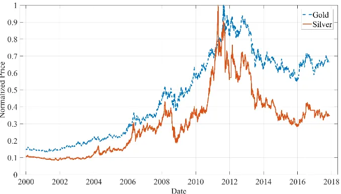
Fig. 1. Normalized price of gold and silver metals. The gold and silver spot price data are normalized to their maximum values of 1,908.82 USD per ounce on 21-Aug-2011 and 48.283 USD per Ounce on 27-Apr-2011 for the gold and silver metals, respectively.

3.1.2. Diamond price data

Unlike gold and silver, diamond is not a commodity product. Each diamond is unique and its price vary widely based on the quality of the individual diamond. The quality of a diamond can be graded using 4C grade [29]. These 4C grades are color, clarity, cut, and carat. The color quality is evaluated based on the absence of color with the grade value range from D to Z. The D grade representing colorless and increasing with color to the Z grade. The clarity quality refers to the absence of inclusion and blemishes with the grade value range from FL to I3. The cut quality is the ability of diamond’s facets interact with light with the grade value range from excellent to poor. And, the carat-sizes measures the diamond size by its weight. The weight of 1 carat is defined as 0.2 gram.

The global diamond market often refers to the Rapaport price list as the benchmark price [26]. The Rapaport price data contains 3,400 variations of the diamond 4C grade. The Rapaport data includes 10 color grades range from D to M, 11 clarity grades range from IF to I3, 2 cut shapes (pear and round), and 20 carat-sizes range from 0.01 to 10 carats. The Rapaport price list is not the price of an individual diamond, but it is the price of diamond amount 1-carat weight of a specific grade. For example, The Rapaport price list indicated that a diamond of 0.2 carats, D color, IF clarity, and round shape was price at 65 hundred USD per carat in July 2011. This means that an individual diamond of the same grade could be sold with an asking price of 1,300 USD cash. Another example, for the diamond of 5 carats, D color, IF clarity, and round shape was price at 1018 hundred USD per carat in June 2008. So, an individual diamond of the same 4C grade could be valued as 509,000 USD cash.

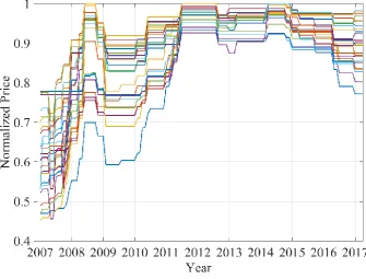
Fig. 2. Normalized price of some diamond grades.

Next, the histogram of the number of times that the diamond price was changed is as shown in Fig. 3. The diamond price is quite steady because the diamond prices had been changed only 8.34 times on averagely, over the 124 time-step. There were 76 diamond grades that their price had never been changed over the 10 years. There were about 300 diamond grades that their price had been changed only 3 times. And, prices of the diamond grade with the most fluctuate price had been changed only 30 times.

Fig. 3. Histogram of diamond price change over 10 years.

3.1.3. Transforming diamond 4C features

For the cut grade, the Rapaport price list only provides a diamond price for the pear shape and the round shape with brilliant-cut quality. Therefore, the cut feature can be represented using 1-hot encoding in which the 𝐼𝑠𝑅𝑜𝑢𝑛𝑑 and 𝐼𝑠𝑃𝑒𝑎𝑟 features represent the round shape and pear shape, respectively.

For the clarity and color quality grades, these two features are not categorical data because, for both clarity and color grades, a diamond with a higher the grade will have a higher the price. Therefore, these two features can be transformed into discrete data. Therefore, the quantified 4C features represented in numeric forms are shown in Table 1.

Table 1. Quantization of diamond cut, clarity, and color grades.

IsRound IsPear Clarity Color

Cut Value Cut Value Grade Value Grade Value

Pear 0 Pear 1 I3 1 M 1 Round 1 Round 0 I2 2 L 2 I1 3 K 3 SI3 4 J 4 SI2 5 I 5 SI1 6 H 6 VS2 7 G 7 VS1 8 F 8 VVS2 9 E 9 VVS1 10 D 10

IF 11

Next, a validation of our quantization of diamond 4C grades were performed by a multiple linear regression on the diamond price data with the quantified 4C features. Since there are both positive and negative trends on the price, we reduced the trends in the data by using natural logarithm of the prices. The linear model is:

ln 𝑃𝑟𝑖𝑐𝑒 = 𝛽0+ 𝛽1𝐼𝑠𝑅𝑜𝑢𝑛𝑑 + 𝛽2𝐼𝑠𝑃𝑒𝑎𝑟 + 𝛽3𝐶𝑙𝑎𝑟𝑖𝑡𝑦 + 𝛽4𝐶𝑜𝑙𝑜𝑟 + 𝛽5𝐶𝑎𝑟𝑎𝑡 (1)

We perform linear regression analysis and the result is as follow. The fitted model has the adjusted R-square value of 0.657 and all coefficients are statistically significant. The coefficient estimates and their statistic values are shown in Table 2.

Table 2. Coefficient estimates and their statistic values.

Coeff. Estimate SE t-stat p-value

𝛽₀ 0 0 - -

𝛽1 1.1910 0.0039832 299.0 0

𝛽₂ 1.1179 0.0040258 277.7 0

𝛽₃ 0.17126 0.0003971 431.2 0

𝛽4 0.11750 0.0004334 271.1 0

𝛽₅ 0.33458 0.0004931 678.5 0

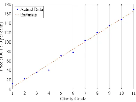
From the analyzed estimate shown in Table 2, we can see that a round cut diamond is about 6.5% more expensive than a pear cut diamond. A diamond with a level better in clarity grade is about 17% more expensive, as shown in Fig. 4. Similarly, a diamond with a level better in color grade is about 11% more expensive, as shown in Fig. 5. And, a diamond with a carat larger size is about 33% more expensive, as shown in Fig. 6.

Fig. 4. Relationship between the diamond price and its clarity feature. Clarity grades of I3 to IF are quantified as 1 to 11, respectively. The blue dots indicate the average price for each clarity grade.

Fig. 5. Relationship between the diamond price and its color feature. Color grades of M to D are quantified as 1 to 10, respectively. The blue dots indicate the average price for each color grade.

3.2. Machine Learning Model

After data collection, cleaning, and transformation, machine learning models were created, trained and verified. The price data of precious metals is highly fluctuating and in the daily period, while the price data of diamond is quite steady and in the monthly period. Because the two data is in a different format, the jewelry material cost model consists of two parts which are the precious metals part and diamond part. This approach is more beneficial to jewelry manufacturers because they usually manage inventories of precious metals and gemstones separately.

The machine learning models used in this work are naive forecasting model, decision tree-based models, and deep learning models.

3.2.1. Naive forecasting model

For time-series data, the naïve forecasting method is to forecast that all forecasted values are the same as the last observed value [31]. The forecasted value for time 𝑇 + ℎ is written as:

𝑦̂_𝑡+ℎ = 𝑦_𝑡−1 (2)

where 𝑦_𝑡 denotes data value at time 𝑡 and 𝑦̂ denotes a forecasted value. Despite its simplicity, this method works remarkably well for many common time-series data, especially for economic and financial domain [31].

3.2.2. Generalized linear model

A generalized linear model is an extension of Ordinary Least Square model (OLS) with the following formula:

𝑦𝑡 = ∑ 𝑤𝑗𝜙𝑗(𝑥𝑡) 𝑛

𝑗=0

(3)

where 𝑛 is the order of the model, 𝑤𝑗 is the weight of each term, and 𝜙𝑗( ) is the non-linear basis function.

The algorithm could fit the data by maximizing the log-likelihood. The non-linear basis function could be polynomial or gaussian function. The polynomial basis function is defined as 𝜙𝑗(𝑥) = 𝑥𝑗 for 𝑗 = 0,1,2, … , 𝑛

and the Gaussian basis function is defined as 𝜙_𝑗(𝑥) = (𝑥 − 𝜇𝑗)/(2𝜎𝑗2).

3.2.3. Decision tree

A decision tree is a topology of nodes that connect from the root node to the leaf. Each node represents a conditional evaluation of an attribute to create a decision on values of an estimate of a numerical target value. In this work, the target value is price data. Each node represents a splitting rule of an attribute. For regression or prediction problem, it separates them to minimize the estimation error.

3.2.4. Random forest

A random forest is a set of random trees which are built and trained on a subset of the data. The trees are combined to produce a final prediction. The validation and testing processes are performed using the forest.

3.2.5. Nonlinear autoregressive neural network with external inputs

The nonlinear autoregressive neural network with exogenous variables (NARX) is a feedforward network, with feedback connections from output layers of the network [32]. The NARX model is an extension from the linear autoregressive neural network with external inputs (ARX) model. The definition of the NARX model [33] is:

where the next-step value of the dependent variable 𝑦_𝑡 is regressed on the previous values of the dependent variable 𝑦_𝑡−𝑖 and the previous values of the exogenous variables 𝑢_𝑡−𝑖, where 𝑖 = 1, 2, … , 𝑛_𝑦 and 𝑖 = 1, 2, … , 𝑛𝑢 for the dependent variable and exogenous variables, respectively. We can implement the NARX

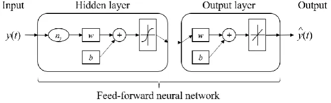
model using a feed-forward neural network to calculate the function 𝑓( ). The diagram of the NARX network is shown in Fig. 7.

Fig. 7. Diagram of a feed-forward neural network implementing the NARX model.

3.2.6. Nonlinear autoregressive neural network

The nonlinear autoregressive neural network (NAR) is a reduction model of the NARX model by removing the exogenous variable terms [34]. The definition of the NAR model [33] is:

𝑦𝑡 = 𝑓 (𝑦𝑡−1, 𝑦𝑡−2, … , 𝑦𝑡−𝑛𝑦) (5)

where the next-step value of the dependent variable 𝑦𝑡 is only regressed on the previous values of the

dependent variable 𝑦𝑡−𝑖, where 𝑖 = 1, 2, … , 𝑛𝑦. Similar to the NARX model, we can implement the NAR

model using a feed-forward neural network to calculate the function 𝑓( ). The diagram of the NAR network is shown in Fig. 8.

Fig. 8. Diagram of a feed-forward neural network implementing the NAR model.

3.3. Training and Verification of the Model

The training process of deep learning models was done using the standard Levenberg-Marquardt backpropagation optimization method [35], [36] which is an extension of the Newton method by adding an adaptive backpropagation with an initial step size of 0.001. The adaptive step size is increased or decreased to ensure the performance goal. The mathematic formula of the Levenberg-Marquardt algorithm [37] is as followed. The performance function is the sum of squares. The gradient can be calculated as 𝑔 = 𝐽𝑇_{𝑒, where}

and biases, and 𝑒 is the vector of the neural network errors. The Jacobian matrix can be computed using standard backpropagation technique [38]. Then, the weight of the neural network can be updated using

𝑥_𝑘+1= 𝑥_𝑘− [𝐽𝑇_{𝐽 + 𝜇𝐼]}−1_𝐽𝑇_{𝑒, where the scalar 𝜇 is adaptively change based on the performance value. The}

detailed algorithm of the LM training can be found in [37].

The split-sample method is used, i.e. splitting the data by 70% for training, 15% for validation, and 15% for testing. In data science methodology, a data point consists of a label (also called the endogenous variable in statistical analysis) and its features (also called the exogenous variables).

For the gold and silver price data, the price label is the present price value (𝑦_𝑡) and its features are the previous price values (𝑦_𝑡−1, 𝑦_𝑡−2, … , 𝑦_𝑡−𝑑), where 𝑑 is the number of delay in the model. Since the gold and silver price data consist of 𝑛 = 4,772 time-steps and 2 metal prices (gold and silver), there are 2𝑛 − 𝑑 data points available for the training, validation, and testing processes, together. Therefore, 70% of the data point that are used for the training process are randomly sampled with the corresponding dates span from 2000 to 2018. The validation and testing data are randomly sampling with the same approach as the training data.

Similarly, for the diamond price data, the price label is also the present price value (𝑦_𝑡), and its features are its 4C feature (𝑥_𝑡) together with the previous price values (𝑦_𝑡−1, 𝑦_𝑡−2, … , 𝑦_𝑡−𝑑), where 𝑑 is the number of delay in the model. Since, the diamond price data consist of 124 time-steps and each time step contains 3,400 variations of 4C grades, there are 𝑛 = 124 × 3,400 = 421,600 data points. And, there are (124 − 𝑑) × 3,400 data points available for the training, validation, and testing processes, together. The randomly sampled training data points will have the corresponding dates span from 2007 to 2017. The validation and testing data are randomly sampling with the same approach as the training data.

The accuracy of a predictive model can be measured by various methods including R-squared, mean squared error (MSE), mean absolute error (MAE), and root mean squared error (RMSE) [39]–[41]. In this work, many measurements are used for different models. Hence, the MSE is used to measure the accuracy of a model. For comparison between models, the RMSE and percentage accuracy are used.

4.

Machine Learning Model for Precious Metal Price Forecasting

In the jewelry industry, precious metals take a large part in its cost structure. Because precious metal prices are very fluctuated especially gold and silver prices, it is important to forecast gold and silver prices. In this part, we perform an analysis of time-series data of the gold and silver price using machine learning techniques.

4.1. Gold and Silver Price Prediction Model

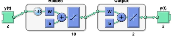
In this section, a deep learning model for predicted gold and silver price is developed. The data used in this section are both gold and silver prices as described in Section 3.1.1. The deep learning model used here is based on the nonlinear autoregressive (NAR) model [33]. This neural network time series tool can be used to predict 𝑦(𝑡) given 𝑑 past values. After the model development, the resulting model takes both the daily gold and silver prices as the input data. The NAR model is configured with 𝑑 = 30 delay periods and 10 hidden neurons as shown in Fig. 9. The NAR network training was done using the Levenberg-Marquardt method [35], [36] by randomly dividing the data into 70%-15%-15% for training, validation, and testing processes, respectively.

Fig. 9. Structure of the NAR model for gold and silver price prediction

The training took 14 iterations with the best mean square error of 6.4282×10-5 _{at 8}th _{iteration. Although}

fit nicely to the normal distribution. This suggests that the model does not overfit and the bias-variance tradeoff is good for the application.

Fig. 10. Error histogram of the silver price prediction. The mean of the error is 3.3×10-3

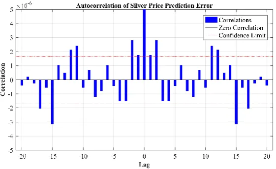
Since the precious metal price prediction is a time-series analysis, it is important to check the error auto-correlation of the silver price prediction which is shown in Fig. 11. There are a few lags that have their corresponding autocorrelation greater than the confidence limit. These lags are the 1st_{, 2}nd_{, 11}th_{, 12}th_{, 15}th_{, and}

17th _{lags. This means that the prediction model could be further improved with additional data and a more}

complicated model.

Fig. 11. Error autocorrelation of silver price prediction.

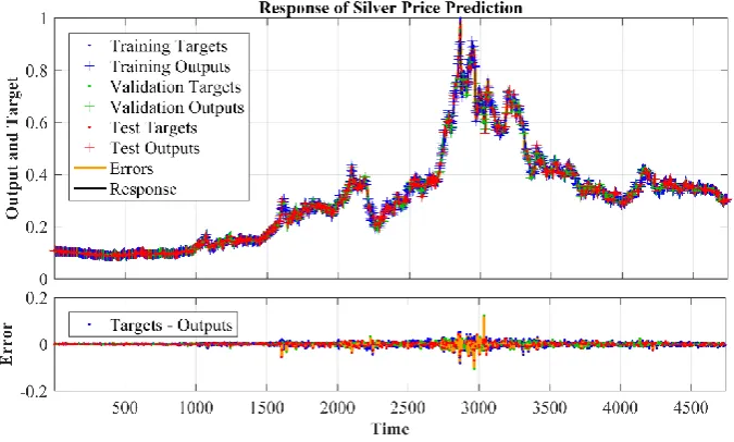
The result of the training is shown in Table 3 and Fig. 12. Using this NAR network, one can easily perform a single- or a multi-step-ahead prediction of gold and silver prices.

Table 3. The training result of the silver price prediction using gold and silver prices as input data.

Target Values RMSE R2

Fig. 12. The response of the output of silver price shows accuracy and error between actual and predicted values.

5.

Machine Learning Model for Diamond Price Forecasting

Similar to the precious metal price, the gemstone price is a key part of the production cost of the jewelry industrial. In this section, we perform predictive analysis of the diamond price using a generalized linear model, a multi-layer feed-forward artificial neural network, a decision tree, a random forest, and a gradient boosted trees model. The results of each model are discussed in the following sections.

5.1. Diamond Price Prediction Using Naïve Forecasting Method

In this section, we create a baseline prediction model for comparison with other models developed later. The naïve forecasting method is a simple technique but works quite well for the forecasting the diamond price. This is because of the diamond price is quite steady and only change a few times over the 10 years of the study.

Considering the histogram of price changes shown in Fig. 3, the jewelry manufacturers can apply the naïve forecasting method described in Section 3.2.1, and they would get approximately accuracy value of (124-8.34)/124 = 0.9327, average RMSE value of 0.03143, and maximum RMSE value of 0.09294. This is the forecasting method commonly used in the industry. Therefore, this accuracy value will be used as the baseline for comparison.

5.2. Diamond Price Prediction Based on Machine Learning Models

In this section, we developed machine learning models to predict the diamond price using RapidMiner Studio [42]. We use the same data described in Section 3.1.2. The price data contains 3,400 series of 124 time-steps with 4 exogenous input elements which are the corresponding 4C parameters. The 12 lags of the delayed input are included as exogenous input as well.

Fig. 13. Root Mean Squared Error of the diamond price of five machine learning models.

5.3. Diamond Price Prediction Based on Deep Learning NARX Model

In this section, we would like to further improve the prediction performance of the diamond price. We still use the same data as the Section 5.1. However, the price data of 12 lags were also considered as the delayed input elements as well.

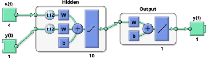
The machine learning model used here is based on nonlinear autoregressive with external (exogenous) input (NARX) [33]. This neural network can be used to predict time series 𝑦(𝑡) given 𝑑 past values and another series 𝑥(𝑡). The neural network is set up as 𝑥(𝑡) are the 4Cs parameter of the diamond, 𝑦(𝑡) are the corresponding diamond's price, 𝑑 = 12 delay periods, and 10 hidden neurons as shown in Fig. 14. The NN training was done using the Levenberg-Marquardt method [35], [36] by randomly dividing the data into 70%-15%-15% for training, validation, and testing processes, respectively.

Fig. 14. Structure of the NARX model for diamond price prediction.

The training stopped at the 11th _{iteration with the value of the mean square error of} 1.37 × 10−4_{, when there}

is an increase in the mean square error of the validation sample after this iteration. The result of the NARX network training is shown in Table 4.

Table 4. The training result of the diamond prices.

Target Values RMSE R2

Training 218,736 0.01177 0.98770 Validation 46,872 0.01229 0.98661 Testing 46,872 0.01812 0.97479

As shown in the error histogram in Fig. 15, the analysis of residue shows a small bias of 3.361×10-3_{. However,}

shown in Fig. 16. This indicates the accuracy and error of the prediction. Using this NARX network, one can easily predict a single or a multi-step-ahead prediction of diamond prices.

Fig. 15. Error histogram of the diamond price prediction. The mean of the error is 3.361×10-3

Fig. 16. The response of the output of diamond price shows accuracy and error between actual and predicted values.

6.

Conclusion

In this work, a material price prediction model of jewelry manufacturers is proposed. The model consists of two separated deep learning models for predicting gold-and-silver price and diamond price. The diamond price model utilizes a novel method to quantize the diamond 4C grade.

The proposed novel quantization method of 4C grades shown in Table 1 is validated by the multiple linear regression and confirmed with visualized plots of the relationship between the 4C parameter with the price. The proposed method considers the cut shape as categorical data and represents it with 1-hot encoding. The color and clarity are considered as discrete data and represented as linearly increasing values as shown in Table 1.

Since the price data is already available in Thailand small jewelry businesses, the proposed model can be easily implemented in the industry.

The proposed diamond price model offers RMSE of 0.0181. Comparing to the naive model that offers RMSE of 0.03143, the proposed diamond price model provides 42.41% improvement. Comparing to the literature, our proposed model can provide a similar order of accuracy while offering less data requirement. This is because the proposed diamond price model only relies on the historical diamond price which is already available in Thai small business jewelry manufacturers.

Comparing the precious metal price model and the diamond price model, there is a big difference in the accuracy of the two models. The precious metal price model offers higher accuracy than the diamond price model because of the amount of data available in this work. In the diamond price analysis Section 5.3, although the data is obtained over the 10 years, there are only 124 time-steps, because it is monthly data. This could be a reason that the R-squared value of the model in Section 5.3 is lower than that of in Section 4 which has over 6,512 time-steps.

The precious metal and diamond price prediction models proposed can be used by small businesses in the jewelry industry to predict their raw material price to manage their production cost. These models can be used in the development of a system dynamics model which can be used to simulate the impact of policy and measure to the industrial.

References

[1] Gem and Jewelry Information Center, “Thailand’s gem and jewelry import-export performance 2018,” The Gem and Jewelry Institute of Thailand, Feb. 2019.

[2] S. Thammaruaksa, W. Saneha, and S. Apirajkamol, “Thai gems and jewelry industries census project,”

University of the Thai Chamber of Commerce Journal, vol. 30, no. 1, 2010.

[3] S. Supacharasai, “Gems and jewelry industries,” in Industrial Competitiveness Enhancement Project under

International Industrial Cooperative Framework. Thai APEC Study Centre, Thammasat University, 2003, ch.

4, p. 87.

[4] T. Somboonwiwat, “Model logistics and supply chain management in gemstone,” 2008.

[5] USAGOLD. (2017). “Gold Prices,” Daily Gold Prices - FOREX Price History, 2017. [Online]. Available: http://www.usagold.com/reference/prices/goldhistory.php

[6] USAGOLD. (2017). “Silver Prices,” Daily Silver Prices - FOREX Price History, 2017. [Online]. Available: http://www.usagold.com/reference/prices/silverhistory.php

[7] S. Sutthichan and M. Suteeraroj, “Factors affected of competitive advantage of gems and jewelry export industries in Thailand,” Nakhon Phanom University Journal, vol. 2, no. 2, pp. 39–45, Aug. 2012.

[8] M. von Saldern, “Forecasting rough diamond prices: a non-linear optimization model of dominant firm behaviour,” Resources Policy, vol. 18, no. 1, pp. 45–58, Mar. 1992.

[9] C. Singfat, “Diamond ring pricing using linear regression,” Journal of Statistics Education, vol. 4, no. 3, 1996.

[10] N. G. Vaillant and F.-C. Wolff, “Understanding diamond pricing using unconditional quantile regressions,” 2013.

[11] B. R. Auer and F. Schuhmacher, “Diamonds—A precious new asset?,” International Review of Financial

Analysis, vol. 28, no. Supplement C, pp. 182–189, 2013.

[12] F.-C. Wolff, “Does price dispersion increase with quality? Evidence from the online diamond market,”

Applied Economics, vol. 47, no. 55, pp. 5996–6009, 2015.

[13] A. Mongkolkaset, “An analysis of foactors affecting the adjustment of gold price,” Master Thesis, The University of the Thai Chamber of Commerce, 2008.

[14] W. Keerativibool, “Forecasting model of monthly gold ornament selling prices,” NU International Journal

of Science, vol. 9, no. 2, pp. 65–81, Jun. 2013.

[15] G. Bandyopadhyay, “Gold price forecasting using ARIMA model,” Journal of Advanced Management Science, vol. 4, no. 2, pp. 117–121, 2016.

[16] S. Shafiee and E. Topal, “An overview of global gold market and gold price forecasting,” Resources Policy, vol. 35, no. 3, pp. 178–189, Sep. 2010.

[18] C. Ciner, “On the long run relationship between gold and silver prices A note,” Global Finance Journal, vol. 12, pp. 299–303, Sep. 2001.

[19] A. Mitra and A. K. Jalan, “Prediction of silver price in volatile market (USD) - based on auto regression integrated moving average,” in Proceeding of the 2014 International Conference on Computing, Communication &

Manufacturing, MCKVIE College India, 2014, pp. 119–130.

[20] W. Jongadsayakul, “Determinants of the gold futures price volatility: The case of Thailand futures exchange,” Applied Economics Journal, vol. 21, no. 1, pp. 59–78, 2014.

[21] W. Jongadsayakul, “Determinants of silver futures price volatility: Evidence from the Thailand futures exchange,” The International Journal of Business and Finance Research, vol. 9, no. 4, pp. 81–87, 2015.

[22] W. Jongadsayakul, “Determinants of the silver futures price volatility: The case of Thailand futures exchange,” in Global Conference on Business & Finance Proceedings, Hilo, United States, 2015, vol. 10, pp. 149–155.

[23] C. Bourne. (2016). “Forecasting with Machine Learning Techniques,” Cardinal Path - Web Analytics and Data

Driven Marketing [Online]. Available:

http://www.cardinalpath.com/forecasting-with-machine-learning-techniques/

[24] S. Mirmirani and H. C. Li, “Gold price, neural networks and genetic algorithm,” Computational Economics, vol. 23, no. 2, pp. 193–200, Mar. 2004.

[25] De Beers, “The Diamond Insight Report 2018,” De Beer Group, UK, 2018.

[26] M. Rapaport. (2017). Rapaport Diamond Price,” Rapaport Diamond Price [Online]. Available: http://store.rapaport.com/price-lists/

[27] International Diamond Exchange. (n.d.). IDEX Diamond Price [Online]. Available: http://www.idexonline.com/diamond_prices_lp

[28] Kitco Metals Inc. (n.d.). Live Gold Price [Online]. Available: https://www.kitco.com/charts/livegoldw.html

[29] Gemological Institute of America Inc. (n.d.). 4Cs of Diamond Quality [Online]. Available: https://4cs.gia.edu/en-us/4cs-diamond-quality/

[30] GIT. (2018). The Gem and Jewelry Institute of Thailand (Public Organization) [Online]. Available: https://www.git.or.th/.

[31] R. J. Hyndman and A. B. Koehler, “Another look at measures of forecast accuracy,” International Journal

of Forecasting, vol. 22, no. 4, pp. 679–688, Oct. 2006.

[32] H. Xie, H. Tang, and Y.-H. Liao, “Time series prediction based on NARX neural networks: An advanced approach,” in 2009 International Conference on Machine Learning and Cybernetics, 2009, vol. 3, pp. 1275–1279.

[33] S. A. Billings, Nonlinear System Identification: NARMAX Methods in the Time, Frequency, and Spatio-Temporal

Domains, 1 ed. Chichester, West Sussex, United Kingdom: Wiley, 2013.

[34] M. Espinoza, J. A. Suykens, and B. De Moor, “Short term chaotic time series prediction using symmetric LS-SVM regression,” in Proc. of the 2005 International Symposium on Nonlinear Theory and Applications

(NOLTA), 2005, pp. 606–609.

[35] K. Levenberg, “A method for the solution of certain non-linear problems in least squares,” Quarterly

Journal of Applied Mathmatics, vol. II, no. 2, pp. 164–168, 1944.

[36] D. Marquardt, “An algorithm for least-squares estimation of nonlinear parameters,” Journal of the Society

for Industrial and Applied Mathematics, vol. 11, no. 2, pp. 431–441, Jun. 1963.

[37] The MathWorks, Inc. (2019). Levenberg-Marquardt backpropagation - MATLAB trainlm. [Online]. Available: https://www.mathworks.com/help/deeplearning/ref/trainlm.html

[38] M. T. Hagan and M. B. Menhaj, “Training feedforward networks with the Marquardt algorithm,” IEEE

Transactions on Neural Networks, vol. 5, no. 6, pp. 989–993, Nov. 1994.

[39] H. I. Erdal, O. Karakurt, and E. Namli, “High performance concrete compressive strength forecasting using ensemble models based on discrete wavelet transform,” Engineering Applications of Artificial

Intelligence, vol. 26, no. 4, pp. 1246–1254, Apr. 2013.

[40] L. Yu, W. Dai, and L. Tang, “A novel decomposition ensemble model with extended extreme learning machine for crude oil price forecasting,” Engineering Applications of Artificial Intelligence, vol. 47, pp. 110– 121, Jan. 2016.

[41] J. Deeying, K. Asawarungsaengkul, and P. Chutima, “Multi-objective optimization on laser solder jet bonding process in head gimbal assembly using the response surface methodology,” Optics & Laser

Technology, vol. 98, pp. 158–168, Jan. 2018.