Development of ANEW 3D euler-lagrange model for the prediction of scour around offshore structures

EULER-LAGRANGE MODEL FOR THE

PREDICTION OF SCOUR AROUND

OFFSHORE STRUCTURES

Thesis submitted in accordance with the requirements of

the University of Liverpool for the degree of Doctor in Philosophy

by

YARU LI

Illustrations v

Notations x

Acknowledgements xiii

Abstract xv

1 Introduction 1

1.1 Initiation of the Study . . . 1

1.2 Aims and Objectives . . . 5

1.2.1 Aims . . . 5

1.2.2 Objectives . . . 6

1.3 Contents . . . 7

2 Literature Review 9 2.1 Introduction . . . 9

2.2 Scour at Offshore Structures . . . 10

2.2.1 Flow Pattern . . . 11

Flow around a Slender Pile . . . 12

Flow around a Pipeline . . . 15

2.2.2 Sediment Transport . . . 17

2.2.3 Scour Process . . . 18

Scour underneath Pipelines . . . 20

2.3 Hydrodynamic Modelling . . . 23

2.3.1 Shallow Water Modelling . . . 24

2.3.2 Computational Fluid Dynamics Modelling . . . 25

2.3.3 Turbulence Modelling . . . 27

Direct Numerical Simulation . . . 28

Large Eddy Simulation . . . 29

Reynolds-Averaged Simulation . . . 31

2.4 Sediment Transport and Scour Modelling . . . 33

2.4.1 Single-phase Model . . . 35

Euler-Euler Method . . . 40

Lagrangian Method . . . 42

Euler-Lagrange Method . . . 43

2.4.4 Treatment of the Solid Phase . . . 45

Drag Force . . . 45

Mixture Viscosity . . . 48

Inter-particle Stress . . . 52

2.5 Conclusions . . . 53

3 Numerical Model 56 3.1 Introduction . . . 56

3.2 Hydrodynamic Module . . . 57

3.2.1 Navier-Stokes Equations . . . 58

3.2.2 Two-Fluid Methodology . . . 59

3.2.3 Existing Terms in Momentum Equation . . . 61

Viscous Stress . . . 61

Body Force . . . 62

Pressure . . . 63

Final Form for Pure Fluid Phase . . . 64

3.2.4 Turbulence Closure . . . 64

3.3 Particle Module . . . 65

3.3.1 Introduction . . . 65

3.3.2 Governing Equation . . . 66

3.3.3 Solid Volume Fraction . . . 69

3.3.4 The Concept of Parcel . . . 70

3.3.5 Drag Force . . . 71

3.3.6 Inter-particle Stress . . . 72

3.3.7 Particle Tracking Method . . . 75

3.4 Coupling of the Fluid Phase and Solid Phase . . . 80

3.4.1 Interphase Momentum Transfer . . . 81

3.4.2 Mixture Viscosity . . . 82

3.4.3 Volume Exclusion Effect . . . 83

3.5 Boundary and Initial Conditions . . . 85

3.5.1 Boundary Conditions . . . 85

3.5.2 Initial Conditions . . . 87

Initialisation of the Parcel Positions . . . 88

3.6 Discretisation and Solution Procedures . . . 89

3.6.1 Discretisation . . . 89

3.6.2 Solution Procedures . . . 96

3.7 Conclusions . . . 97

4 Model Calibration 100

4.2.1 Cases of Various Particle Size . . . 101

4.2.2 Cases of Various Grid Spacing Ratio to Parcel Diameter . . 105

Particle Fall Velocity . . . 105

Interphase Momentum Transfer Term and Volume Exclusion Term . . . 106

4.3 Isolated Block Tests . . . 109

4.4 Extension of the Model Application . . . 118

4.5 Conclusions . . . 120

5 Model Applications 123 5.1 Introduction . . . 123

5.2 Hydrodynamics . . . 124

5.2.1 Vertical Pile under Currents . . . 124

5.2.2 Plunging Waves Test . . . 131

5.3 Sediment Transport . . . 138

5.3.1 Sheet Flow Test . . . 138

5.4 Scour Studies . . . 144

5.4.1 Current-Induced Pipeline Scour . . . 144

Flow Field . . . 145

Turbulence Structures . . . 149

Modified Viscosity . . . 151

Particle Distribution . . . 152

Bed Evolution . . . 153

Influence of Hydrodynamics on Bed Profile . . . 155

Onset of Scour . . . 159

5.4.2 Wave-Induced Pipeline Scour . . . 169

Flow Field and Bed Evolution . . . 170

Particle Distribution . . . 174

5.5 Conclusions . . . 176

6 Discussion, Conclusion and Future Work 180 6.1 Discussion . . . 181

6.1.1 Particle Modelling Approach . . . 181

Advantages . . . 181

Formulation . . . 183

Implementation . . . 184

Validation . . . 187

6.1.2 Euler-Lagrange Multiphase Approach . . . 187

Advantages . . . 187

Implementation . . . 190

6.1.3 Model Application . . . 191

6.2 Conclusions . . . 193

Various Particle Properties . . . 198

Elaborate Implementation of Forces . . . 199

Turbulence-Particle Interaction . . . 200

6.3.2 Model Application . . . 202

6.3.3 Conclusions . . . 203

References 204

List of Figures

2.1 Sketch of the flow pattern around a vertical pile. S refers to the

sepa-ration line. (After Sumer and Fredsøe[80].) . . . 13

2.2 Sketch of the lee wake effect under waves. (After Sumer and Fredsøe[78].) 16 3.1 Sketch of a particle moving from original position a to final position b. (After Macpherson et al.[49].) . . . 77

3.2 Sketch of a computational domain. Red: water; blue: air. . . 86

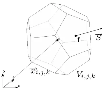
3.3 Control volume. . . 90

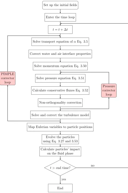
3.4 Flow chart of the solution procedure. . . 98

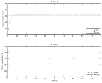
4.1 Computed particle fall velocities in comparison with the theoretical values. . . 104

4.2 Magnitude of the interphase momentum transfer term and volume ex-clusion term. . . 108

4.3 Velocity vector field (left column) and velocity profiles at selected sec-tions (right column) in Tests MDL. Red line: the boundary of the block. . . 113

4.4 Velocity vector field (left column) and velocity profiles at selected sec-tions (right column) in Tests BTM. Red line: the boundary of the block. . . 114

4.5 Velocity vector field in Tests CRN. Red line: the boundary of the block.115 4.6 Velocity difference field. Red line: the boundary of the block. . . 116

4.7 Magnitude of interphase momentum transfer term (left column) and volume exclusion term (right column). . . 117

4.8 Velocity vector field. Red line: the boundary of the wedge. . . 119

sion term. . . 119

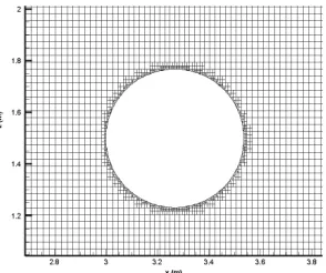
5.1 Refined mesh around the pile. . . 125

5.2 The computational domain. Red: water; blue: air. . . 125

5.3 The developed free surface. Red: water; blue: air. . . 126

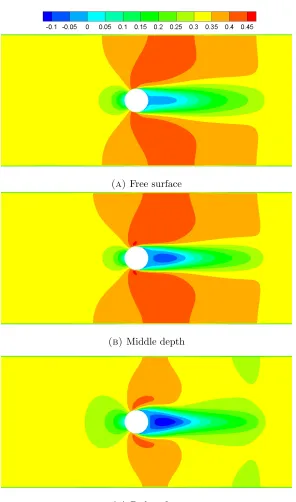
5.4 Streamwise velocity (m/s) distribution at the free surface (A), the middle depth of the flow (B), and near the bed (C). . . 127

5.5 Vertical velocity (m/s) distribution at the free surface (A), in the mid-dle depth of the flow (B), and near the bed (C). . . 129

5.6 Streamwise velocity in the plane of symmetry at different vertical lay-ers. The level heightz is measured from the bed. Solid line: modelling results; asterisks: measurements. . . 131

5.7 Experimental set-up of the plunging wave test by Ting and Kirby[87]. (After Ting and Kirby[87].) . . . 132

5.8 Computational domain. Red: water; blue: air. . . 133

5.9 Snapshot of the computed free surface att = 150s. Red: water; blue: air. . . 133

5.10 Distribution of the wave amplitudes and the mean water surface eleva-tion. Black lines: modelling results; green line: computed mean water level; dots: measurements. . . 134

5.11 Time series of the water surface elevation at selected sections (Part I). Black: modelling results; red: measurements. . . 135

5.12 Time series of the water surface elevation at selected sections (Part II). Black: modelling results; red: measurements. . . 136

5.13 Time-averaged horizontal velocity (u) profile at selected sections. Lines: modelling results; circles: measurements. . . 137

locity w, and turbulent kinetic energy k at selected sections (Part I). Black: modelling results; red: measurements. . . 138

5.15 Phase-averaged surface elevation η, horizontal velocity u, vertical ve-locity w, and turbulent kinetic energy k at selected sections (Part II). Black: modelling results; red: measurements. . . 139

5.16 The velocity profile at selected phases. t/T = 0.0, 0.13, 0.25, 0.4, 0.58,

0.66, and 0.96 as indicated in the figure by each line. Black solid lines:

modelling results; red dashed lines: measurements. . . 140

5.17 Particle distribution and streamwise velocity at selected phases. . . 141

5.18 Comparison of the computed and measured sediment concentration at

various flow phases in the first half of a wave cycle. Lines: modelling

results; circles: measurements. . . 143

5.19 Comparison of the computed and measured sediment concentration at

various flow phases in the second half of a wave cycle. Lines: modelling

results; circles: measurements. . . 144

5.20 Computed flow velocity field at t= 1.5 min. . . 146 5.21 Streamwise velocity and velocity profile at selected sections. Bold solid

line: bed profile. . . 148

5.22 Vorticity magnitude at t = 1.5 min. Bold solid line: bed profile. . . 149 5.23 Sub-grid scale kinetic energy and sub-grid scale eddy viscosity at t =

1.5min. Bold solid line: bed profile. . . 150 5.24 Contour of solid volume fraction (a) and modified viscosity (b) at t=

1.5min. . . 151 5.25 Particle distribution at selected time. a)t= 4 s, b)t = 12s, c) t= 24

s, d) t= 37 s, e) t= 41 s,f) t= 45 s. . . 152 5.26 Computed bed profile at t= 1.5minin comparison with the

measure-ments (black dots). . . 154

5.27 Bed profile and the flow velocity field at selected time. . . 155

ments (black dots). From a) to f) are Test 1 to Test 6 in sequence. . . 157

5.29 Computed flow velocity field at t= 1.5min. From a) to f) are Test 1 to Test 6 in sequence. . . 158

5.30 Detailed flow velocity field at t = 1.5 min in Test 2 (a), Test 4 (b), and Test 6 (c). . . 160

5.31 The initial set-up for simulation of onset of scour. . . 161

5.32 Development of the bed profile and flow velocity field (Part I). . . 162

5.33 Development of the bed profile and flow velocity field (Part II). . . 163

5.34 Development of the bed profile and flow velocity field (Part III). . . 164

5.35 Development of the pressure field. Bold black line: bed profile. . . 165

5.36 Development of the flow field and bed profile. Contour: flow pressure field; vector: flow velocity field; bold red line: bed profile. . . 166

5.37 Development of the bed profile and flow velocity field. . . 172

5.38 Sub-grid scale kinetic energy, eddy viscosity and vorticity at t = 0.5 min. . . 173

5.39 Bed profile comparison against measurements. Red line: modelling result; black dots: measurements. . . 175

5.40 Vorticity and particle distribution (Part I). . . 176

5.41 Vorticity and particle distribution (Part II). . . 177

List of Tables

4.2 Cases of various grid spacing. . . 106

4.3 Theoretical fall velocity and modelling results. . . 106

4.4 Cases of various grid spacing with d50 being 0.36mm. . . 107

4.5 Model set-up in the isolated block tests. . . 110

5.2 Maximum discrepancies observed at the upstream side, scour hole and

downstream side of the pipe in each test. . . 157

6.1 Model applications. . . 192

A particle acceleration

Cd drag coefficient

D cylinder diameter

d50 particle median grain size

Dp parameter related to drag coefficient

g gravitational acceleration

h water depth

k turbulence kinetic energy

ksgs sub-grid scale kinetic energy

KC Keulegan-Carpenter number

n porosity

p subscript for particles

P pressure

Pd dynamic pressure

q sediment transport rate

qb bed load sediment transport

rp particle radius

Re Reynolds number Re viscous stress tensor

ReD pile Reynolds number

Red particle Reynolds number

S equilibrium scour depth S face normal vector

SU momentum source

Simt interphase momentum transfer

t time ∆t time step

T time period of an oscillatory flow

Ts time scale of the scour process

Tve volume exclusion term

Tw wave period U velocity

Uf undisturbed bed shear velocity Uf fluid phase velocity

Up particle velocity

Uw undisturbed orbital velocity

Vp particle volume

x abscissa

x position vector

xp particle position vector

y vertical coordinate

z transverse coordinate

ατ amplification factor

α volume fraction of water

δ bed boundary layer thickness

ε turbulence dissipation

ζ water surface elevation

η Kolmogorov scale

θcr critical Shields parameter

θcs critical solid volume fraction

θf fluid volume fraction

θs solid volume fraction

κ Von Karman constant

λ fraction factor

µ dynamic viscosity

µ0 intrinsic viscosity

µf fluid viscosity

µ0_f modified fluid viscosity

ν kinematic viscosity

νt eddy viscosity

ρ density

ρf fluid phase density

ρp particle density

τ bed shear stress

τp inter-particle stress

τ∞ undisturbed bed shear stress

τ_ijs subgrid-scale stress

φ particle distribution function

ω specific dissipation rate

ωs particle fall velocity

I would like to thank Dr. M. Li, of School of Engineering, The University of

Liv-erpool, for teaching me coastal engineering and scientific writing, and for invoking

my scientific scepticism. I would like to thank Dr. J. M. Harris, of HR

Walling-ford, for teaching me knowledge of scour and scientific writing, and nurturing my

enthusiasm for research. I have been particularly privileged to have both as my

supervisors, who provide me with invaluable advice and guidance, generous

sup-port and patient mentoring throughout my Ph.D. study. I would like to thank Dr.

S. Ilic, of Lancaster Environment Centre, Lancaster University, and Dr. J. Zhou,

of School of Engineering, The University of Liverpool, for agreeing to be my

ex-aminers and for their valuable time, detailed attention and invaluable advice given

to the thesis. I would like to thank Prof. X. Chen, of Ocean University of China,

for teaching me Physical Oceanography, and for his care, patient mentoring, and

invaluable support and guidance. I would like to thank Prof. P. D. Thorne and Dr.

J. Wolf of National Oceanography Centre for teaching me sediment transport and

Physical Oceanography, and for the fruitful discussions and guidance. I would like

to thank Dr. D. M. Kelly of HR Wallingford for his initial input into this work, and

his patient teaching and guidance. I would like to thank Dr. J. R. Finn, of School

of Engineering, The University of Liverpool, for his insightful advice, stimulating

discussions, and inspiring suggestions. I would also like to thank Dr. J. Nicholson,

of School of Engineering, The University of Liverpool, for his encouragement and

inspiration over the small talks on the corridor. In memory of him. I am also very

grateful to the financial support from Engineering and Physical Sciences Research

grandmother for their wholehearted support of my study.

Numerical modelling of scour around offshore structures is still a challenging

re-search topic for engineers and scientists due to the complex flow-structure-seabed

interactions. In comparison to single-phase models and Eulerian models with

Exner equation, a multiphase approach has advantages in interpreting the

flow-particle and flow-particle-flow-particle interactions. In the present study, an Euler-Lagrange

multiphase approach is adopted to develop a new scour model in order to simulate

the air-water-sediment interplay simultaneously while being computationally

effi-cient. The model is able to represent free-surface flow with a mobile bed, which

is often critical for realistic scour modelling. Based on the open source

compu-tational fluid dynamics (CFD) software package OpenFOAM®, the model solves

the Navier-Stokes equations on an Eulerian computational grid. The sediment

particles are traced using the multiphase particle-in-cell (MP-PIC) method in a

Lagrangian approach. The drag force from the fluid, body forces and inter-particle

stresses as well as the interphase momentum transfer are all accounted for in the

model. The model system is calibrated using several simple test cases,

includ-ing a fallinclud-ing particle and steady flow passinclud-ing isolated blocks, to identify optimal

parameters for model operation. The model is then validated against available

ex-perimental data on a steady current around a vertical cylinder and sand suspension

under oscillatory sheet flow, amongst other tests, with satisfactory agreement.

Ap-plication of the model against laboratory experiments includes benchmark scour

The tunnel erosion and lee-wake erosion stages are captured well by the model.

The scour prediction matches with the measurements. In addition, the onset of

scour is reproduced vigorously without any additional numerical assumptions or

approximations. The model’s capability to resolve the scour process and reveal

the mechanisms involved is presented well.

Introduction

1.1

Initiation of the Study

Scour has long been recognised as a severe safety hazard to the structures

con-structed in the fluvial and marine environment. Scour is used to distinguish the

sediment transport process caused by the presence of a structure from the more

general term “erosion”[80]. Scour at bridge piers, for example, has been studied

extensively in the past several decades[8, 23, 36, 38, 52, 59]. Studies on scour in the

marine environment did not gain as much attention until three or four decades ago

when the construction of offshore structures became common, and consequently

the geotechnical guidelines towards scour hazard assessment and scour protection

measures were in urgent needs. In engineering practice, the costs of the scour

pro-tections or remedial measures are often significant, especially in coastal or offshore

projects. As indicated by Whitehouse et al.[92], the scour depth at offshore wind

farm monopile foundations can be as large as 1.38 times the monopile diameter.

More recently, Harris and Whitehouse[21] noted that the scour depth has been

observed up to 2.4 times the monopile diameter, depending on the site conditions. At some sites where scour protections are installed, the edge scour or secondary

scour around the protection can cause even deeper scour than the unprotected

ones[92]. For instance, the scour protection at Scroby Sands off the east coast of

England, has caused unintended expansive secondary scour. Therefore, it is still

a challenging and urgent task to better understand the scour process and develop

better prediction tools to minimise the risks associated with scour at the offshore

structures.

Scour processes in the marine environment are also far more complex under

com-bined waves and currents than those in rivers under currents. The time-varying

nature of the sea, the complexity of the seabed formation, and the presence of

structures on the seabed all contribute to the difficulties of scour study in the

marine environment. For example, the flow dynamics around a structure under

currents, waves, or combined waves and currents are still not fully understood,

including the amplification of the bed shear stress around the structure and in the

ambient flow, the flow separation position with respect to different shape, size,

and orientation of the structure etc. The generation and dissipation of

turbu-lence around the structure and in the lee-wake region are also quite challenging,

which are often critical to the sediment dynamics and the ultimate scour pattern.

Furthermore, the influences of the hydrodynamics and turbulence on the

are yet to be implemented in the commonly used prediction tools. The

mechan-ics of the overall scour process from the initiation to the equilibrium status has

not been properly reflected in existing scour models due to the limitation in the

assumptions and approximations when resolving the sediment dynamics and its

interaction with the flow dynamics.

To tackle these challenges, different approaches have been employed, including

in-situ measurements, physical modelling (laboratory based) and computer

mod-elling. Various numerical modelling approaches can be found in the literature,

including the single phase mixture approach, the Eulerian type approaches, and

the multiphase approaches. Works based on the potential flow theory were

car-ried out at the early stage[41, 43, 50]. However, with the many assumptions and

ad-hoc parametrisations, these models often fail to produce the whole picture of

the sediment transport and scour process. Later on, Eulerian models with Exner

equation were developed to study scour problems with the aid of mesh deformation

or dynamic mesh method to resolve the bed. Due to the limitation in resolving

the flow-sediment interactions, the pick-up of the sediment particles from the bed

and the flow-bed interactions rely on many empirical relations that lead to many

uncertainties in the results. Furthermore, mesh deformation and dynamic mesh

method require special and careful treatment to prevent mesh distortion and

main-tain the mesh quality. Therefore, such models usually struggle to resolve the rapid

changing bed profile and often fail to resolve the shape of the scour hole and the

eroded bed profile correctly, especially where large steepness is observed. Lately,

the multiphase approach is gaining in popularity due to its capability to better

interpret the flow-sediment and sediment-sediment interactions. However, in such

multiphase approach models, usually only the water and sediment are considered,

such models, but also implicates inaccuracy in the scour prediction as the free

sur-face effect is often critical for realistic scour processes especially those under waves

or combined waves and currents. Therefore, incorporating the free surface effect

to achieve a better and more reliable scour prediction is one of the motivations of

the present work.

In multiphase approaches, the flow is often referred to as the fluid phase, and the

sediment is named the solid phase. According to the treatment of each phase,

one of the following methods are usually employed: Euler methods,

Euler-Lagrange methods and Lagrangian methods. In Euler-Euler models, both the

fluid phase and the solid phase are regarded as continuum, thus, the fluid-particle

interactions cannot be resolved directly due to the continuum assumption of the

solid phase, and instead they must be addressed explicitly with parameterisations.

Moreover, Eulerian models are typically based on cell-averaged quantities,

there-fore, they often struggle to model complex deformation and interface

fragmenta-tion. By contrast, in Lagrangian models, such as the Smoothed Particle

Hydrody-namics method (SPH) and the Moving Particle Semi-implicit method (MPS), the

inherent discrete-particle property of sediment is well represented. However, as

the most well-known drawback, Lagrangian models are particularly demanding on

computational resources. Moreover, the incorrect pressure approximation caused

by a spurious pressure fluctuation is a common problem associated with the sharp

fluid interfaces in such models.

Drawing on the advantages of these two types of models, Euler-Lagrange type

mod-els provide an attractive alternative. In such modmod-els, the fluid phase is treated as

continuum on an Eulerian grid, and the solid phase is treated as discrete

interaction between the phases can be resolved straightforwardly. It is also

com-putationally efficient compared to Lagrangian models. Therefore, Euler-Lagrange

models can be a powerful tool to resolve the physics and reveal the mechanics

involved in scour processes. However, the coupling of the Eulerian grid and the

Lagrangian framework, the incorporation of the free surface, the treatment of the

solid phase in flows ranging from very diluted to hyper-concentrated, among

oth-ers, are all challenging tasks, and consequently hinder their application in scour

studies. Considering the outstanding advantages of such models to possibly resolve

the scour mechanics and improve scour prediction, this work is therefore motivated

to develop a novel scour model using the Euler-Lagrange multiphase approach to

study the scour process around offshore structures with the free surface effect.

1.2

Aims and Objectives

1.2.1

Aims

The present work has the following two aims:

1. To develop a novel numerical tool based on the Euler-Lagrange multiphase

approach for reliable scour prediction around offshore structures;

2. To improve the understanding of the scour process and reveal the details of

1.2.2

Objectives

The specific research objectives include:

1. To develop an Euler-Lagrange multiphase approach to resolve the

dynam-ics of the flow field and the bed evolution simultaneously during the scour

process;

2. To develop a particle based approach to represent the sediment dynamics and

the sediment-flow interactions in particulate flow ranging from very dilute

to hyper-concentrated flow, as well as a fully packed bed;

3. To perform scour prediction around offshore structures under different

hydro-dynamic conditions and resolve the detailed processes using the new model;

4. To examine the impact of turbulence characteristics on the scour process;

5. To examine the mechanics of scour development from the initiation to the

later stages.

Based on these aims and objectives, the present work also aims to answer several

fundamental questions regarding the scour process and its numerical modelling:

1. How can the free surface effect and a mobile sandy bed be simulated

simul-taneously with the flow dynamics in a computational fluid dynamics (CFD)

2. How can the flow-sediment interactions be represented effectively in a CFD

model?

3. How does the particle motion initiate in the scour process?

4. How does the flow structure, especially the turbulence characteristics, affect

the scour pattern?

5. How does the particle motion affect the overall scour process?

In particular, the current study will focus on the scour processes around

horizon-tal pipelines on the seabed because of its important implications in engineering

practice and the challenges involved in the numerical modelling.

1.3

Contents

An Euler-Lagrange multiphase approach is adopted in the present study to

de-velop a new particle based scour model in order to simulate air-water-sediment

three-phase interplay simultaneously and to reveal the scour mechanism. The

model is able to represent free-surface flow over a mobile bed, to eliminate the

inaccuracy caused by the rigid lid assumption. Based on the open source CFD

software package OpenFOAM®, the model solves the Navier-Stokes equations on

an Eulerian computational gird. The sediment particles are traced using the

mul-tiphase particle-in-cell (MP-PIC) method in a Lagrangian framework. The flow

and sediment particles are fully coupled, and particle-particle interaction is also

In this work, a detailed literature review is presented in Chapter 2. Chapter 3

describes the theories involved in the numerical model. The model calibration is

presented in Chapter 4. Then the results of the model application are presented

Literature Review

2.1

Introduction

In this chapter, the physical processes involved in the scour process, including

the flow regime, sediment transport and scouring, will be reviewed first. Then

the review on the numerical modelling approaches concerning the hydrodynamics,

including the turbulence modelling, and sediment transport and scour, including

the treatment of the solid phase in the multiphase approaches, will be presented

in sequence.

2.2

Scour at Offshore Structures

The presence of structures in the marine environment will change the flow patterns,

turbulence properties, and local sediment transport in its immediate

neighbour-hood, resulting in local scour and further influence on the global scour pattern.

Several phenomena are usually identified, such as flow contraction, a horseshoe

vor-tex in the upstream side, lee-wake vortices and/or vorvor-tex shedding in the

down-stream side, turbulence enhancement, wave reflection, diffraction and breaking

etc.[80]. These changes in the flow field can amplify the local bed shear stress

and enhance sediment transport capacity, which leads to a divergence of sediment

transport rate and ultimately the occurrence of scour.

Conventionally, scour is classified according to different criteria. These terms

below are usually used in scour studies.

ˆ Local scour and global scour. For example, in the case of a multi-leg jacket

structure, the scour pits around each single piles are referred to as local scour;

the saucer-shaped depression beneath and around the whole installation is

called the global scour.

ˆ Clear-water scour and live-bed scour. If the Shields parameter θ (Eq. 2.1) is lower than its critical value θcr, which means that there is no sediment transport in the far area, it is called the clear-water scour; otherwise, when

θ = U

2

f

g(s−1)d, (2.1)

whereg is the gravitational acceleration,sis the specific gravity of sediment grains, d is the grain size, and Uf is the undisturbed bed shear velocity expressed by Uf =

q_τ

∞

ρ , and τ∞ is the bed shear stress for the undisturbed flow. The critical value of the Shields number is a function of the grain

Reynolds number.

2.2.1

Flow Pattern

Despite of the undisturbed flow regime, the flow pattern in the scour process

largely depends on the shape and size of the structure presented in the flow.

Vertical piles and horizontal pipelines are very common structures in the marine

environment. In terms of piles, Sumer and Fredsøe[80] categorise it into two flow

regimes: the slender-pile regime where the pile diameterDis small compared with the wave length L, and otherwise the large-pile regime. The distinguished feature of the former regime is the flow separation with the presence of separation vortices,

which applies to the flow around offshore structures like monopiles in the offshore

Flow around a Slender Pile

A schematic sketch of the slender pile regime is shown in Figure 2.1. When flow is

approaching the pile, the flow structure in the bed boundary layer will be affected

immediately. Induced by the adverse pressure gradient upstream of the pile, the

bed boundary layer separates and a separation line is formed. The separated

boundary layer further generates a horseshoe vortex at the upstream side. In the

case of a steady current, Baker[4] indicates that the ratio of the bed boundary layer

thickness δ to the pile diameter D, i.e., _Dδ, the pile Reynolds number ReD = U D_ν , the bed boundary layer Reynolds numberReδ = U δ_ν , and the pile geometry (shape and size, etc.) are the main parameters to evaluate a horseshoe vortex. The larger

δ

D, ReD, and Reδ are, respectively, the larger the vortex length xs will be. The cross-sectional shape of pile also influences horseshoe vortex by its impact on the

adverse pressure gradient. Generally speaking, it is more difficult for a streamlined

cross-sectional shape to induce large horseshoe vortex. Sumer et al.[77] studied

the impact of square-shaped (90°orientation), circular-shaped and square-shaped

(45° orientation) cross-sectional piles and found out that the square pile with 90°

orientation was the easiest one to generate longerxs. With respect to pile height, the larger _HL (Lis the cross-flow dimension of the pile andH is the pile height) is, the smaller vortices are generated.

Regarding the horseshoe vortex generated under waves, the Keulegan-Carpenter

Figure 2.1: Sketch of the flow pattern around a vertical pile. S refers to the

separation line. (After Sumer and Fredsøe[80].)

KC = UmTw

D (2.2)

where Um is the maximum value of the undisturbed orbital velocity at the bed and Tw is the wave period. It is difficult for the horseshoe vortex to form if KC number is very small; and ifKC number is large, the horseshoe vortex is supposed to behave almost in the same way as in the circumstances of steady flows. Sumer

et al.[77] studied the horseshoe vortex under waves with differentKCnumbers and revealed the impact of KC number on horseshoe vortex by exploring the adverse pressure gradient using the potential flow theory. Their experimental results show

that a KC number smaller than 6 will suppress the boundary layer separation in front of a circular pile. In the case of a square pile with 90°orientation, horseshoe

In the case of waves with a superimposed current, a horseshoe vortex comes into

being more easily. Only a small KC number is required, and the separation distance increases remarkably compared to a case with waves only.

Bed shear stress beneath the horseshoe vortex is an important parameter

asso-ciated with the scour process. The value of the bed shear stress compared to

its undisturbed value is mainly determined by the strength of the horseshoe

vor-tex, and it generally peaks at the side edge of the pile. The study by Baker[4]

on laminar flows indicates that with the presence of a horseshoe vortex, the bed

shear stress can be amplified by a factor of 5−11 compared to the undisturbed

conditions. The study by Hjorth[27] shows that the amplification factor under

the combined action of the horseshoe vortex and the flow contraction effect can

be as large as 11 at the midway between the front and side edges of the slender

pile, which in consequence will lead to dramatically enhanced sediment transport

capacity and scour development around the pile. Under waves, the amplification

factor of the bed shear stress is found to be a function ofKC number, and the bed shear stress increases as KC number increases. Sumer et al.[77] indicate that the transition of a laminar horseshoe vortex into the turbulence regime is dependent

onKC number as well as _Dδ and ReD. In the experiments by Sumer et al.[77], the transition occurred when KC number was between 10 and 20.

The lee-wake vortices are formed at the downstream side of the pile. In steady

currents, the lee-wake flow is mainly determined by ReD and the pile geometry, while under waves, the KC number is a more dominant parameter. Sumer and Fredsøe[84] and Sumer et al.[77] point out that compared to steady-current case,

the lee-wake vortex flow is a more essential component for the scour development

Flow around a Pipeline

Apart from vertical piles, the scour around horizontal pipelines on the seabed has

also been studied extensively in the past. The flow around a pipeline is relatively

simpler than that around a vertical pile. The seepage flow underneath the pipe

and the lee-wake effect are the most predominant features. Driven by the pressure

difference between the upstream and downstream side of the pipe, a seepage flow

will take place underneath the pipeline. It acts as the agitating force on the sand,

and when it exceeds the submerged weight of sand, piping will occur. Sumer et

al.[85] measured the pressure gradient around pipelines in a steady current and

it is found to be increasing with an increasing flow velocity. Sumer et al.[85] also

derived the critical condition of the pressure gradient for piping to occur. Their

study indicates that the excessive seepage flow and the resulting piping are the

major mechanisms to induce onset of scour, which is the initial stage of scour

development around a pipe.

In the case of waves, Sumer et al.[85] measured the surface elevation and the

pressure gradient underneath the pipe. The measurements show that there is a

20−25° phase lag in the pressure gradient compared to the surface elevation. In

addition, the pressure gradient large enough for piping to occur is only available

for a short time during each crest half period. Only after several such exposures,

piping takes place.

In addition to the seepage flow, the lee-wake effect also plays an important role.

Chapter 2. Literature Review 16

region, the vortex shedding becomes less pronounced, which might lead to a smaller lee-wake erosion and hence less scour depth.

As far as the influence of 9 is concerned, this must be examined in two different categories: the clear-water case, where the sediment far from the pipe is not moving, and the live-bed case, where sediment is transported far from the pipe. In the clear water case, the variation in scour depth with 9

is more pronounced: as S/D increases from 0 at very small 9-values up to

values of 0.4-1.0 when the 6-value approaches the live-bed case. However,

when the live-bed case is obtained, very small variation in S/D is observed,

as seen from Fig. 2. Kjeldsen et al. (1973) indicate that S/D increases with

8 by a power of 0.2, while others simply disregard this very weak variation. This variation is weak, because any change in 9 results in corresponding changes in sediment transport. These changes occur upstream of the scour hole and inside the scour hole in equivalent amounts, eventually causing practically no change in the equilibrium scour depth.

SCOUR IN TIDAL FLOW AND WAVES

This section considers the case where flow attacks the pipe from both sides due to near-bed flow induced by wind waves or by slowly varying unsteady current conditions like a tidal current. The main difference between this case and the steady case is that the downstream-formed wake system now occurs on both sides of the pipeline. Here the strong lee-wake erosion, which gives

(a) _Current

Lee-Wake

(b) Waves

FIG. 3. Lee-Wake Effect: (a) Currents; (/>) Waves

310

J. Waterway, Port, Coastal, Ocean Eng. 1990.116:307-323.

Downloaded from ascelibrary.org by University of Liverpool on 08/26/15. Copyright ASCE. For personal use only; all rights reserved.

Figure 2.2: Sketch of the lee wake effect under waves. (After Sumer and

Fredsøe[78].)

found that the lee-wake effect is the key mechanism in this process. Figure 2.2 was

depicted by Sumer and Fredsøe[78] to show the difference of the lee-wake effect

under steady currents and waves respectively. They summarise that the upstream

side of the pipe under a steady current is dominated by potential flow whereas

flow separation and a vortex street, which is formed by the lee-wake vortices, are

observed at the downstream side. Under waves, the lee-wake vortices are observed

at both side of the pipe due to flow reversal during wave cycles as shown in

Figure 2.2[78]. They point out that the extension of the lee-wake vortex street Lv under waves is governed by the KC number, and a linear relation is developed by them according to the flow visualisation study by Jensen and Jensen[31] that

Lv

2.2.2

Sediment Transport

According to the transport mechanism of bed materials, two mechanisms are

iden-tified, namely the suspended load and the bed load. The bed load has continuous

contact with the bed, of which the particles roll, slide or saltate along the bed.

Its transport is almost totally determined by the effective bed shear stress. When

the bed shear velocity just becomes larger than the critical value for the initiation

of motion, the particles will roll and slide, and saltate if the bed shear velocity

continues increasing along the bed, in the regime of bed load transport. Once the

value of the bed shear velocity exceeds the fall velocity of the particles, they will

become suspended in the flow and transfer into the suspended load mode. The

total sum of the bed load and the suspended load is named the total sediment

load.

The Shields number (Eq. 2.1) is an indicator of the initiation of motion for

sed-iment particles. The sediment particles will move once the Shields number θ

exceeds its critical valueθcr, which is given by,

θcr =

U_{f c}2

g(s−1)d, (2.3)

With the presence of structures, the entrainment of bed materials, the transport

capacity of both the suspended load and the bed load are enhanced due to the

enhanced bed shear stress and stronger turbulence level around the structures.

The amplification factorατ is used to measure the increase in the bed shear stress, which is given by

ατ =

τ τ∞

, (2.4)

where τ is the enhanced bed shear stress and τ∞ is that for the undisturbed

flow. Certain amount of knowledge about the enhanced bed shear stress has been

accumulated, some of which are already reviewed in Section 2.2.1. Sumer and

Fredsøe[80] adopted a formulaqb ∼τ3/2 in the discussion of the bed load sediment transport due to bed shear stress. Although this formula is not strictly derived,

it demonstrates the importance of the bed shear stress to bed load transport.

However, there is still little knowledge on the enhanced turbulence level in the

vicinity of the structure as well as its contribution to the sediment transport and

scour processes.

2.2.3

Scour Process

bed. The scour process continues until ατ = O(1) around the structures when the equilibrium stage is reached. The scour depth at that moment is called the

equilibrium scour depth. The time required for the scour development is called

the time scale of the scour process. Sumer and Fredsøe[80] adopt a formula to

represent the time variation of the scour depth,

St=S(1−exp(−

t Ts

)), (2.5)

whereSis the equilibrium scour depth andTsis the time scale of the scour process.

In the case of steady currents, Sumer and Fredsøe[80] point out that the scour

depth is influenced by such factors as the Shields number, the sediment gradation,

d D,

δ

D, the cross-sectional shape and the alignment factor. Regarding the scour

under waves, the study by Sumer et al.[81] indicates that the KC number is the main parameter governing the scour development on a live bed. In terms of

the scour development in combined wave and currents, Sumer and Fredsøe[79]

obtained an empirical expression concerning the scour depth in live bed regime

from experiments with KC <30, which is given by

S D =

Sc

where Sc is the scour depth in steady current alone, and the coefficients A and B are given by

A= 0.03 + 3 4U

2.6

cw, (2.7)

B = 6−4.7Ucw_{, (2.8)}

where Ucw= _UcU₊c_Um, and Uc is the current velocity andUm is the maximum value of the undisturbed orbital velocity at the bed.

Scour underneath Pipelines

In the scour processes underneath pipelines, three stages are usually identified:

onset of scour, tunnel erosion, and the lee-wake erosion stage. Other

three-dimensional processes like the self-burial and backfilling process along the free span

areas and at span shoulders have also been summarised by Sumer and Fredsøe[80].

Previous studies show that the onset of scour is basically related to the seepage

flow in the bed underneath the pipeline, which is caused by the pressure difference

between the upstream and downstream sides of the pipeline[50, 80]. Sumer and

pressure gradient underneath the pipeline, and found that onset of scour is largely

caused by the pressure-gradient driven seepage flow and the resulting piping. A

criterion for onset of scour is given in the study by Sumer and Fredsøe[79] as

follows,

U2

gD(1−n)(s−1)

cr

≥f(e

D), (2.9)

where U is the undisturbed flow velocity at the top of the pipeline, D is the pipeline diameter, n is the porosity, s is the specific gravity of sand, e is the burial depth, and the function f on the r.h.s. is determined by experiments. This non-dimensional form is derived from the following equation, which means that the

critical condition occurs when the pressure gradient _∂x∂ (_γp) outweighs the floatation

gradient (s−1)(1−n)[79]:

∂ ∂x(

p

γ)≥(s−1)(1−n), (2.10)

where γ is the specific weight of water.

When a breach is formed underneath the pipe and it gradually develops into a very

narrow tunnel, the tunnel erosion stage starts. At this stage, the gap between the

However, a considerable amount of water can be diverted through this pathway

towards the downstream side. As the velocity is large in the gap, and the shear

stress can be increased dramatically, and in consequence the sediment transport

there is enhanced considerably. Therefore, at this stage, the scour underneath

the pipe develops substantially and the gap between the bed and the pipeline

is increased fairly quickly. As the gap becomes larger, the flow velocity in the

gap will slow down and this intense scour process will slow down as well. When

the gap reaches a certain depth, the tunnel erosion stage will be followed by

lee-wake erosion, where the bed downstream of the pipe being eroded by the lee-lee-wake

vortices becomes the most prominent feature. Sumer and Fredsøe[80] and Sumer

et al.[83] point out that although the organised wake flow, which is formed by

the agglomeration of separation vortices shed and convected steadily downstream,

takes control of the scour process at this stage, vortex shedding happens from a

very early stage. This process continues until the equilibrium stage is reached

where the bed shear stress underneath the pipeline stays constant and equals to

the undisturbed value, i.e.,τ =τ∞; or in other words by Sumer and Fredsøe[78], it

happens when the sediment transport just below the pipe equals to that far from

the pipe.

Sumer and Fredsøe[78] point out that the scour profile under a steady current

is featured by a steep upstream slope and a gentle downstream slope due to the

different local flow pattern. The upstream side is dominated by a potential flow

whereas the downstream side is featured by a vortex street over a long stretch.

Sumer and Fredsøe[78] also clarify that the downstream side is eroded more

heav-ily due to the higher turbulence level and higher instantaneous velocity. Sumer

et al.[82] found out via experiments that the instantaneous velocity of the

down-stream vortices can be larger than the undisturbed velocity by a factor of 2 or

of scour happens almost at the same time as the passage of a wave crest. The

breakthrough under waves is a more progressive process due to the oscillatory

na-ture of the flow. As reviewed in Section 2.2.1, the extent of the lee-wake vortex

street is dependent on the KC number, Sumer and Fredsøe[78] indicate that the larger the KC number is, the longer the streamwise extent of the bed is affected by the lee-wake vortices during one half-period of the wave cycle. Again due to the

oscillatory nature of waves, the gentle slope being eroded by the lee-wake vortices

happens at both sides of the pipe.

2.3

Hydrodynamic Modelling

A reliable prediction of the hydrodynamics is a prerequisite of a well-functioning

scour model. Two dimensional scour models can give quick assessment of the scour

patterns and predict the maximum scour depth relatively accurately[47]. They are

usually based on the water-depth-averaged shallow water equations (SWEs) and

sediment transport equations. For a better interpretation of the three dimensional

processes, CFD models solve the three-dimensional Navier-Stokes equations

di-rectly, describing the three-dimensional nature of the scouring process without

any hypotheses. Compared to the shallow water modelling, obviously, CFD

mod-els are more capable of capturing the complex hydrodynamics around structures

2.3.1

Shallow Water Modelling

Although it cannot resolve the detailed development of the flow pattern, turbulence

structures or scour characteristics, two dimensional models have their advantages

in giving quick assessment of the main scour parameters with relatively sufficient

accuracy and they are less demanding on computational resources.

The shallow water equations have been employed in most two dimensional models

to simulate the hydrodynamics. With the hydrostatic assumption and the

as-sumption of constant velocity over the water depth, no pressure term is included

in the shallow water equations. Accuracy in second and higher order has been

achieved with the finite volume methods[2, 96]. However, as its name suggests,

shallow water modelling is only applicable to very limited range of scenarios where

the horizontal length scale is much greater than the vertical length scale.

Liu et al.’s model[47] is a typical one using the shallow water modelling approach

by coupling the shallow water equations with the sediment transport equation on

an unstructured mesh. The Godunov scheme was employed to capture the steep

water surface elevation gradient, which was split using the method proposed by

Rogers et al.[68] and Rogers et al.[69] to obtain the hyperbolic formulation. The

inviscid fluxes were solved by Roe’s approach[66, 67], an approximate solver of

Rie-mann problem. Hydrodynamic test of dam break flow in channels with a 90°bend

was performed with fairly good prediction of the free surface compared to

experi-mental data. When it comes to scour modelling, the hydrodynamic performance

resolved well and a recirculation zone was captured in the results. However, due to

the two-dimensional nature of the shallow water equations, three-dimensional

fea-tures such as the horseshoe vortex cannot be resolved, which is a major drawback

to the scour prediction. Moreover, it was problematic of Roe’s approach to cope

with dry-wet interfaces. In addition, scour process usually involves complex

tur-bulence structures, but no turtur-bulence model was employed in their model. There

are many other shallow water approach based models, but the overall structure

and method are similar to those in Liu et al.[47]. No further details are reviewed

herein.

2.3.2

Computational Fluid Dynamics Modelling

Without the assumptions made in shallow water equations, the three-dimensional

Navier-Stokes equations can be solved directly by CFD methods. In scour

mod-elling, the free surface variations often need to be taken into account, such as the

surface gradient induced secondary flow around a bend in open channels and free

surface waves induced scour. However, in cases where the surface variation does

not cause significant effects, the rigid lid method is often applied for simplicity.

Currently, to resolve the free surface effect, the marker and cell method (MAC),

the volume of fluid method (VOF)[26] and the level set method[72] are available

in the literature. In the simulation of multiphase flow, the VOF method has been

widely used. In particular, it has been employed in several scour studies[46, 65].

in steady currents using a three-dimensional finite element model. The

Reynolds-Averaged Navier-Stokes equations (RANS) were solved by the Arbitrary Lagrangian

Eulerian (ALE) scheme and the free surface effects are ignored by using a rigid

lid approximation. They extended the Petrov-Galerkin finite element scheme to

three-dimensional. The weighting function was modified to realise upwind,

mak-ing the upstream value a computational node larger than the correspondmak-ing

down-stream value. It is noteworthy that they calculated a separate case of flow in a

long straight channel (200D long), and used the velocity, sediment concentration

and turbulent quantities at the outlet boundary as the input for the scour model.

Standard wall function was employed in the bed boundary conditions for

com-putational efficiency. The horseshoe vortex and vortex shedding were captured

well by the model, no comparison with flow measurements was presented though.

However, the predicted scour depth along the cylinder perimeter was 10% to 20%

smaller than the measurements. Moreover, the bed shear stress enhancement was

underestimated in the validation test. This could be probably caused by the rigid

lid approximation, as well as the inappropriate treatment in the wall function,

among other simplifications.

Zanganeh et al.[98] investigated current-induced live-bed scour beneath marine

pipelines at tunnel erosion and early stages of lee-wake erosion. The flow was

sim-ulated with the Smoothed Particle Hydrodynamics (SPH) method in a Lagrangian

two-phase model. They adopted the Sub-Particle Scale (SPS) model as the

turbu-lence closure scheme for the flow. The hydrodynamic performance reached good

agreement with experimental data in the upstream and downstream part of the

pipe while the velocity around the pipe was under-estimated. It could be due to

Tofany et al.[88] studied numerically the influence of the breakwater steepness on

the hydrodynamics under standing waves and the scour pattern in front of

im-permeable breakwaters. Their model solves the RANS equations closured by the

k−ε turbulence model for the hydrodynamics. The VOF method was employed to capture the free surface. The predicted near bottom velocity was in good

agree-ment with the experiagree-mental data. However, an additional term of bottom shear

stress had to be included in the momentum equation according to Karambas[32]

such as to achieve a physically sensible scour pattern.

2.3.3

Turbulence Modelling

In scour process, as highlighted previously, the flow tends to be in high

turbu-lence flow region. Vortex shedding and turbuturbu-lence generation/dissipation are very

important processes that often are deterministic to the final scour pattern. To

accurately model the turbulence level is therefore a key factor in the

hydrody-namic simulation. A variety of turbulence models are available to simulate the

turbulence generation and dissipation processes for the flow field, including direct

numerical simulation (DNS), large eddy simulation (LES) and Reynolds-averaged

Direct Numerical Simulation

Direct numerical simulation solves the Navier-Stokes equations directly after

nu-merical discretisation without any averaging or approximation. It gives detailed

information about the velocity and pressure among other variables of interest at

numerous grid points. The results are so detailed that they can even be treated

as equivalent to experimental data and can be adopted for statistical use.

More-over, DNS can control external variables like the wall roughness easily, while it

may be very difficult or even impossible to accurately control some variables in

the laboratory. Hence, it is a great tool to understand the physical mechanisms of

turbulence production and dissipation.

However, this huge amount of information may be unnecessarily sufficient to

coastal engineers, especially considering the large amount of effort needed in

post-processing, let alone the very high expense of computational resources for the

simulation. In order to capture all the significant structures in turbulence as

well as all the kinetic energy dissipation, the computational domain is required

to be no smaller than the physical prototype or the largest turbulent eddy, while

the grid size must be no larger than a viscosity determined scale — Kolmogorov

scale. Even in case of homogeneous isotropic turbulence, the cost of simulation

scales as large as Re3_l[15], where Rel is the Reynolds number with respect to the velocity fluctuations and the integral scale l. Therefore, it is less applicable to high-Reynolds-number simulations. On top of that, the time-advance methods,

the generation of the initial and boundary conditions, among other numerical

is-sues are also challenging. Hence, its application in scour studies has hardly been

Large Eddy Simulation

Turbulent flows contain a wide range of eddies, and the large scale ones are more

effective in the transport of conserved properties. It could be a sufficient solution

to most turbulence simulations that the large scale eddies are resolved directly,

and the less effective small scale eddies are simply parameterised. LES is based on

this hypothesis. LES is three-dimensional and time dependent, producing detailed

turbulence structures, and it is much less expensive than DNS. Hence, it is more

suitable in situations where the Reynolds number is too high and the geometry is

too complex for DNS.

The sub-grid scale (SGS) stress τs

ij is an important concept introduced in LES

models for approximation, which is given by τ_ijs =−(uiuj−uiuj). It is the large scale momentum flux caused by the unresolved scales. It contains information

about local averages of the small scale field. There are several SGS modelling

concepts, based on which several LES models are developed such as Smagorinsky

models, dynamic models and deconvolution models.

LES models require less computational resources than DNS, and it can reproduce

a desirable amount of turbulence information. Although its application in coastal

engineering field is still at its early stage due to the limited computational resources

and numerical techniques, with its outstanding advantage and the rapid progress

in the computational technologies, the application of LES in scour studies has

started emerging in recent years. In particular, Li and Cheng[42] indicate that

their own research and that of others[7, 43].

Nguyen and Wells[54] studied the bedform development under turbulent flow

us-ing a coupled LES and Immersed Boundary Method (IBM) to resolve the

three-dimensional flow field. The SGS stress was computed using the shear-improved

Smagorinsky eddy viscosity model by Leveque et al.[40]. The computed shear

stress distribution over a sinusoidal bed surface was compared to DNS results

with fairly good agreement. The mean flow fields including the streamwise

veloc-ity, the vertical velocveloc-ity, the turbulence kinetic energy and the Reynolds stress all

agree well with the DNS results.

Kim et al.[35] studied the local scour at two adjacent cylinders under clear-water

scour conditions using a combined hydrodynamic-sediment-trasnport-morphodynamic

model. The three-dimensional hydrodynamics was resolved using LES with a

Smagorinsky sub-grid model combined with IBM. The time-averaged velocities

and turbulence intensities in the flow through two vertical cylinders agreed well

with the experimental data, even in front of and behind the cylinders. The

ve-locity spike near the bed behind the cylinder due to the high momentum flux

resulted from the transfer of vortices into the wake region was captured by their

LES model. The relatively high turbulence intensity behind the cylinder due to

vortex shedding was also resolved. In their study, Kim et al.[35] also indicate that

the presence of the cylinders are the principal source of turbulence rather than the

bed friction. The good agreement demonstrates the strength of LES in dealing

Reynolds-Averaged Simulation

Even less demanding on the computational resources, in RAS models, variables in

a statistically steady flow can be expressed as the sum of a time-averaged quantity

and a fluctuation. The eddy viscosityνt is introduced to represent the unresolved scales. Different models have been developed to compute νt, including the k−ε model, k−ω model, and k−ω SST model.

k−ε Model

Thek−εmodel has been adopted for turbulence modelling in a number of sediment transport and scour models[19, 46, 88, 93, 99, 100, 103]. A number of damping

functions have been developed for various applications with thek−εmodels so far, and results agree well with DNS data. The k−ε models are proven to be suitable for flows with small pressure gradients, such as free-shear layer flows, wall-bounded

and internal flows where the mean pressure gradients are small[6].

Liu and Garcia[46] studied wall jet scour using the k − ε model as the turbu-lence closure. The strong jet-induced recirculation behind the sluice gate, small

isolated circulation areas, and the circulation zone inside the scour hole were all

captured well by their model. The momentum diffusion along the abscissa

direc-tion was resolved as well. The horizontal velocity along the abscissa agreed well

with the experimental data, whereas the velocity far downstream of the jet inlet

However, in flows with large adverse pressure gradients, the performance of k−ε

models is declining. It was also commented by Liu and Garcia[46] that two

equa-tions models such as k −ε models can become unstable when simulating wave driven orbital motions, especially when the wave is strong or where wave breaking

takes place. Mayer and Madsen[51] performed analytical stability analysis of the

k −ε model under waves, and found out that the turbulent eddy viscosity be-came unbounded. Hence, they proposed a modified two-equation model for waves,

whereas most models rely on the tuning of the empirical parameters[46] when

using the k−ε model.

k−ω Model

Thek−ωmodel is also a popular choice, especially in the sublayer of the boundary layer[53]. Different from the k−εmodel, k−ω model does not implicate damping functions, and simple Dirichlet boundary conditions can be specified[53]. With

its accuracy in predicting the mean flow profiles as well as its numerical stability,

the k−ω model has also been widely adopted[16, 34]. Moreover, k −ω model produces better results in the logarithmic part of the boundary layer than k−ε

model in adverse pressure gradient flows as reported in the literature.

k−ω SST Model

layers andk−εmodel in the outer regions to avoid the strong free stream sensitivity of the originalk−ωmodel. The latter modifies the definition of the eddy-viscosity in the BSL model to represent the effect of the transport of the principal turbulent

shear stress and remarkably improves the modelling results in adverse pressure

gradient flows as found out by Menter[53] and Zhao et al.[101].

Due to its good performance in flows with strong adverse pressure gradient, the

k−ω SST Model has been a popular choice for scour models[10, 101, 102, 104]. Zhao et al.[101] studied the local scour around a submerged vertical cylinder in

steady currents with the k − ω SST turbulence closure model. The modelled pressure distribution upstream of the pile along the stagnation line and along the

abscissa respectively agreed well with the experimental data. The time-averaged

bed shear stress distribution along the symmetry line upstream of the pile was also

reproduced well, the bed shear stress very close to the pile was underestimated

though.

2.4

Sediment Transport and Scour Modelling

Like the modelling of hydrodynamics and turbulence, the prediction of sediment

transport and scour processes are also dealt with by various approaches

depend-ing on the focus of the individual work as well as the available numerical methods

at the time, which now can be largely divided into single phase and multiphase

stage[41, 43, 50]. However, with the massive assumptions and ad-hoc

parame-terisations, these models often fail to produce the whole picture of the sediment

transport and scour process; only certain aspects of the problem, such as scour

depth at the upstream side, can be predicted reasonably. Later on, the Eulerian

approach with Exner equation type models emerged. In such models, the

govern-ing equations of flow and sediment transport equations are solved on an Eulerian

grid, and the sediment continuity equation, i.e., Exner equation, is used to resolve

the bed elevation. Such models are capable of resolving the scour process with

more detailed calculation compared to the single-phase models. However,

empiri-cal or semi-empiriempiri-cal formulas are still indispensable in such models, and the mesh

deformation or dynamic mesh approach used to resolve the bed elevation is a major

difficulty. Therefore, such models often struggle to resolve the rapidly changing

bed profile, the maximum scour depth is usually underestimated, and the bed

profile is much milder due to the limitation of mesh deformation. Deterministic

models and stochastic models have also been used for scour prediction. However,

the former usually involves many uncertainties because of the empirical nature;

and the latter usually requires a large amount of data prior to model

develop-ment, and a number of assumptions have to be made to determine particle motion

as the forces are usually not calculated directly. In recent years, the multiphase

approach is gaining in popularity due to its capability to better interpret the

flow-sediment and flow-sediment-flow-sediment interactions. In multiphase approach, the mesh

deformation is no longer necessary to resolve the bed. According to the

treat-ment of each phase (solid phase and fluid phase), one of the following methods are

usually employed: Euler-Euler methods, Euler-Lagrange methods and Lagrangian

methods.

In multiphase approaches, the coupling between the the solid phase and fluid

fraction of the solid phase θs and the mass loading φm, which is the mass ratio of the solid phase to the fluid phase, are the two determinant parameters with

respect to the interaction level between the two phases[5]. When θs and φm are small, only the influence of the fluid phase on the solid phase is predominant,

thus one-way coupling is sufficient. When the mass is comparable between the

two phases, the influence of the solid phase back on the fluid cannot be neglected,

two-way coupling is therefore needed. If the volume fraction of the solid phase

increases to a critical value, the particle-particle interactions such as inter-particle

stress and collision become more notable and thus four-way coupling is required.

2.4.1

Single-phase Model

Single-phase models are usually based on the potential flow theory and

viscosi-ty/turbulence closure models. They are able to predict the maximum scour depth

and the upstream session of the scour hole, yet their prediction ability of the scour

profile are largely restricted. Moreover, although some fluid-particle interaction

effects can be considered by the addition of an extra production term in the

tur-bulence model equations, single-phase models are usually not capable to account

for the particle-particle interaction.

Li and Cheng[41] developed a numerical model to simulate the equilibrium scour

hole in clear-water scour based on the potential-flow theory. The Laplace equation

of the flow velocity potential was solved for the fluid phase and the free surface

as the bottom boundary condition to the flow, and it was determined by the

force balance acting on a particle. Therefore, no particle-particle interaction was

interpolated in the model. Moreover, the flow field and the bed profile were both

unknown initially and had to be solved iteratively, during which process, the bed

profile had to be adjusted manually to satisfy the bottom boundary condition. In

addition, a characteristic velocity was used in the calculation of the drag force and

lift force acting on a particle. The maximum scour depth was underestimated if

the potential flow velocity was used as this characteristic velocity directly and thus

it had to be modified empirically. With those approximations, the model predicted

relatively well at the upstream part of the scour hole, and failed to reproduce the

downstream slope.

2.4.2

Eulerian Approach with Exner Equation

In Eulerian Exner models, the governing equations of the fluid phase and the

sediment transport equations are solved on an Eulerian grid. The suspended load

transport is usually solved by the the convection-diffusion equations, and the bed

load transport is usually resolved by empirical or semi-empirical formulas. The

bed deformation is determined by the mass balance equation of sediment, i.e.,

Exner equation. Exner equation (Eq. 2.11) was derived from the conservation law

of fluid mass by Exner in 1925 for the first time, which laid the foundation of the