This is a repository copy of Model reference adaptive control of a nonsmooth dynamical
system.
White Rose Research Online URL for this paper:
http://eprints.whiterose.ac.uk/79697/
Version: Accepted Version
Article:
Yang, L., Neild, S.A., Wagg, D.J. et al. (1 more author) (2006) Model reference adaptive
control of a nonsmooth dynamical system. Nonlinear Dynamics, 46 (3). 323 - 335. ISSN
0924-090X
https://doi.org/10.1007/s11071-006-9048-6
[email protected] https://eprints.whiterose.ac.uk/ Reuse
Unless indicated otherwise, fulltext items are protected by copyright with all rights reserved. The copyright exception in section 29 of the Copyright, Designs and Patents Act 1988 allows the making of a single copy solely for the purpose of non-commercial research or private study within the limits of fair dealing. The publisher or other rights-holder may allow further reproduction and re-use of this version - refer to the White Rose Research Online record for this item. Where records identify the publisher as the copyright holder, users can verify any specific terms of use on the publisher’s website.
Takedown
If you consider content in White Rose Research Online to be in breach of UK law, please notify us by
Model reference adaptive control of a nonsmooth dynamical system
July 5, 2014
L. Yang, S.A. Neild∗, D.J. Wagg and D.W. Virden
Department of Mechanical Engineering, University of Bristol, Queens Building, University Walk,
Bristol BS8 1TR, U.K.∗Author for correspondence(e-mail:[email protected]; fax:+44-117-929-4423)
Citation:
Nonlinear Dynamics 46:323-335 Article number 3, 2006.
Abstract
In this paper a modified model reference adaptive control (MRAC) technique is presented which can be
used to control systems with nonsmooth characteristics. Using unmodified MRAC on (noisy) nonsmooth
systems leads to destabilization of the controller. A localized analysis is presented which shows that the
mechanism behind this behavior is the presence of a time invariant zero eigenvalue in the system. The
modified algorithm is designed to eliminate this zero eigenvalue, making all the system eigenvalues stable.
Both the modified and unmodified strategies are applied to an experimental system with a nonsmooth
deadzone characteristic. As expected the unmodified algorithm cannot control the system, whereas the
modified algorithm gives stable robust control, which has significantly improved performance over linear
fixed gain control.
Keywords: Gain wind-up, Non-smooth dynamics, Adaptive control, Robustness.
1
Introduction
In this paper a model reference adaptive control (MRAC) technique is presented which can be applied to
non-smooth systems. This is significant because, although MRAC type controllers have been applied to nonlinear
systems [1–9], the presence of nonsmooth dynamics typically destabilizes these controllers [10, 11]. The
tech-nique presented here is in fact a modification to the standard MRAC approach — descriptions of the standard
approach can be found in a range of textbooks, for example [12–14]. The modified algorithm is applied to an
experimental system with a nonsmooth ‘dead zone’ characteristic and shown to give stable and robust control.
The modified algorithm is developed by considering the MRAC system as a set of three nonlinear ordinary
differential equations (ODE’s). The concept of studying these type of systems as sets of ODE’s has been
considered by (amongst others) [14–19]. In this work, the behavior of a single input, single output (SISO)
model reference control system, is studied using a state space, dynamical systems approach as typified by [20].
The resulting dynamical system is strongly nonlinear and has a particular structure consistent with adaptive
systems which results in a zero eigenvalue in the Jacobian of the linearized system for all parameter values
(see [21] and references therein for similar observations on related adaptive systems). By studying the dynamics
of the localized system (see for example [22–24]) it can be demonstrated that an infinite number of fixed points
exist for the system, and that for a unit step demand they form a time invariantexact matching manifold. The
(global) dynamics along the exact matching manifold can also be obtained by projecting the system onto a
basis formed by the eigenvectors of the linearized system using a center manifold projection [20], an approach
previously used to study another class of adaptive control systems [21].
From a practical viewpoint, the robustness of the system to ‘gain wind-up’ (sometimes called ‘drift’ or
‘creep’) is of key importance. For unmodified MRAC, the presence of a zero eigenvalue means that some
disturbance signals can be enough to induce gain wind-up — although persistence of excitation also plays a
role in this process [14]. The presence of nonsmooth discontinuities exacerbates this wind-up process [11].
Therefore a modified algorithm is presented which eliminates the zero eigenvalue, so that the system can be
shown to be both locally and globally asymptotically stable for a selected class of control demand signals
[25]. It is worth noting that other modifications to MRAC have been presented (for example [26]). The
modification presented here is similar to the gain “leakage” strategies, which have been applied to integral only
these modifications give the system improved stability and robustness. The nonsmooth experimental example
presented in Section 4.2 gives a graphic illustration of this.
2
Theoretical formulation of the MRAC algorithm
In this section a brief review of the MRAC method is given for a SISO system. For more detailed discussions
of MRAC see [12–14] and references therein and Appendix A1.
The system studied in this paper is based on a first-order linear plant approximation given by
˙
x(t) =−ax(t) +bu(t) (1)
wherex(t) is the plant state,u(t) is the control signal andaandbare the plant parameters. The control signal
is generated from both the state variable and the reference (or demand) signalr(t), multiplied by the adaptive
control gainsK andKr, such that
u(t) =K(t)x(t) +Kr(t)r(t), (2)
where, K(t) is the feedback adaptive gain andKr(t) the feed forward adaptive gain. The plant is controlled
to follow the output from a reference model
˙
xm(t) =−amxm(t) +bmr(t), (3)
where xm is the state of the reference model and am and bm are the reference model parameters which are
specified by the controller designer. The object of the MRAC algorithm is for xe → 0 as t → ∞, where
xe=xm−xis the error signal. The dynamics of the system may be rewritten in terms of the error such that
˙
xe(t) =−amxe(t) + (a−am−bK(t))x(t) + (bm−bKr(t))r(t). (4)
Using Equations (1), (2) and (3), it can be seen that for exact matching between the plant and the reference
model, the following relations hold
K=KE= a−am
b , (5)
Kr=KrE=
bm
b . (6)
where ()E denotes the (constant) Erzberger gains [15]. Equations (5) and (6) can be used to express Equation
(4) as
A generic objective of model reference adaptive control is to adapt to minimize the error xe without
detailed knowledge of the plant parameter values aand b. Usually this takes place in the presence of plant
uncertainties, and in this case a and b are scalars based (and b > 0) on the assumption that the plant has
first-order dynamics. As a result the objective is not to explicitly solve Equation (7), (which is based on a
first-order plant approximation) but provide a controller which can cope with as large a range ofaandbvalues
as possible.
For general model reference adaptive control, the adaptive gains are commonly defined in a proportional
plus integral formulation
K(t) =α
Z t
0
yex(τ)dτ+βyex(t) +K0, (8)
Kr(t) =α Z t
0
yer(τ)dτ+βyer(t) +Kr0, (9)
whereαandβ are adaptive control weightings representing the adaptive effort andK0andKr0are the initial
gain values. Experimentally, it has been found that the ratioα/β= 10 works well [4]. In higher order MRAC
implementations,ye is a scalar weighted function of the error state and its derivatives,ye =Cexe, whereCe
can be chosen to ensure the stability of the feed forward block [12] (see also Appendix A1). In the case of a
first-order implementation,Ceis a scalar and therefore may be incorporated into theαandβ adaptive control
weightings.
In general, it is usual to use estimates of the Erzberger gains, based on a first-order system identification of
the plant, as the initial gain values,K0andKr0. Alternatively the initial gain values may be set to zero such
that the controller requires no knowledge of the plant parametersaandb[4] — although this generally leads to
slower convergence to final gain values. The adaptive weightings,αandβ need to be selected in advance, and
clearly have a significant influence on the rate of adaptation as they act as fixed gain values which multiply the
proportional and integral parts of the controller gain. How to select appropriate values for these weightingsa
priori is an open problem in adaptive control.
It is perhaps useful to classify the systems studied here using the notation proposed in the recent work
of [24]. For our systems there is one state and two adaptive gains, therefore a 1+2 system. However, if the
input (demand) signal is set to zero, one of the adaptive gains becomes redundant, and we get a 1+1 system
similar to that studied by [21, 23]. The other main difference with the system studied here is that the primary
Motor
Velocity
transducer
Power
amplifier
Table
Linear potentiometer
Linear
bearings
Figure 1: Photograph of the experimental plant, which is a small-scale motor-driven single axis moving table.
3
MRAC applied to a nonsmooth plant
MRAC controllers are designed to adapt to compensate for plant under-modeling and non-linearities. However
it is well known that they are susceptible to gain wind-up due to noise and other uncertainties [14,25] which can
lead to system instability. In this section the application of MRAC to the control of a motor rig which contains
a significant deadzone nonsmooth effect is considered. This typically leads to gain wind-up — discussed in
Section 3.1. In Section 3.2 a localized stability analysis for thesmooth system is presented which demonstrates
the mechanism behind wind-up.
3.1
Gain wind-up
In this paper, the plant considered is a small-scale motor-driven moving table. The plant is shown in Figure 1.
The control signal, u, is generated in dSpace, a digital signal processor based system which is programmable
from within the Matlab-Simulink environment. This signal is fed to the motor via a four-quadrant power
ampli-fier. The angular velocity of the motor may be measured using a small generator (which, at low frequency, has
negligible dynamics relative to those of the motor) and is calibrated to act as a tachometer. The Perspex table,
0 1 2 3 4 5 6 7 8 9 10 −4
−2 0 2 4
time (s)
demand (V)
0 1 2 3 4 5 6 7 8 9 10
−0.1 −0.05 0 0.05 0.1
time (s)
[image:7.595.116.493.112.380.2]velocity (m/s)
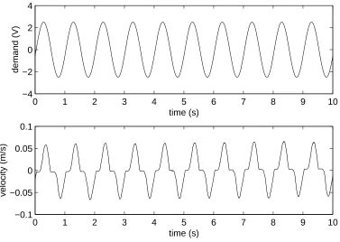
Figure 2: Experimental results showing the velocity deadzone behavior exhibited by the plant; (a) open-loop
demand and (b) velocity response.
of the table is measured using a linear potentiometer.
At low frequencies the velocity of the plant exhibits behaviour which closely replicates a deadzone
nonlin-earity. Where, theoretically, an ideal deadzone nonlinearity is defined as:
vo= 0 for |vi|< vc,
vo=vi−vc for vi≥vc,
vo=vi+vc for vi≤ −vc,
(10)
wherevi is the input,vo is the output andvc is the deadzone offset. Experimentally, the deadzone behaviour
is demonstrated in Figure 2, for the case where a sinusoidal, 1Hz, 2.5V amplitude, open-loop input (Figure 2
(a)) is applied to the plant. The velocity response, Figure 2 (b), clearly exhibits regions of zero velocity lasting
around 0.1s every time the direction of travel changes, which may be approximated as a deadzone nonlinearity.
For this plant, it is thought that the deadzone is caused by a combination of the power amplifier dynamics and
stiction in the motor and linear bearing.
A first-order MRAC strategy is used to control the displacement of the moving table. It is worth noting that
with the minimization of the nonlinear plant behavior. This is because with velocity control the magnitude of
both the demand velocity,r, and the feedback velocity,x, are small, assuming that (as would normally be the
case) the demand frequency is lower than the reference model break frequency. Therefore the rate of change in
the controller gains are small over the region where non-linear behavior occurs. Conversely, with displacement
control, the non-linear regions coincide with the regions of large amplitude displacementsxandrand therefore
rapid gain adaption can occur over the non-linear regions, giving more responsive control.
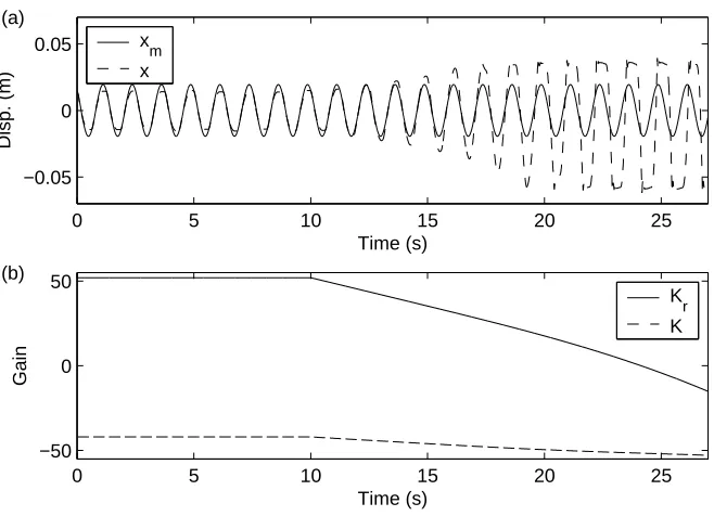
Figures 3 (a) and (b) show the plant displacementxcompared with the reference model outputxmand the
system gains respectively when the plant displacement is controlled using the MRAC algorithm. The reference
model parameters used weream=bm= 40 and the demand was a 0.02m amplitude, 0.8Hz sinusoid. Initially
the gains are set toKr0= 52 andK0=−42 which were found to give reasonably smooth linear control. Over
the first 10s of the test the adaptive gain weightingsαandβwere set to zero, i.e. a constant gain linear control
strategy was used. It can be seen that over this period of time the table response was reasonably good except
over the non-linear velocity deadzone regions where there is a marked error between the table displacement
and the reference model output. Att= 10s the unmodified adaptive MRAC strategy was activated by setting
non-zero adaptive gain weightings (α= 10 andβ = 1). It can be seen that with the adaptive control strategy
the gains rapidly changed (in this case winding down) resulting in very poor displacement control, and within
6 oscillations at 18.5s the maximum positive travel of the table was exceeded. This type of stability loss was
observed with lower adaptive gain weightings over an extended time frame and has been observed in other
nonsmooth systems [11]. The mechanism behind this type of stability loss is considered next.
3.2
Localized analysis of the MRAC algorithm
In this section the error equation (Equation (7)) developed in Section 2 is reformulated as a nonlinear dynamical
system. Using a dynamical systems approach the system stability can be analyzed using local analysis close to
the equilibrium points. The plant and MRAC algorithm is assumed to be a dynamical system of the form
˙
ξ=f(ξ, t), (11)
whereξ={xe, K, Kr}T is the state vector.
repre-0 5 10 15 20 25 −0.05
0 0.05
Time (s)
Disp. (m)
(a)
0 5 10 15 20 25
−50 0 50
Time (s)
Gain
(b)
x m x
[image:9.595.141.470.111.349.2]K r K
Figure 3: Displacement control of the experimental plant using the standard unmodified MRAC algorithm,
initially using linear gains (α = β = 0) with adaptive gain weighting set to α= 10, β = 1 at t = 10s; (a)
displacement response and (b) system gains.
sentation of the plant and MRAC algorithm may be expressed as
˙
xe = −amxe+b KE−K(xm−xe) +b KrE−Krr
˙
K = α xexm−x2e
+β
xex˙m+ (xm−2xe)−amxe+b KE−K(xm−xe) +b KrE−Krr
˙
Kr = αxer+βxer˙+r−amxe+b KE−K(xm−xe) +b KrE−Krr ,
(12)
where the parametersam,b,αandβ are constant and the parametersr, ˙r,xmand ˙xmare time varying input
signals (see Appendix A1 for a formulation using the variables (KE−K) and (KE
r −Kr) in place ofK and
Kr).
The first step is to find the equilibrium points of Equation (12). Having done this the stability of each
equilibrium point can be examined using local analysis of the linearized system. To find the equilibrium points
for the system we need to solve the equation: f( ˜ξ, t) = 0, where ( ˜ ) indicates an equilibrium point. By
inspection, two conditions are necessary for the system to be at equilibrium
˜
xe= 0, (13)
from which it can be seen that there are an infinite number of ˜K, and corresponding ˜Kr, values which give
f( ˜ξ, t) = 0.
Defining a subset of the complete system state space as Σ ={xe×K×Kr∈R3}, then Equations (13) and
(14) define the equilibrium manifold (denoted Γ) which represents the set of equilibrium points ˜ξ={0,K,˜ K˜r}T.
In the case of ˙r= ˙xm= 0 andxm/rconstant (this is the case for a steady state unit step input) the manifold
representing the equilibrium solutions in Σ defined by Equation (14) is a straight line in theK, Krplane. The
projection of the dynamics onto Γ for the step input case is shown in Appendix A2.
In general, however,randxmare time varying (with the relationship betweenxmandrbeing governed by
Equation (3). Equation (14) will be satisfied regardless of xm andrif ˜K=KE and ˜Kr=KrE corresponding
to the equilibrium point at ˆξE={0, KE, KrE}T. In addition to this time invariant point, there are an infinite
number of time dependent solutions to Equation (14) which require time varying ˜K and ˜Kr for time varying
xmandr. However, from Equations (12) it can be observed that for ˜K and ˜Kr to vary with time the errorxe
must be non-zero. Therefore at equilibrium points other than ˜ξE ={0, KE, KrE}T, limit cycle type behavior
exists which oscillate around Γ. The existence of oscillations in the gain can also indicate factors such as
under-modeling of the plant.
To analyze the local stability of the system near an equilibrium points ˜ξ, the right hand side of Equation
(11) is expanded as a Taylor series at ˜ξ, from which the linear approximation to the system is
˙
ξ≈Dfξ( ˆξ)(ξ−ξˆ), (15)
whereDfξ( ˆξ) is the Jacobian Matrix evaluated at an equilibrium pointξ= ˆξ,f( ˜ξ) = 0, and all theO((ξ−ξ˜)2)
and higher terms have been neglected. The stability of the local dynamics is given by the eigenvalues ofDfξ( ˜ξ).
Using Equation (12), the Jacobian for the system at an equilibrium point ˜ξis found to be
Dfξ( ˜ξ) =
−am−b(KE−K˜) −bxm −br
αxm−β[amxm+b(KE−K˜)xm−x˙m] −βbx2m −βbrxm
αr−β[amr+b(KE−K˜)r−r˙] −βbxmr −βbr2
This Jacobian has three eigenvalues,λ1= 0 and
λ2,3=− 1
2[am+b(K
E−K˜) +βb(x2 m+r
2 )]±1
2S, (17)
where S2
= [am+b(KE−K˜) +βb(x2m+r 2
)]2
−4b[α(x2 m+r
2
) +β(xmx˙m+rr˙)]. It should emphasized at
this point that λ1 is time invariant, and indicates neutral (i.e. non-asymptotic) stability in the eigenvector
direction which is given by
e1= [0,−r/xm,1]T. (18)
In this case the eigenvector,e1 is always tangent to the exact matching manifold, Γ.
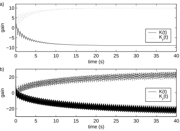
Figure 4 (a) shows the adaptive gains for a simulation of first-order plant controlled using the unmodified
MRAC strategy. The initial gains were set to zero, and the adaptive weightings whereα= 1000 andβ= 100.
The plant and reference model parameters used werea=b= 4 andam=bm= 40 respectively and the demand
rwas a 1V amplitude 1Hz sinusoid. It can be seen that the gains settle to the Erzberger values of KE =−9
andKE
r = 10 in around 20 seconds. However if noise disturbance is added to the plant output, gain wind-up
can occur as shown in Figure 4 (b), where a 50Hz 0.1V sinusoid is added to the plant output. Yang [25] shows
that the neutral localized stability in the direction of the equilibrium manifold leads to gain wind-up when a
system is subjected to noise and that the wind-up occurs along the manifold (Γ) i.e. in the direction of±e1,
depending on system parameters and input signals.
4
The modified MRAC algorithm
To alleviate the problem of gain wind-up, a method is presented for replacing the undesirable zero eigenvalue
with a constant (real) negative eigenvalue. This is achieved by replacing the time varying adaptive gains K
andKrwith new modified gains, Km andKrm respectively, resulting in the control equation
u(t) =Km(t)x(t) +Krm(t)r(t) (19)
The modified gains are calculated using the equations
Km=
s s+ρ2K+
ρ2
s+ρ2K
∗ (20)
Krm=
s
s+ρ2Kr+
ρ2
s+ρ2K ∗
0 5 10 15 20 25 30 35 40 −10
−5 0 5 10
time (s)
gain
a)
K(t) K
r(t)
0 5 10 15 20 25 30 35 40
−20 0 20
time (s)
gain
b)
[image:12.595.118.488.110.379.2]K(t) Kr(t)
Figure 4: Simulation of a plant controlled using the MRAC algorithm, a) with no noise and b) with noise
added to the plant output, using plant parametersa=b= 4 and reference model parametersam=bm= 40.
where s is the Laplace transform variable, ρ is a constant and K∗ and K∗
r are gain constants. A condition
on the values of these gain constants is derived in the subsequent analysis. Similar gain “leakage” strategies,
have been applied to an integral only adaptive gain strategy, i.e. a MRAC controller with β= 0 — these are
discussed in [14]. It can be seen from equations 20 and 21 that the modified gainsKmandKrmare generated
using two signals filtered by first-order transfer functions - a high-pass first-order filter applied to K or Kr
respectively and a low-pass first-order filter applied toK∗or K∗
4.1
Dynamics of the modified algorithm
By considering the localized stability of the modified system it can be shown that all three system eigenvalues
are stable. The error dynamics for the modified system may be expressed as
˙
xe = −amxe+b KE−Km(xm−xe) +b KrE−Krmr
˙
Km = α xexm−x2e
+β
xex˙m+ (xm−2xe)−amxe+b KE−Km(xm−xe) +b KrE−Krmr
+ρ2
(K∗−K m)
˙
Krm = αxer+β
xer˙+r
−amxe+b KE−Km
(xm−xe) +b KrE−Krm
r +ρ2 (K∗
r−Krm), (22)
By inspection, there are now four conditions that are necessary for the system to be at equilibrium:
˜
xe= 0 (23)
(KE−K˜
m)xm+ (KrE−K˜rm)r= 0 (24)
˜
Km=K∗ (25)
˜
Krm=Kr∗ (26)
Note that ifρ= 0 we revert to the unmodified case where only the first two conditions are required.
For these four conditions (23)–(26) to be satisfied it follows that, sincexmandrare time varying,K∗=KE
and K∗
r =KrE and that equilibrium only exists at a single point, ˜ξE ={0, KE, KrE}T. In Section 3 it was shown that with the standard MRAC strategy there exists a manifold of equilibrium points (Γ), and that
the Jacobian of each equilibrium point had a zero eigenvalue. For the modified algorithm the manifold of
equilibrium points has been reduced to a single point, and computing the Jacobian matrix reveals that the
time invariant eigenvalue now takes the valueλ1=−ρ 2
in the eigenvector directione1= [0,−r/xm,1]T.
Therefore the modification to the MRAC algorithm has eliminated the neutral (i.e. non-asymptotic)
local-ized stability. However, to implement the controller, knowledge on the Erzberger gains are needed to selectK∗
and K∗
r. In practice these gain values will not be known accurately but can be estimated from a first-order
transfer function approximation to the plant dynamics. Errors in the estimation of the Erzberger gains used
for settingK∗ andK∗
r will cause oscillations in the gains about theK∗ andKr∗ values. This is demonstrated
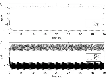
in simulation in Figure 5 (a) whereK∗=−10 andK∗
0 5 10 15 20 25 30 35 40 −10
−5 0 5 10
time (s)
gain
a)
K(t) K
r(t)
0 5 10 15 20 25 30 35 40
−10 0 10
gain
time (s) b)
[image:14.595.118.487.104.380.2]K(t) Kr(t)
Figure 5: Simulation of a plant controlled using the modified MRAC algorithm, a) with no noise and b)
with noise added to the plant output, using plant parameters a = b = 4 and reference model parameters
am=bm= 40. Note the gain oscillations which occur in (a) are due toK∗6=KE andKr∗6=KrE.
plant output, Figure 5 (b), it can be seen that the modified control algorithm has eliminated the gain wind-up.
One possible method for overcoming the need for setting K∗ and K∗
r values based on estimates of the
Erzberger gains is to start controlling the plant using the standard MRAC algorithm (i.e.ρ= 0). Then as the
gains adapt, the modification could be activated, at sayt=tρ, by setting a non-zeroρvalue and setting K∗
and K∗
r values to the current gain values, K(tρ) and Kr(tρ) respectively. However, for the plant considered
in this paper the standard MRAC algorithm was insufficiently stable for this method to be practical. Instead
theK∗ andK∗
r gains were set to the gain values that were found to provide good linear (fixed-gain) control,
4.2
Experimental implementation
For the moving table, it has already been shown, in Figure 3 that when the standard MRAC strategy is used
gain wind-up occurs which leads to system instability. Using the modified algorithm, Figures 6 (a), (b) and
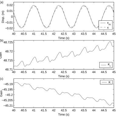
(c) show the displacement response and the system gains Kr and K respectively for the case where ρ= 10,
α= 2000,β = 200, K∗
r = 52 andK∗ =−42. The traces are shown after 40s of adaption, and it can be seen that with this modified MRAC strategy the control is significantly better than the linear control shown in the
first 10s of Figure 3. In this case there is only a limited deterioration of the control accuracy over the velocity
deadzone regions. Note also that the unmodified MRAC approach, shown after 10s in Figure 3, could not
control this plant at all.
Figures 6 (b) and (c) show how the gains adapt in a regular oscillatory pattern at twice the frequency of
the demand. It is interesting to note that the gains also exhibit a very slight gain wind-up. The analysis in
the previous section suggested that with the modified algorithm no gain wind-up would occur. However, this
analysis was based on the dynamics of the plant being approximated to a first-order linear system. There are
two contributing factors for the small amount of gain wind-up observed in the experiments; (i) The gains have
not yet fully adapted to the final values. Simulations of the modified algorithm indicate that ifK∗6=KE and
K∗
r 6=KrE that there is a very slow movement of trajectories in Σ towards the single fixed point, ˜ξE. (ii) There is significant under-modeling of the plant dynamics. In this case the plant dynamics may be more accurately
modelled as second order than as first order. Also the nonsmooth discontinuity in the plant is not included in
the analysis of section 3.2.
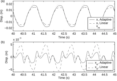
We have used a modified version of the MRAC algorithm to successfully control a plant with a nonlinear
deadzone. To assess the effectiveness of such a controller it is worth examining the control of the plant when
using the linear equivalent to the MRAC algorithm, i.e. the MRAC controller with adaptive weightingsαand
β set to zero. Figures 7 (a) and (b) show comparisons of the table performance using the modified MRAC
algorithm and the linear equivalent to the adaptive MRAC strategy. The fixed gains in the linear controller
take the same values as the modified MRACK∗
r andK∗gains. Figure 7 (a) shows the displacement response
using the linear and the adaptive modified MRAC controllers compared to the reference model displacement
xm. It can be seen that the performance of the modified MRAC strategy is better than that of the linear
40 40.5 41 41.5 42 42.5 43 43.5 44 44.5 45 −0.02
−0.01 0 0.01 0.02
Disp. (m)
Time (s) (a)
40 40.5 41 41.5 42 42.5 43 43.5 44 44.5 45 48.71
48.715 48.72 48.725
Gain
Time (s) (b)
40 40.5 41 41.5 42 42.5 43 43.5 44 44.5 45 −45.21
−45.205 −45.2 −45.195 −45.19
Gain
Time (s) (c)
x
m
x
Kr
[image:16.595.114.496.220.608.2]K
Figure 6: Experimental results showing displacement control of the plant using the modified MRAC algorithm;
40 40.5 41 41.5 42 42.5 43 43.5 44 44.5 45 −0.02
−0.01 0 0.01 0.02
Disp. (m)
Time (s) (a)
40 40.5 41 41.5 42 42.5 43 43.5 44 44.5 45 −5
0 5
x 10−3
Time (s)
Disp. (m)
(b)
x, Adaptive x, Linear xm
xe, Adaptive x
[image:17.595.114.494.117.381.2]e, Linear
Figure 7: Experimental results showing displacement control of the plant using the linear equivalent to the
MRAC algorithm; (a) displacement response and (b) system errorxm−x.
strategies are shown in Figure 7 (b), where the modified adaptive error is approximately half the maximum
amplitude of that of the linear control.
5
Conclusions
In this paper a modified MRAC controller has been presented which has been applied to a nonsmooth plant.
The phenomena of gain wind-up, which commonly occurs in MRAC control systems, has been analyzed using
localized stability analysis. Using this analysis the inherent zero eigenvalue which exists in the unmodified
system, is seen to be the major cause of gain wind-up in the presence of plant uncertainties such as a nonsmooth
discontinuities. A modification to the MRAC strategy has been proposed to eliminate the zero eigenvalue and
reduce the infinite manifold of equilibrium solutions, Γ, to a single equilibrium point, ˜ξE. Simulations of a
plant with first order dynamics have been used to demonstrate the presence of gain wind-up when the plant
output is subjected to a noise disturbance in the unmodified MRAC. However, with the modification to the
Experimental testing of the MRAC strategy was performed on a small-scale motor-driven moving table in
displacement control. The table dynamics are nonsmooth, with the velocity response exhibiting a large
dead-zone nonlinearity. Initially tests were conducted on a linear equivalent to the MRAC strategy (i.e. equivalent
to setting the MRAC adaptive gain weightings to zero). With tuning, the linear controller performed
reason-ably well. However when the gains were allowed to adapt, using the standard unmodified MRAC strategy,
the control performance was very poor, to the extent that it was impossible to get the unmodified MRAC to
stabilize. The control of the table using the modified MRAC strategy was a significant improvement both on
the linear control and the unmodified MRAC. The modified MRAC, had approximately half the maximum
dis-placement error than when the linear controller was used. The gains oscillations observed in the experimental
results occurred at twice the frequency of the demand signal with a slight gain wind-up. This wind-up can be
attributed to continued gain evolution at a slow rate and under-modeling of the plant dynamics.
In the future, it is anticipated that further refinement of the modified MRAC algorithm will be possible.
In particular, it would be beneficial forK∗ andK∗
r to be optimised on-line to minimise the oscillations inKm
and Krm, as was observed in the simulation results due to errors in matching K∗ and Kr∗ to KE and KrE
respectively. In addition to this, a systematic technique for selecting the optimal value ofrhofor a particular
plant would be a highly desirable research objective. The improvement in robustness which can be achieved
by the modifications demonstrated in this work may also lead to this type of algorithm being applicable to a
wider range of practical applications.
6
Acknowledgements
Lin Yang would like to acknowledge the support of the Dorothy Hodgkin Postgraduate Award scheme. The
authors would also like to acknowledge the support of the EPSRC. David Virden is supported by research
grant GR/R99539/01 and David Wagg by an Advanced Research Fellowship.
Appendix
In appendix A1 we outline the background material on the derivation of MRAC for systems of higher order
be obtained for the global dynamics along Γ.
A1
Higher-order MRAC formulations
For the linear state space system in the form ˙x(t) =Ax(t) +Bu(t), wherexis then×1 state variable vector,
uis them×1 control signal vector,Ais an×nmatrix representing the linear dynamics of the plant, andBis
a n×mmatrix. The controller is given by u(t) =K(t)x(t) +Kr(t)r(t), wherer(t) is the reference (demand)
signal, K(t) is the feedback adaptive gain and Kr(t) the feed forward adaptive gain [13–15]. All the input
signals we use in this work are at least persistently exciting to order one [14]. Substituting forugives
˙
x=Ax+B(Kx+Krr) = (A+BK)x+BKrr. (27)
The plant is now controlled to follow the output from a reference model with known dynamics ˙xm(t) =
Amxm(t)+Bmr(t), wherexmis the state of the reference model andAmandBmare linear reference equivalents
ofAandB [12]. The system error dynamics are now
˙
xe=Amxe+ (Am−A−BK)x+ (Bm−BKr)r, (28)
and for exact matchingA+BKE =A
mandBKrE =Bm. Assuming all matrix (pseudo) inverses exist we can
obtain expressions (the Erzberger conditions [15]) for the gain values asKE =B†(A
m−A) andKrE=B†Bm, where ()† denotes the pseudo-inverse and ()E denotes the constant Erzberger gain value. The Erzberger gains
can be used to express the matrix terms given in Equation (28), as
˙
xe=Amxe+BΦTw (29)
where Φ = (KE −k), k = {K, K
r}T,KE = {KE, KrE}T and w(t) = {x, r}T and we assume that B has a pseudo-inverse such thatBB† =I. The adaptive gains are defined in a proportional plus integral formulation
k=α
Z t
0
yew(τ)dτ+βyew(t). (30)
whereαandβ are control weightings representing the adaptive effort, andye=CexewhereCecan be chosen
to ensure the stability of the feed forward block [12].
If we let φ(t) = (KE−K(t)) and ψ(t) = (KE
r −Kr(t)), then Φ(t) ={φ, ψ}T and ξ={xe, φ, ψ}T is the state vector. By using the fact the KE is a constant, ˙Φ = −k˙, and by using Equation (30) we can obtain
Applying this formulation to the first order plant/controller system described in 2 gives the following system
of ODE’s (assumingCeis incorporated intoαandβ)
˙
xe=−amxe+b[φ(xm−xe) +ψr],
˙
φ=−αxe(xm−xe)−β[(−amxe+b[φ(xm−xe) +ψr])(xm−2xe) +xex˙m],
˙
ψ=−αxer−β((−amxe+b[φ(xm−xe) +ψr])r+xer˙).
(31)
In this formulation ˜ξE={0,0,0}.
A2
Global dynamics along
Γ
Using Equation (31) we can define a subset of the complete state space ˆΣ ={R×R×R: (xe, φ, ψ)}. Then
by defining a transformation matrixT = [e1, e2, e3], consisting of the eigenvectors of the linearized system, the
transformationξ=T ν can be made whereν = [u, v, w]. Rewriting Equation (31) in the form ˙ξ=Lξ+h(ξ),
whereLis the linear part andh(ξ) the nonlinear part, gives an expression for the dynamics in the transformed
coordinates ˙ u ˙ v ˙ w
=T−1
LT u v w
+T−1
h(ξ). (32)
In this coordinate set, ˙urepresents the dynamics along the exact matching manifold, Γ, andT−1
LT has the
following block diagonal structure
T−1
LT =
0 ... 0 0
. . . .
0 ... s12 s12
0 ... s21 s22 (33)
where sij represents an unspecified algebraic term. Now T−1LT is in a block diagonal form as discussed
by [20] in relation to center manifolds. In effect the dynamics associated with the zero eigenvalue — the
leading diagonal term inT−1
LT — have been linearly decoupled from the dynamics associated with the stable
eigenvalues — represented by the block formed by the sij, i, j = 1,2 terms. However, unlike the classical
approach to center manifold theory for the systems described by [20, 29], the adaptive system has a time
onto Γ, and for a step input, Γ is a linear time invariant manifold. Therefore Γ is the center manifold in the
system. A similar type of center manifold analysis has been carried out for a different class of adaptive systems
by [21]. As pointed out by [21], decoupling the center manifold dynamics allows us to ignore the remaining
system dynamics.
The dynamics along Γ can be extracted from Equation (32) as the first row of T−1
multiplied by the
nonlinear vectorh(ν).
˙
u= [T−1 11 , T−
1 12 , T−
1 13 ]
h1(ξ)
h2(ξ)
h3(ξ) (34)
The form of Equation (34) will then enable us to determine the dynamics along Γ. For the step input case, the
matrix of linear terms is
L=
−am b b
−α+βam −βb −βb
−α+βam −βb −βb (35)
and the nonlinear vector
h(ξ) =
−bφxe
−αx2
e−β[2amx2e−3bφxe+ 2bφx2e−2bψxe]
βbφxe (36)
The transformation matrix,T has the form
T =
0 λˆ2/χ ˆλ3/χ
−1 1 1
1 1 1
(37)
where ˆλi=λi+ 4βb,i= 1,2 andχ= (βam+bφβ˜ −α). The inverse transform matrix is then given by
T−1 = 0 1 2 − 1 2
−ˆ χ λ3−ˆλ2
1 2
ˆ λ3
ˆ λ3−ˆλ2
1 2
ˆ λ3
ˆ λ3−ˆλ2
χ ˆ
λ3−ˆλ2 −
1 2
ˆ λ2
ˆ
λ3−ˆλ2 −
1 2
ˆ λ2
ˆ λ3−λˆ2
(38) such that ˙
u=1
2h2(ξ)− 1
substituting forhgives
˙
u=βb(φ+ψ)xe−(
α
2 +β(am+bφ))x 2
e. (40)
Then from the relationξ=T ν
xe= λχ2v+λχ3w
φ=−u+v+w
ψ=u+v+w
(41)
so that we can obtain an expression for the dynamics along Γ in terms of the coordinate setν,
˙
u = 2βb(v + w)(λˆ2
χv +
ˆ
λ3
χw) − ( α
2 + β(am + b(−u + v + w)))( ˆ
λ2
χv +
ˆ
λ3
χw)
2
. (42)
From equation (40) , if xe 6= 0 then ˙u will have some value which represents the rate of change of the
coordinate along (i.e. tangent to) the exact matching manifold, Γ.
References
[1] Qammar, H. K., and Mossayebi, F., ‘System identification and model based control of a chaotic system’,
International Journal of Bifurcation and Chaos4(4), 1994, 843–851.
[2] Petrov, V., Crowley, M. F., and Showalter, K., ‘An adaptive control algorithm for tracking unstable
periodic orbits’, International Journal of Bifurcation and Chaos4(5), 1994, 1311–1317.
[3] Wu, C. W., Yang, T., and Chua, L. O., ‘On adaptive synchronization and control of nonlinear dynamical
systems’, International Journal of Bifurcation and Chaos6(3), 1996, 455–471.
[4] Stoten, D. P., and Di Bernardo, M., ‘Application of the minimal control synthesis algorithm to the control
and synchronization of chaotic systems’, International Journal of Control65(6), 1996, 925–938.
[5] Dong, X., Chen, G., and Chen, L., ‘Adaptive control of the uncertain duffing oscillator’, International
Journal of Bifurcation and Chaos7(7), 1997, 1651–1658.
[6] Di Bernardo, M., ‘An adaptive approach to the control and synchronization of continuous-time chaotic
[7] Di Bernardo, M., Adaptive control and analysis of nonlinear chaotic dynamical systems, PhD thesis,
University of Bristol, 1998.
[8] Wagg, D. J,. ‘Adaptive control of nonlinear dynamical systems using a model reference approach’.
Mec-canica38, 2003, 227–238.
[9] de la Sen, M., ‘Lyapunov stability and adaptive regulation of a class of nonlinear nonautonomous
second-order differential equations’, Nonlinear Dynamics28, 2002, 261–272.
[10] Ioannou, P. A., and Kokotovic, P. V., ‘Instability analysis and improvement of robustness of adaptive
control’, Automatica20(5), 1984, 583–594.
[11] Virden, D., and Wagg, D. J., ‘System identification of a mechanical system with impacts using model
reference adaptive control’,Proc. IMechE. Pat I: Journal of Systems and Control Engineering219, 2005,
121–132.
[12] Landau, Y. D., Adaptive control:The model reference approach, Marcel Dekker, New York, 1979.
[13] Sastry, S., and Bodson, M., Adaptive control:Stability, convergence and robustness, Prentice-Hall, New
Jersey, 1989.
[14] ˚Astr¨om, K. J., and Wittenmark, B., Adaptive Control, Addison Wesley, 1995.
[15] Khalil, H. K., Nonlinear Systems, Macmillan, New York, 1992.
[16] Mareels, I. M. Y., and Bitmead, R. R., ‘Bifurcation effects in robust adaptive control’,IEEE Transactions
on Circuits and Systems35(7), 1988, 835–841.
[17] Huberman, B. A., and Lumer, E., ‘Dynamics of adaptive systems’, IEEE Transactions on Circuts and
Systems37(4), 1990, 547–550.
[18] Gonzalez, G. A., ‘Dynamical behaviour arising in the adaptive control of the generalized logistic map’,
Chaos, Solitions and Fractals8(9), 1997, 1485–1488.
[19] Townley, S., ‘An example of a globally stabilizing adaptive controller with a generically destabilising
[20] Guckenheimer, J., and Holmes, P., Nonlinear oscillations, dynamical systems, and bifurcations of vector
fields, Springer-Verlag, New York, 1983.
[21] Leach, J. A., Triantafillidis, S., Owens, D. H., and Townley, S., ‘The dynamics of universal adaptive
stabilization: computational and analytical studies’, Control-Theory and Advanced Technology 10(4),
1995, 1689–1716.
[22] Gu, E.Y.L., ‘Dynamic systems analysis and control based on a configuration manifold model’, Nonlinear
Dynamics19, 2000, 113–134.
[23] Townley, S., ‘Topological aspects of universal adaptive stabolization’, SIAM Journal of Control and
Optimization34(3), 1996, 1044–1070.
[24] Ronki Lamooki, G. R., Townley, S., and Osinga, H. M., ‘Normal forms, bifurcations and limit dynamics
in adaptive control systems’, International Journal of Bifurcation and Chaos15(5), 2005, 1641–1664.
[25] Yang, L.,A modified model reference adaptive control algorithm to improve system robustness, MSc Thesis,
University of Bristol, 2004.
[26] Vinagre, B.M., Petr´a, I., Podlubny, I., and Chen, Y.Q., ‘Using fractional order adjustment rules and
fractional order reference models in model-reference adaptive control’, Nonlinear Dynamics 29, 2002,
269–279.
[27] Rey, G. J., Johnson J, R., and Dasgupta, S., ‘On tuning leakage for performance-robust adaptive-control’,
IEEE Transactions on Automatic Control34(10), 1989, 1068–1071.
[28] Nascimento, V. H., and Sayed, A. H., ‘Unbiased and stable leakage-based adaptive filters’, IEEE
Transactions on Signal Processing47(12), 1999, 3261–3276.