7. Syntax
In syntactic research, it is important to distinguish between judgments that bear on
grammaticality and those that bear on semantic anomaly. For example, though it is syntactically well-formed, and thus grammatical, the phrase colorless green ideas is semantically anomalous. Table 7.1 illustrates the distinction between grammaticality judgments and semantic anomaly judgments.
Table 7.1. Illustration of the difference between grammaticality and semantic anomaly.
colorless ideas green colorless green ideas
semantically anomalous
subversive ideas communist subversive communist ideas
semantically well-formed
grammatically ill-formed grammatically well-formed
However, the grammaticality/anomaly distinction is over-simple. For example, with the appropriate discourse context leading up to it the apparently anomalous colorless green ideas can be judged as semantically well-formed. Similarly, when a phrase is grammatically ill-formed like subversive ideas communist is given an appropriate context, it isn’t clear that it actually has a compositional semantic interpretation. Nonetheless, the distinction between grammaticality and anomaly is central to any discussion of syntactic theory.
I bring this up because recently researchers have been turning to naive speakers for syntactic data (Bard et al., 1996; Schütze,1996; Cowart, 1997; Keller, 2000, and many others). The problem is that naive speakers can’t tell you that colorless green ideas is syntactically OK but semantically odd. They just think it isn’t nearly as natural, or acceptable, as subversive communist ideas. So, to use data given by naive speakers we have to devote a good deal more effort to acquiring
syntactic data, and still there are likely to be concerns that we don’t actually know why a person judged one phrase to be relatively unacceptable while another is perfectly fine.
is happening is that the budding linguist is developing the distinction between grammaticality and anomaly, but it seems just as likely that we are learning to have stronger opinions or intuitions about grammaticality than nonlinguists. The possibility that the “data” are infected with the researcher’s expectations is a fundamental concern that appears to be driving the push to get syntactic data from naive speakers (see Inton-Peterson, 1983; and Goldinger & Azumi, 2003 for evidence that expectations can color the results even in “low level” tasks).
The second good reason to bother getting data from naive speakers has to do with sampling theory. If we want to say things about English syntax, for example, then we need to get data from a representative sample of the population of people who speak English (of some variety).
I don’t think that there is much disagreement about these problems with using linguists’ intuitions as the data base for syntactic theory, but there has to be a viable alternative. One of the most serious concerns about “experimental” or “empirical” alternatives has to do with whether information about grammaticality can be gleaned from naive speakers’ acceptability judgments. Consider table 7.1 again. If we collect acceptability judgments for items in all four cells of the table we can distinguish, to a certain degree, between judgments that are responsive primarily to semantic anomaly (the rows in the table) from judgments that are responsive to grammaticality. Here we are using a hypothesis testing approach, in which we hypothesize that these utterances differ in the ways indicated in the table on the basis of our linguistically
sophisticated judgments.
7.1 Measuring sentence acceptability
In syntax research an interval scale of grammaticality is commonly used. Sentences are rated as grammatical, questionable (?, or ??), and ungrammatical (*, or **). This is essentially a 5-point category rating scale, and we could give people this rating scale and average the results, where ** = 5, * = 4, ?? = 3, ? = 2, and ø = 1. However, it has been observed in the study of sensory impressions (Stevens, 1975) that raters are more consistent with an open-ended ratio scale than they are with category rating scales. So, in recent years, methods from the study of
psychophysics (subjective impressions of physical properties of stimuli) have been adapted in the study of sentence acceptability.
scale, there is no guarantee that the interval between * and ** represents the same difference of impression as ? and ??. Magnitude estimation provides judgments on an interval scale for which averages and standard deviations can be more legitimately used. Third, categorical scaling limits our ability to compare results across experiments. The range of acceptability for a set of
sentences has to be fit to the scale, so what counts as ?? for one set of sentences may be quite different than what counts as ?? for another set of sentences. You’ll notice that I’ve employed a set of instructions (Appendix A) that imposes a similar range on the magnitude estimation scale. I did this by giving a “modulus” phrase and instructed the raters to think of this as being an example of a score of 50. I did this to reduce the variability in the raters’ responses, but it put the results onto an experiment-internal scale so that the absolute values given by these raters cannot be compared to the ratings given in other experiments that use different instructions with a different modulus phrase.
In sum, magnitude estimation avoids some serious limitations of category scaling. But what exactly is magnitude estimation? The best way I know to explain it is by way of demonstration, so we’ll work through an example of magnitude estimation in the next section.
7.2 A psychogrammatical law?
Keller (2003) proposes a psychogrammatical law relating the number of word order constraint violations and the perceived acceptability of the sentence, using magnitude estimation to estimate sentence acceptability. The relationship can be expressed as a power function:
€
R
=
kN
vp A syntactic power law.Where R is the raters’ estimation of sentence acceptability and Nv is the number of constraint violations in the sentence being judged, p is exponent of the power function and k is a scale factor. Note that this relationship can also be written as a simple linear equation using the log values of Nv and R.
€
log
R
=
log
k
+
p
log
N
v Expressed as a linear regression equation.The exponent (p) in Keller’s power law formulation for the relationship between acceptability and constraint violations was 0.36.
Hetzron (1978) proposed a word order template for prenominal adjectives in English (Table 7.2) that putatively follows universal constraints having to do with semantic or pragmatic properties of adjectives, but apparently the best predictions of adjective ordering in English corpora come from considerations of language-specific and often adjective-specific conventions rather than universal principles (Malouf, 2000). Nonetheless, Hetzron’s template accounts for at least some portion of the prenominal adjective order patterns found in spoken English (Wulff, 2003).
So we will use Hetzron’s word order template to make predictions about acceptability, in search of a psychogrammatical law similar to the one Keller suggested. In Hetzron’s template, position 0 is the head noun of the phrase and prenominal adjectives in a noun phrase typically come in the order shown in table 7.2 (with some of these categories being mutually exclusive).
Table 7.2 The Hetzron (1978) template of prenominal adjective order.
13 epistemic qualifier “famous”
12 evaluation* “good”, “bad”, “nice” 11 static permanent property* “wide”, “tall”, “big” 10 sensory contact property “sweet”, “rough”, “cold”
9 speed “fast”, “slow”
8 social property “cheap”
7 age* “young”, “new”, “old”
6 shape “round”, “square”
5 color* “blue”, “red”, “orange”
4 physical defect “deaf”, “chipped”, “dented”
3 origin* “Asian”, “French”
2 composition* “woolen”, “silk”, “steel”
1 purpose “ironing”
0 NOUN
* I used these in the experiment.
The hypothesis that I wish to test is that placing adjectives in the “wrong” order will result in a greater decrease in acceptability if the adjectives are from categories that are further apart from each other on this scale. This predicts that “woolen nice hat” (transposing adjectives from category 12 and 2) is worse than “woolen Asian hat” (categories 2 and 3). In some cases this seems intuitively to be true, in others it may not be quite right. An empirical study is called for.
[12]attitude = ("good","nice","pleasant","fun","tremendous","wonderful","intelligent"); [11]size = ("big","tall","small","large","tiny","huge","wide","narrow","short");
[7]age = ("old","young","new");
[5]color = ("black","white","red","blue","pink","orange");
[3]origin = ("French","Dutch","English","Asian","Irish","Turkish"); [2]material = ("steel","woolen","wooden","lead","fabric");
[0]noun = ("hat","plate","knob","wheel","frame","sock","book","sign","dish","box","chair", "car","ball");
Phrases were then generated by selecting randomly from these sets to form phrases with differing degrees of separation along the template. Random generation of phrases produces some that are semantically anomalous (“pleasant Asian sock”) and others that are semantically fine (“old pink plate”). I used different randomly generated lists for each participant in order to provide a rough control for the effects of semantic anomaly, because the results were then averaged over
semantically anomalous and non-anomalous phrases. However, a more careful control would have not left the factor of semantic anomaly to chance, instead controlling anomaly explicitly on the basis of a pretest to insure that either no anomalous phrases were used or that each participant saw a fixed number of anomalous and non-anomalous phrases.
There were four types of stimuli involving adjectives at four different degrees of difference on the Hetzron template. The group 1 pairs of adjectives come from slots that are close to each other on the template, while the group 4 pairs come from distant slots. If the template distance hypothesis is on the right track, group 4 order reversals will be less acceptable than group 1 order reversals.
Table 7.3 Adjective order template distance of the four groups of phrases used in the experiment. “Template distance” is the difference between the indices in the Hetzron template of the two adjectives in the phrase.
Group 1
attitude, size 12-11 = 1
size, age 11-7 = 4 average distance = 2 age, color 7-5 = 2
origin, color 3-2 = 1
Group 2
attitude, age 12 - 7 = 5
age, origin 7 - 3 = 4 color, material 5 - 2 = 3
Group 3
attitude, color 12 - 5 = 7
size, origin 11 - 3 = 8 average distance = 6.33 age, material 7 - 2 = 5
Group 4
attitude, origin 12 - 3 = 9 average distance = 9 size, material 11 - 2 = 9
[image:6.612.140.510.80.272.2]The experiment (appendix 7A) starts with a demonstration of magnitude estimation by asking participants to judge the lengths of a few lines. These “practice” judgments provide a sanity check in which we can evaluate participants’ ability to use magnitude estimation to report their impressions. Previous research (Stevens, 1975) has found that numerical estimates of line length have a one-to-one relationship with actual line length (that is the slope of the function relating them is 1).
Figure 7.1 shows the relationship between the actual line length on the horizontal axis and participants’ numerical estimates of the lengths of the lines. The figure illustrates that
participants’ estimates are highly correlated (R2 = 0.952) with line length and the slope of the
Figure 7.1. Participants’ numerical estimates of line length are highly correlated with actual line length.
---R-note. The actual lengths of the lines (in mm) are put in “x” and the numeric estimates are put in “y”.
> x <- c(42,18,61,141,44,84)
You can enter data for more than one person into a table of rows and columns like this:
> y<- rbind(c(50,50,50,50,50,50,50,50,50,50,50,50), c(10,5,10,10,12.5,10,12.5,10,10,7,10,10),
c(150,150,170,200,150,150,125,150,150,150,150,150), c(50,50,60,50,50,50,50,50,45,50,50,50),
c(100,100,120,100,100,100,100,70,85,80,100,100))
Which produces a table where rows are for different lines and columns are for different participants.
> y
[,1] [,2] [,3] [,4] [,5] [,6] [,7] [,8] [,9] [,10] [,11] [,12] [1,] 50 50 50 50 50.0 50 50.0 50 50 50 50 50 [2,] 10 5 10 10 12.5 10 12.5 10 10 7 10 10 [3,] 75 65 70 70 75.0 70 75.0 60 70 65 70 60 [4,] 150 150 170 200 150.0 150 125.0 150 150 150 150 150 [5,] 50 50 60 50 50.0 50 50.0 50 45 50 50 50 [6,] 100 100 120 100 100.0 100 100.0 70 85 80 100 100
If you wish to examine the means estimated line length, averaging over participants, you can use a little “for” loop.
> mean.y = vector()
> for (i in 1:6) { mean.y[i] = mean(c(y[i,])) }
And this gives us a vector of the six average responses given by the participants (one mean for each row in the table of raw data).
> mean.y
[1] 50.0 9.75 68.75 153.75 50.42 96.25
>x
[1] 42.0 18 61 141 44 84
Clearly, the average subjective estimate (mean.y) is similar to the actual line length (x). The relationship can be quantified with a linear regression predicting the numeric responses from the actual line lengths. The function as.vector() is used to list the matrix y as a single vector of numbers. The function rep() repeats the x vector 12 times (one copy for each of the 12 participants).
> summary(lm(as.vector(y)~rep(x,12)))
Call:
lm(formula = as.vector(y) ~ rep(x, 12))
Min 1Q Median 3Q Max -32.583 -7.583 2.304 4.569 42.417
Coefficients:
Estimate Std. Error t value Pr(>|t|) (Intercept) -2.14910 2.29344 -0.937 0.352 rep(x, 12) 1.13285 0.03017 37.554 <2e-16 ***
---Signif. codes: 0 ‘***’ 0.001 ‘**’ 0.01 ‘*’ 0.05 ‘.’ 0.1 ‘ ’ 1
Residual standard error: 10.09 on 70 degrees of freedom Multiple R-Squared: 0.9527, Adjusted R-squared: 0.952 F-statistic: 1410 on 1 and 70 DF, p-value: < 2.2e-16
The average residual standard error of the participants’ judgments is about 10 mm and the correlation between estimated line length and actual line length is high (R2 = 0.952). As figure
7.1 shows, larger errors occur for the longer line length. This may be related to Weber’s law - sensitivity to differences decreases as magnitude increases - so that judgments about long lines are likely to be less accurate than judgments about short lines.
The degree of fit of the regression line can be visualized in a plot (see Figure 7.1). Try adding
log=”xy” to this plot command to see why psychophysical judgment data are often converted to a logarithmic scale before analysis.
> plot(rep(x,12),as.vector(y),xlab="actual line length", ylab="numeric estimate")
> curve(-2.1490 +1.13285*x,0,140,add=T)
---Participants in this example experiment were asked to judge phrases in two ways, (1) by giving a numeric estimate of acceptability for each phrase, as they did for the lengths of the lines in the practice section, and (2) by drawing lines to represent the acceptability of each line. Bard et al. (1996) found that participants sometimes think of numeric estimates as something like academic test scores, and so limit their responses to a somewhat categorical scale (e.g., 70, 80, 90, 100), rather than using a ratio scale as intended in magnitude estimation. People have no such preconceptions about using line length to report their impressions, so we might expect more gradient, unbounded responses by measuring the lengths of lines that participants draw indicate their impressions of phrase acceptability.
These should have about a one-to-one relation with each other as they did in the numerical estimation of line length, so we will look for a slope of one between them as a measure of the validity of magnitude estimation as a measure of acceptability (see Bard et al., 1996).
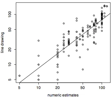
Figure 7.2. Cross-modal validation of adjective phrase acceptability judgments. log(lines) = -0.0335 + 0.96*log(numbers), R2 = 0.744.
As you can see in figure 7.2, looking at all of the raw data points in the data set, participants’ judgments of phrase acceptability using line length were correlated with their numerical estimates. The slope of this relationship is nearly exactly 1, but there is a certain amount of spread which seems to indicate that their impressions of the acceptability of the phrases were not as stable as were their impressions of line length.
“favorite” numbers given in the numerical estimates. For instance, the cluster of dots over x=2 indicates that the numerical estimate 100 (102) was given by many of the participants.
---R-note. I saved the raw line length and numeric estimate data in a text file “magest2.txt”.
> mag <- read.delim("magest2.txt")
Figure 7.2 was made with the following commands.
> summary(lm(log(mag$lines)~log(mag$numbers)))
> plot(mag$numbers,mag$lines,log="xy",xlab="numeric estimates",ylab="line drawing")
> abline(lm(log(mag$lines)~log(mag$numbers)))
---Now, finally, we are ready to consider the linguistic question under discussion, namely whether acceptability is a function of the distance on the Hetzron (1978) template of preferred adjective order. We are concerned primarily with the consequences of putting the adjectives in the
“wrong” order, testing the hypothesis that violations of the order predicted by the template will be more unacceptable the further the adjectives are from each other in the template.
I coded Hetzron distance as 1 if the adjectives are in the order predicted by the template, and 1 + the number of template slots that separate the adjectives when they were not in the correct order. I did this on the average distances in the four groups of experimental stimuli, so for each
participant there were five categories of stimuli - correct, and then incorrect order with adjectives from group 1, 2, 3, or 4. There were 12 students in my class, who participated in this experiment (thanks guys!). Five of them were native speakers of English and 7 were nonnative speakers of English.
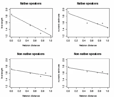
Figure 7.3. Adjective ordering acceptability (measured by line length responses (left column) or by numerical estimates of acceptability (right column), as a function of group number. Responses from native English speakers are in the top graphs and by nonnative speakers of English are in the bottom graphs.
Table 7.3 summarizes the line fits shown in figure 7.3. The linear fits (in this log-log
representation of the data) were generally quite good for both groups of participants, with three of the four R2 values near 0.9. The nonnative speakers produced functions that are about half as
than it was for the numerical estimation task. This may have been due to a tendency to limit the upper bound of their responses at 100.
Table 7.3. Analysis of an adjective ordering psychogrammatical law for native speakers of English, and nonnative speakers of English.
0.91 -0.19 numbers 0.75 -0.20 lines nonnative 0.89 -0.42 numbers 0.90 -0.61 lines native fit slope
In sum, this example magnitude estimation experiment illustrates the use of an empirical
technique to elicit acceptability judgments. The hypothesis I tested is a somewhat naive one, but I hope that this demonstration will be provocative enough to cause someone to want to use magnitude estimation to study syntax.
---R-note. Figure 7.3 was drawn with these R commands. I also used lm() to calculate the
regression coefficients used in the curve() commands here, and for the report of slopes and fits in table 7.3.
> nl <- c(70.5,33, 19, 26.3, 15.8) > fl <- c(52.6, 39.2, 31.8, 39.9, 31.5) > nn <- c(83.1, 38.8, 36.7, 38.1, 27.7) > fn <- c(59.9, 44.1, 40.8, 42.9, 37.4) > d <- c(1,3,5.5,7.33,10)
The Hetzron distance (d) that I entered into these graphs is one plus the number of slots that separate the adjectives in the template (see table 7.3) for those phrases in which the adjectives are in the wrong order. Phrases in which the adjectives were in the correct order were given a one on the distance axis (d) in these figures. The log10 of d then ranges from 0 to 1.
> par(mfrow(c(2,2))
> plot(log10(d),log10(nl),ylim = c(1.2,2),main="Native speakers", xlab="Hetzron distance", ylab="line length")
> curve(1.82853 - 0.60942*x,0,1,add=T)
,xlab="Hetzron distance", ylab="numeric estimate") > curve(1.88125 - 0.42488*x,0,1,add=T)
> plot(log10(d),log10(fl),ylim = c(1.2,2),main="Non-native speakers" ,xlab="Hetzron distance", ylab="line length")
> curve(1.70625 - 0.1996*x,0,1,add=T)
> plot(log10(d),log10(fn),ylim = c(1.2,2),main="Non-native speakers" ,xlab="Hetzron distance", ylab="numeric estimate")
> curve(1.76282 - 0.18694*x,0,1,add=T)
---7.3 Linear mixed effects in the syntactic expression of agents in English
In this section we will be using a data set drawn from the Wallstreet Journal text corpus that was used in the CoNLL-2005 (Conference on Computational Natural Language Learning) shared task to develop methods for automatically determining semantic roles in sentences of English.
Semantic roles such as agent, patient, instrument, etc. are important for syntactic and semantic descriptions of sentences, and automatic semantic role determination also has a practical
application, because in order for a natural language processing system to correctly function (say to automatically summarize a text) it must be able to get the gist of each sentence and how they interact with each other in a discourse. This kind of task crucially requires knowledge of semantic roles - who said what, or who did what to whom.
Well, that’s what the CoNLL-2005 shared task was. In this section, I’m just using their database for an example of mixed effects modeling asking a very simple (if not simplistic) question. We want to know whether the size (in number of words used to express it) of the noun phrase that corresponds to the “agent” role in a sentence is related to the size (again in number of words) of the material that comes before the clause that contains the agent expression. The idea is that expression of agent may be abbreviated in subordinate or subsequent clauses.
What we will do in this section is investigate a method for fitting linear “mixed effects” models where we have some fixed effects and some random effects. Particularly we will be looking at linear mixed effects models and a logistic regression extension of this approach to modeling linguistic data. As I mentioned in the introduction to the book, this is some of the most sophisticated modeling done in linguistic research and even more than with other methods
introduced in this book it is important to consult more detailed reference works as you work with these models. In particular, the book Mixed-effect Models in S and S-Plus by Pinheiro and Bates (2004) is very helpful.
to build linear mixed effects models that predict the size (in words) of the agent expression. Some examples will help to clarify how the data is coded. With “take” in the sense of “to acquire or come to have” (this is verb sense 01 for “take” in Verbnet), argument zero (A0) is the taker, and argument one (A1) is the thing taken. So the sentence “President Carlos Menem took office July 8” is tagged as:
(A0 President Carlos Menem) (V took) (A1 office) (AM July 8).
where the tag “AM” is a generic tag for modifiers. In almost all cases in the corpus A0 is used to tag the agent role.
In the longer sentence below, the clause containing “take” is embedded in a matrix clause “the ruling gives x”. The phrase “pipeline companies” is coded as A0, and “advantage” as A1. In addition to this, the fact that there was earlier material in the sentence is coded using the label N0. So the argument structure frame for the verb “take” in this sentence is:
(N0)(A0)(V=take)(A1)(A2)
According to industry lawyers, the ruling gives pipeline companies an important second chance to resolve remaining disputes and take advantage of the cost-sharing mechanism.
The question that we are concerned with in this example is whether there is any relationship between the number of words used to express the agent, A0, and the number of words earlier in the sentence, N0. There are a number of indeterminancies in the data that will add noise to our predictive models. The N0 labels do not contain information as to whether the target verb, “take” in the examples above, is the matrix verb of the sentence, or in an embedded clause. Additionally, the dependent measure that we are looking at here, the number of words used to express A0 is a very rough way of capturing the potential syntactic complexity of the agent expression (if indeed an agent is specifically mentioned at all). Nonetheless, this little exercise will help to demonstrate mixed-effects modeling.
7.3.1 Linear regression - overall, and separately by verbs
The relationship between the number of words used to express the agent (a0) and the number of words present in an earlier portion of the sentence (n0) is shown in figure 7.4. This figure
and experimenter error) are at work. We’ll be investigating our ability to detect patterns in such noisy data.
[image:16.612.95.501.255.626.2]The data in figure 7.4 are plotted on a log scale, and all of the analyses described here were done with log transformed data because the raw data are positively skewed (the size of a clause cannot be less than zero). The log transform removes some of the skewness and decreases the impact of some of the rare longer agent phrases (the longest of which was 53 words!).
The negative slope of the regression line in figure 7.4 (a simple linear regression predicting a0 from n0) indicates that, overall, there is a relationship between the size of the agent phrase (a0) and the size of the preceding words (n0). As the size of the preceding material increases the size of the agent clause decreases.
Although the linear regression model does find a significant relationship between a0 and n0 [t(30588)= -53.46, p<0.01] (see table 7.4), the amount of variance in a0 that is captured by this regression is only 8.5% (R2 = 0.085). The large number of observations in the corpus sort of
guarantees that we will find a “significant” effect, but the magnitude of the effect is small.
Table 7.4. Coefficients in an overall linear regression predicting a0 from n0.
Coefficients:
Estimate Std. Error t value Pr(>|t|) (Intercept) 1.146171 0.005827 196.68 <2e-16 *** vbarg$n0 -0.194533 0.003639 -53.46 <2e-16 ***
Additionally, the overall regression in figure 7.4 and table 7.4 assumes, incorrectly, that all of the verbs in the corpus have the same negative relationship between agent size and the size of the preceding material in the sentence. Furthermore, the overall regression assumes that each observation in the database is independent of all of the others, when we should suspect that observations from different verbs might systematically differ from each other. We have seen a situation like this in the chapter on psycholinguistics above (ch. 4) where we dealt with data containing repeated measurements over an experimental “unit” like people or language materials by performing separate ANOVAs for subjects as a random effect and items as a random effect. Mixed effects modeling (the topic of this section) is an alternative approach for handling data with mixed random and fixed factors, and is particularly appropriate for data with uneven numbers of observations on the random effects because it uses maximum likelihood estimation procedures (as is done in glm() for logistic regression) rather than least squares estimation. This is important for these agent complexity data because the number of observations per verb is not equal. “Say” occurs in the data set 8358 times while there are only 412 occurrences of “know”. (The implications of this asymmetry regarding the type of reporting in the Wall Street Journal is beyond the scope of this chapter.)
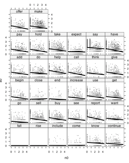
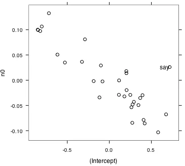
Figure 7.5 shows the intercept and slope values (with their confidence intervals) for 32 separate linear regressions - one for each of the verbs in the “vbarg” dataset. This figure shows that the intercept values particularly, and perhaps also the slope values, are different for different verbs. Two of the verbs (“rise” and “fall”) never occur with an explicit agent in this corpus, so they always have a0 of zero, while “say” tends to have a long a0 (an average length of about 5 words).
Because the verbs differ from each other in how n0 and a0 are related to each other, we need to devise a model that takes verb differences into account in order to correctly evaluate any general (verb independent) relationship between n0 and a0.
---R note. The agent complexity data are in the text data file “vbarg.txt”. This file has columns indicating the location of the verb in the sentence (vnum) counting from 0 up, the identity of the verb, the verb sense number (see http://verbs.colorado.edu/framesets/ for a complete listing), a text field that shows the argument structure of the verb, a number indicating the location of A0 in the argument structure where -1 means that A0 immediately precedes the verb and 1 means that A0 is immediately after the verb. The next column in the dataset similarly codes the location of the patient (A1). The remaining columns have numbers indicating the number of words that are used to express A0-A3 and that occur before (N0) or after (N1) the verb clause.
vnum,verb,sense,args,A0loc,A1loc,A0size,A1size,A2size,A3size,N0size,N1size 1,take,01,(N0)(A0)(V)(A1)(AM)(N1),-1,1,2,2,0,0,17,25
0,say,01,(A0)(V)(A1),-1,1,4,14,0,0,0,0
1,expect,01,(N0)(A0)(V)(A1),-1,1,1,12,0,0,5,0 0,sell,01,(A0)(AM)(V)(A1)(AM),-2,1,4,2,0,0,0,0 0,say,01,(A0)(V)(A1),-1,1,9,18,0,0,0,0
0,increase,01,(A0)(V)(A1)(A4)(A3),-1,1,3,2,0,5,0,0
The dataset can be read into R using read.delim() and you can see the column headings with names(), and an overall summary of the data with summary().
>vbarg <- read.csv("vbarg.txt") >names(vbarg)
[1] "vnum" "verb" "sense" "args" "A0loc" "A1loc" "A0size" [8] "A1size" "A2size" "A3size" "N0size" "N1size"
(-1 and 1) are as we would expect given the most frequent argument structures. A0size tends to be smaller than A1size and N0size.
I added log transformed counts for A0size and N0size with the following commands. These commands add new columns to the data frame.
> vbarg$a0 <- log(vbarg$A0size+1) > vbarg$n0 <- log(vbarg$N0size+1)
For some of the plotting commands in the nlme library it is very convenient to convert the data frame into a grouped data object. This type of data object is exactly like the original data frame but with a header containing useful information about how to plot the data; including a formula that indicates the response and covariate variables and the grouping variable, and some labels to use on plots.
> library(nlme) # this line loads the nonlinear mixed effects library > vbarg.gd <- groupedData(a0~n0|verb,vbarg)
The overall linear regression shown in figure 7.4 was done with the familiar lm() command and a simple plot() and abline() command. Note the use of the jitter() function to displace the points slightly during drawing.
> summary(lm(vbarg$a0~vbarg$n0)->alla0n0)
> plot(jitter(vbarg$a0,4)~jitter(vbarg$n0,4), ylab="Agent size (a0)", xlab="Preceding words (n0)")
> abline(lm(vbarg$a0~vbarg$n0))
The graph of 32 separate linear regression fits (figure 7.5) was produced using the very
convenient function lmList() in the nlme library of R routines. The formula statement for this command is the same as the one we use in a standard linear regression, except that after a vertical bar, a grouping factor is listed, so that in this lmList() statement, the data are first sorted
according to the verb and then the a0~n0 regression fit is calculated for each verb. The intervals() command returns the estimated regression coefficients for each verb, and gives the high and low bounds of a 95% confidence interval around the estimate.
> library(lattice) # graphics routines
> trellis.device(color=F) # set the graphics device to black and white > a0n0.lis <- lmList(a0~n0|verb,data=vbarg.gd)
> plot(intervals(a0n0.lis)) # figure 7.5
7.3.2 Fitting a linear mixed effects model - fixed and random effects
Linear mixed effects modeling uses restricted maximum likelihood estimation (REML) to fit a mixed effects model to the data. The model is specified in two parts. The first defines the fixed effects, which for this model is the formula a0~n0 to specify that we are trying to predict the (log) size of agent expression from the (log) size of whatever occurred prior to the verb clause. In the first model, the one I named “a0n0.lme”, the random component is identified as the grouping factor “verb” alone (random = ~ 1 | verb). This produces a separate intercept value for each verb, so that this model, unlike the overall regression, does not assume that average agent size is the same for each verb. We also do not let the most frequent verb dominate the estimate of the fixed effect. The difference between “say” and other verbs is captured in the random effects estimates, so that the fixed effects estimates represent the pattern of a0~n0 found across verbs - controlling for verb-specific differences.
The summary() results of this analysis suggest that there is a strong effect of n0 on a0 even after we control for the the different average size of a0 for different verbs (this is an interceponly model in which we assume that the slope of the n0 effect is the same for each verb). A t-test of the n0 coefficient shows that this fixed coefficient (-0.10) is reliably different from zero [t(30557)= -31.4, p<0.01].
Interestingly, it is not clear from the statistics literature how to compare the goodness of fit of a linear mixed effects model and a simple linear model. Because of the extra parameters involved in calculating the mixed effects model we should always have a better fit in absolute terms, and because the assumptions of the mixed effects model are a better match to the data than are the assumptions of the simple linear model, we should go ahead and use linear mixed effects. Then to compare different mixed effects models one uses a log likelihood ratio test that we will outline below.
I offer here two ways to compare the goodness of fit of linear mixed effects models and simple linear models. In one measure we take the root mean square of the residual errors as a measure of the degree to which the model fails to predict the data. These values are calculated using the R function resid(). An alternative measure suggested by Jose Pinhiero is to estimate the variance accounted for by each model (the R2). This method uses the functions fitted() and getResponse()
I would mention also that I used a cross-validation technique to measure the robustness of these models. In order to be sure that the model parameters were not overfitted to the data I calculated each model 100 times using 85% of the data set to calculate the model and then using the
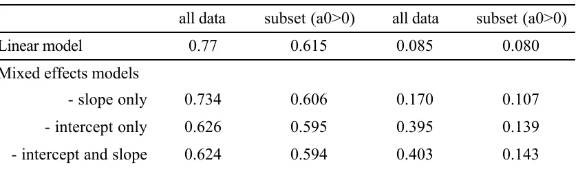
remaining 15% of the cases as a test set to evaluate the fit of the model. The RMS and R2 values that are shown in table 7.5 are the mean values found in the cross-validation runs. The standard deviation of the 100 RMS estimates was always at about 0.007. Thus, the 95% confidence interval for the RMS in the slope-only model for “all data” was 0.72-0.748. The standard deviation of the R2 was also extremely low at about 0.01. So, for example, the 95% confidence interval around the intercept-only “all data” model was 0.376-0.414. This encompasses the intercept and slope model, so we would conclude that adding slope coefficients to the model doesn’t significantly improve the fit of the model. Cross-validation is an extremely powerful way to determine the success of a statistical model. Without it we don’t really know whether a model will have acceptable performance on new data.
[image:22.612.75.495.421.557.2]Table 7.5 also shows that in exploring these data I also looked at five other mixed effects models. We turn now to these.
Table 7.5. Degree of fit measured two ways for various models of the verb argument size data.
Estimated R^2 RMS of the residuals
all data 0.403 0.143 0.139 0.395 0.107 0.170 0.080 all data 0.085 0.594 0.595 0.606 0.615 subset (a0>0) 0.624 - intercept and slope
0.626 - intercept only
0.734 - slope only
Mixed effects models
0.77 Linear model
subset (a0>0)
> a0n0.lme <- lme(a0~n0,data=vbarg.gd,random = ~ 1|verb) > a0n0.lme2 <- update(a0n0.lme, random = ~ n0|verb)
The random statement to get by-verb estimates of slope with no random intercept values is:
> a0n0.lme5 <- update(a0n0.lme, random = ~ n0 - 1|verb)
The RMS of the residuals is calculated from the output of resid(). The lme object has multiple levels of residuals depending on the number of grouping variables. Level one indicates that we want residuals taken using both fixed and random effects in the model. Level zero would give residuals from the fixed-effects only model.
> sqrt(mean(resid(a0n0.lme2,level=1)^2)) > sqrt(mean(resid(a0n0.lm)^2))
Estimated R2 values for lme() models can be obtained from the fitted values and the input values.
That is, the output of getResponse is a vector of the same values that you will find in vbarg$a0. So this statement simply takes the (square of the) correlation between the model’s predicted values for each verb in the data set, and the actual values in the data set. I have seen some complaints in on-line discussion groups that this estimate is incorrect, but it looks reasonable to me.
> cor(fitted(a0n0.lme2),getResponse(a0n0.lme2))^2
The cross-validation technique can be implemented with a small “for” loop which repeats the linear mixed effect model fitting operation one hundred times. I used two arrays to store the RMS and R2 results of each analysis. One trick in this procedure is that the split() command creates a new dataset, here called “xx” which has a TRUE subset which is about 85% of the observations, and a FALSE subset which is about 15% of the observations. Thus the designation “xx$`TRUE” is a dataset composed of 85% of the observations in “vbarg.gd”. The predict() command takes the model specification in mod and applies it to the dataset in xx$`FALSE` giving a set of predicted a0 argument sizes. We can then compare these predicted values with the actual values in the test set to derived RMS error or R2 “variance accounted for” measures of how well a model calculated from the training data fits the test set of data.
# here is a loop to split the vbarg data set - 85% training, 15% test # fit a nlme model to the training data,
# see how well the model predicts the argument size in the # test data, and collect the results for averaging/plotting
for (i in 1:100) {
# step 1: Split the data into training and test sets split(vbarg.gd,factor(runif(30590)>0.15))->xx
# step 2: estimate model parameters with the training set mod <-lme(a0 ~ n0, data=xx$`TRUE`,random = ~ 1|verb)
# step 3: get model predictions for the test set predict(mod,xx$`FALSE`)->pred
# calculate the root mean square error of the prediction RMS[i] <- sqrt(mean((pred-xx$`FALSE`$a0)^2))
Rsquared[i] <- cor(pred,xx$`FALSE`$a0)^2
}
mean(RMS) sd(RMS)
mean(Rsquared) sd(Rsquared)
---7.3.3. Fitting five more mixed effects models - finding the best model
We noticed in figure 7.5 that the intercept values for verb-specific linear regressions were
noticeably different, so we used a mixed effects model that has random effects for the intercepts. It is also apparent in figure 7.5, though, that the slope values relating n0 to a0 are also somewhat different from one verb to the next. Because we are especially interested in testing for a general trend for the slope across verbs it is important to control for verb-specific slope values. This is done by changing the specification of the random component of our model so that it includes an indication that we want to treat slope as a verb-specific random component (random = ~
n0|verb).
Now we can perform a couple of tests to determine (a) whether this new ‘verb-specific”
intercept and slope model is an improvement over the intercept only model and (b) whether there is still a fixed effect for slope.
The first of these is a test of whether a model with random effects for slope and intercept (verb-specific estimates) fits the data better than a model with only verb-(verb-specific intercept estimates. And this is done with a likelihood ratio test. The likelihood ratio is familiar from the discussion in chapter 5, Sociolinguistics, where we saw that the likelihood ratio is asymptotically distributed as X2, and we used this likelihood ratio test to compare models. The same procedure is used
“intercept and slope” model is 320, which is significantly greater than chance (p<0.001). This indicates that adding a random factor for slope significantly improved the fit of the model.
The second test we perform is a test of the fixed effects coefficients. After adding a random effect for slope, it may now be that any effect of n0 is to be found in the random slope values for the verbs, and there is then no remaining overall fixed effect for n0 on a0. A t-test, produced by the R summary() function, evaluating whether the n0 slope coefficient is significantly different from zero suggests that it is [t(30557)= -8.32, p < 0.001]. As in the simple linear regression, the slope coefficient is negative, suggesting that as the preceding material increases in size the agent phrase decreases in size.
---R note. The anova() function is defined to calculate the likelihood ratio test for comparing two mixed effects models (if they have different degrees of freedom).
> anova(a0n0.lme,a0n0.lme2) # intercept only vs. intercept and slope
Model df AIC BIC logLik Test L.Ratio p-value a0n0.lme 1 4 58410.54 58443.86 -29201.27 a0n0.lme2 2 6 58094.34 58144.31 -29041.17 1 vs 2 320.2043 <.0001
To see at-test of the fixed effects coefficients use the summary() function. This printout also suggests that the random effects for intercept and slope are negatively correlated with each other (Corr = -0.837) as shown in figure 7.7.
> summary(a0n0.lme2)
Linear mixed-effects model fit by REML Data: vbarg
AIC BIC logLik 58094.34 58144.31 -29041.17
Random effects: Formula: ~n0 | verb
Structure: General positive-definite, Log-Cholesky parametrization StdDev Corr
(Intercept) 0.46999336 (Intr) n0 0.06576902 -0.837 Residual 0.62275052
Fixed effects: a0 ~ n0
(Intr) n0 -0.814
Standardized Within-Group Residuals:
Min Q1 Med Q3 Max -2.5221371 -0.6895952 -0.1013437 0.4215483 5.0763747
Number of Observations: 30590 Number of Groups: 32
---This is visualized in figure 7.6. In this figure, the regression lines are those predicted by the linear mixed effects model with random verb effects for both the intercept and slope of the regression. Note that the slopes are negative for most verbs. It is also apparent that these data are not especially well fit by a linear function (at least one with only a single predictor variable), but the modeling results do suggest that amongst all this noise there is a relationship between a0 and n0 - we do seem to have identified n0 as a general predictor of agent size independent of any verb-specific effects.
agent phrase (a0) as a function of the (log) size of the phrase that occurs before the agent phrase (n0). Each panel in this plot corresponds to a verb-specific plot of the data shown in figure 7.4. This plot was generated with the R command: plot(augPred(a0n0.lme2), col=1, cex=0.2, lwd=2).
Figure 7.7. The estimates of the random effects in the mixed effects model of the verb argument data. Each dot shows the intercept and slope parameters for one of the verbs (“say” is the only one labeled). The command to produce this graph was: pairs(a0n0.lme2,~ranef(.),id=~verb=="say",adj=1.3)
If we hypothesize that agentless (a0=0) clauses are more likely in embedded clauses (at least some of the sentences with n0>0) as the scatter plots in figure 7.6 might suggest, then it may be that the number of agentless sentences in which a verb appears determines both the slope and the intercept of the a0~n0 regression. I tested whether the presence of agentless clauses might be the source of the finding that size of agent phrase is predicted by size of prior material by rerunning the analyses with a subset of the vbarg.txt dataset from which I removed agentless sentences.
The conclusion we draw from this analysis of cases in which there was an overt agent expression is no different from the conclusion we arrived at using the whole data set. Even allowing for random verb-specific effects for both the average size of the agent phrase (the intercept) and the relationship between agent phrase size and size of prior material (the slope), there was a
significant overall fixed effect of N0size on agent phrase size [coef = -0.108, t(21822) = -16, p < 0.001]. Recall that the slope coefficient from the bestfitting model of the whole data set was -0.101, almost the same as the slope value found in this analysis of a subset of data. The best fitting lines of the two analyses are plotted against the whole dataset in figure 7.8.
---R note. I used the subset() function to remove agentless clauses and then used lme() and update() to fit the mixed effects model to the subset.
> vbarg.subset <- subset(vbarg,a0>0) # extract the subset > vbarg.subset.gd <- groupedData(a0~n0|verb,vbarg.subset)
> a0n0.lme4 <- lme(a0~n0, data=vbarg.subset.gd, random = ~ 1|verb)
> a0n0.lme5 <- update(a0n0.lme4, random = ~ n0 - 1|verb) # model fitting > a0n0.lme3 <- update(a0n0.lme4, random = ~ n0|verb)
> anova(a0n0.lme4,a0n0.lme3) # intercept only vs. intercept and slope
Model df AIC BIC logLik Test L.Ratio p-value a0n0.lme4 1 4 39450.03 39481.99 -19721.01 a0n0.lme3 2 6 39412.69 39460.64 -19700.35 1 vs 2 41.33428 <.0001
> anova(a0n0.lme5,a0n0.lme3) # slope only vs. intercept and slope
Model df AIC BIC logLik Test L.Ratio p-value a0n0.lme5 1 4 40246.02 40277.99 -20119.01 a0n0.lme3 2 6 39412.69 39460.64 -19700.35 1 vs 2 837.3299 <.0001
I would note here that the lme object can be passed to anova() for a test of fixed effect factors in a mixed effects model. In these models I didn’t use this because n0 is a numeric variable and hence only a single coefficient is estimated. In this case the t-value returned by summary() suffices - and is the square-root of the F-value reported by anova(). But if you have a multilevel factor there will be a t-value for each dummy variable coefficient used to represent the levels of the factor, and thus anova() is a handy way to test for an overall effect of the factor.
> anova(a0n0.lme3)
numDF denDF F-value p-value (Intercept) 1 21822 1823.516 <.0001 n0 1 21822 256.255 <.0001
---7.4 Predicting the dative alternation - logistic modeling of syntactic corpora data
Bresnan, Cueni, Nikitina, and Baayen (2005) published an elegant paper describing a series of logistic regression analyses of the English dative alternation. They were also kind enough to share their data with me, so this section describes how they analyzed their data. I also agree with the larger point of their paper and so I’ll mention here that this analysis of the syntactic
realization of data is an important demonstration of the gradient, non modular nature of linguistic knowledge. All-or-none, deterministic rules of grammar are an inadequate formalism for capturing the richness of linguistic knowledge. This basic outlook is one of the main reasons that I wrote this book (here finally in the last section of the last chapter of the book I reveal my motives!). I think that for linguistics as a discipline to make any significant strides forward in our
understanding of language, linguists need to be equipped with the tools of quantitative analysis.
So, let’s see what the dative alternation situation is about and how Bresnan et al. used statistical analysis of corpus data to understand the facts of dative alternation.
Of the two alternative ways to say the same thing:
(1a) That movie gave the creeps to me. (1b) That movie gave me the creeps.
The first is probably not as acceptable to you as the second. The question addressed by Bresnan et al. is to account for this preference. Sentences (1a) and (1b) illustrate the dative alternation in which the recipient (“me” in these sentences) can be expressed in a prepositional phrase “to me” or as a bare noun phrase. So sentence (1a) illustrates the prepositional dative structure and sentence (1b) illustrates the double object dative structure.
Although the prepositional structure (1a) is dispreferred, it doesn’t take much investigation to find sentences where the prepositional dative structure is probably better. Consider for example sentences (2a) and (2b):
(2a) I pushed the box to John. (2b) I pushed John the box.
Here it is likely that you will find (2a), the prepositional structure, to be preferable to (2b).
than (3b).
(3a) This will give the creeps to just about anyone. (3b) This will give just about anyone the creeps.
Whether or not the theme has been mentioned more recently in the discourse (has greater discourse accessibility) affects realization of the dative - such that the given (discourse accessible) argument is more likely to occur just after the verb. For example, sentence (2a) is more likely in discourse fragment (4a) in which “box” is given in prior discourse context, while sentence (2b) is more likely in a discourse context in which John is given (4b).
(4a) I got down a box of crayons. I pushed the box to John.
(4b) John is one of those people who has to see for himself. I pushed John the box.
This factor in dative alternation reflects an interesting constellation of factors that seem to influence the order of verb arguments conspiring (in English at least) to “save the good stuff 'til last”.
- given information precedes new - pronouns precede nonpronouns - definites precede nondefinites - shorter NPs precede longer NPs
These factors can be evaluated in dative alternation.
---R note. You will find the Bresnan et al. (2005) dative data in the file “BresDative.txt”. This is a recoding of their original data file in which I used mnemonic labels for the codes that they applied to each example. You will note that the results discussed in this chapter are slightly different from the results given in Bresnan et al. This is because a couple of minor predictive factors that they used in their models are not available in this data set.
> dat <- read.table("BresDative.txt",header=T) > names(dat)
[1] "real" "verb" "class" "vsense" "animrec" "animth" [7] "defrec" "defth" "prorec" "proth" "accrec" "accth" [13] "ldiff" "mod"
> attach(dat) > table(mod)
mod
switchboard wallstreet 2360 905
We will use the Switchboard and Wall Street Journal subsets separately so we’ll pull these data into separate data frames.
> subset(dat,mod=="switchboard") -> SwitchDat > subset(dat,mod=="wallstreet") -> WSJDat
---Bresnan et al. (2005) coded 3265 datives taken from two corpora of American English. The coding scheme marked the realization of the dative (PP = Prepositional construction, NP = double object construction) and then for each instance marked the discourse accessibility, definiteness, animacy, and pronominality of the recipient and theme. They also noted the semantic class of the verb (abstract, transfer, future transfer, prevention of possession, and communication). Finally, we also have in the data set a measure of the difference between the (log) length of the recipient and (log) length of the theme.
Obviously, the collection of such a carefully coded dataset is nine-tenths of the research. The statistical analysis is the easy part (especially with a helpful chapter like this!), and no statistical analysis in the world can compensate for an unrepresentative, incomplete, or too small dataset. Many thanks to Joan Bresnan and colleagues for so cheerfully sharing this exemplary dataset with me.
7.4.1 Logistic model of dative alternation
The variable that we wish to predict, or wish our model to account for, is the realization of the dative. This is a binary outcome variable - the person either used a preposition construction or a double object construction. In other words, the analysis problem here is exactly what we saw in the sociolinguistics chapter with variable pronunciation outcomes.
So it should come as no surprise that we can use the generalized linear model [glm()] to fit a logistic regression predicting dative outcome from discourse accessibility, semantic class, etc.
> modelA <-glm(real ~ class + accrec + accth + prorec + proth + defrec + defth + animrec + ldiff, family=binomial, data=SwitchDat)
> summary(modelA)
Call:
glm(formula = real ~ class + accrec + accth + prorec + proth + defrec + defth + animrec + ldiff, family = binomial)
Deviance Residuals:
Min 1Q Median 3Q Max -2.60321 -0.30798 -0.15854 -0.03099 3.33739
Coefficients:
Estimate Std. Error z value Pr(>|z|) (Intercept) 0.3498 0.3554 0.984 0.32503 classc -1.3516 0.3141 -4.303 1.68e-05 *** classf 0.5138 0.4922 1.044 0.29651 classp -3.4277 1.2504 -2.741 0.00612 ** classt 1.1571 0.2055 5.631 1.80e-08 *** accrecnotgiven 1.1282 0.2681 4.208 2.57e-05 *** accthnotgiven -1.2576 0.2653 -4.740 2.13e-06 *** prorecpronom -1.4661 0.2509 -5.843 5.13e-09 *** prothpronom 1.5993 0.2403 6.654 2.85e-11 *** defrecindef 0.8446 0.2577 3.277 0.00105 ** defthindef -1.1950 0.2202 -5.426 5.78e-08 *** animrecinanim 2.6761 0.3013 8.881 < 2e-16 *** ldiff -0.9302 0.1115 -8.342 < 2e-16 ***
---Signif. codes: 0 ‘***’ 0.001 ‘**’ 0.01 ‘*’ 0.05 ‘.’ 0.1 ‘ ’ 1
(Dispersion parameter for binomial family taken to be 1)
Null deviance: 2440.1 on 2359 degrees of freedom Residual deviance: 1056.9 on 2347 degrees of freedom AIC: 1082.9
Number of Fisher Scoring iterations: 8
---Let’s see how to interpret this model by discussing a few of the coefficients. These are listed under “Estimate” in the summary() of the model.
was used only 12% of the time, while when the recipient was not given the prepositional dative construction was used 58% of the time. The regression coefficient was 1.13 indicating a positive correlation between “not given” and “PP” - prepositional dative construction. One way to interpret the logistic regression coefficient is in terms of the odds ratio. In this case, the
Table 7.6. The coefficients and observed percentages of prepositional realizations of dative (%PP) are shown for several of the factors in a logistic model of dative realization in the Switchboard corpus.
Percent Prepositional Dative (PP) 49% 19% 11% 44% 64% 17% 13% 62% 60% 12% 62 % Not Animate Animate Animacy of Recipient (2.68)
Not Definite Definite Definiteness of Theme (-1.2)
Not Definite Definite Definiteness of Recipient (0.85)
Not Pronoun Pronoun Pronominality of Theme (1.6)
Not Pronoun Pronoun Pronominality of Recipient (-1.47)
12% Not Given
Given Accessibility of Theme (-1.26)
58% Not Given
12% Given
Accessibility of Recipient (1.13)
All of the other factors in the logistic regression model of dative alternation fit the general idea that “good stuff” (new, non-pronominal, definite, animate objects) comes later in the sentence.
7.4.2 Evaluating the fit of the model
So far here is what we have. Using logistic regression we have found that several factors are included in a predictive statistical model of dative realization, and these factors are consistent with a harmonic set of constraints on syntactic forms.
It is reasonable to ask at this point whether this statistical model is really very good at predicting the realization of dative in English, because it could be that our model does account for some nonrandom component of variance in the corpus data, but fails to correctly predict the majority of cases. This can happen when we fail to include some important factor(s) in the model. In this section we will look at three ways to evaluate the fit of the logistic model.
The first is to consider how well the model predicts the training data. The general linear model fitting procedure glm() finds model parameters (the regression coefficients) that produce the best possible predictions given the predictive factors included in the model. Therefore, our first test is to evaluate the goodness of this fit. The function predict(modelA) returns a “prediction score” for each data case in the data frame used to find the coefficients in modelA. This is the
Figure 7.9 Prediction scores for the Switchboard dative data.
To evaluate the statistical model we tabulate the predicted and actual realizations it produces using these prediction scores. The result is that for 91% of the data cases the model gives the correct prediction. Tabulating comparisons of model predictions and actual realizations for various subsets of data will show where this model may be more or less accurate. Note that the imbalance of realization in the data set makes it possible to produce a model with no parameters at all that correctly predicts 79% of the data cases by simply predicting that dative is always realized in the double object construction (because 79% of the cases are actually realized as double objects). This is the lower bound of possible model predictions. Still, 91% correct predictions from a model that only uses a few general properties of sentences is pretty good.
scores for the test sentences. This split-glm-predict procedure is repeated 100 times to get a stable estimate of how well the statistical model can predict dative realization in sentences that were not part of the training data.
Testing a model on unseen data is an important test of a model because it is possible to “over-fit” a statistical model and have model parameters that capture information in only one or two outlier observations rather than capturing generalizations over many observations. Testing on never-before-seen data is a good way to test for over-fitting.
The dative alternation model gets an average of 91% correct in one hundred random splits into 85% training and 15% test data. This is very close to the 91% correct observed for the model fit to all of the data and the good match between the two procedures indicates that the model is not over fit. The distribution of these 100 test results is shown in figure 7.10.
Finally, we can evaluate the validity of the statistical model of dative alternation by testing its predictions on a completely different data set. Recall that in addition to Switchboard, Bresnan et al. coded 905 datives from the Wall Street Journal corpus. Switchboard is a conversational speech corpus in which about 79% of datives are realized in the double object construction, while the Wall Street Journal corpus, as the name implies, is corpus of written and edited text. The dative is usually also realized in the double object construction in this corpus, but at 62% the base probability of double object is quite a bit lower. If the model is capturing something real about English syntax then we would expect good predictive power despite these corpus differences.
Using the predict() function to calculate dative scores for the Wall Street Journal corpus we find a much higher number of predicted PP cases than in Switchboard, and also good prediction
Figure 7.10. Distribution of 100 tests of the logistic model of dative alternation showing that most of the 100 random splits (into training and testing data sets) produced correct prediction of the dative alternation in over 90% of the test sentences.
---R-note. The commands for our three ways of evaluating the dative alternation logistic regression are shown in this note.
The first method, using predict, is a vision of simplicity. Simply compare the prediction score with the actual realization code.
>table((predict(modelA)>0.0)==(SwitchDat$real=="PP"))
> 2159/(2159+201)
[1] 0.9148305
To get a little more information about the fit we can cross-tabulate the prediction score accuracy as a function of the predictor variables. For example, discourse accessibility of the recipient was a less consistently useful predictor than was the accessibility of the theme:
> table((predict(modelA)>0.0)==(SwitchDat$real=="PP"),accrec)
accrec
given notgiven FALSE 98 103 TRUE 1773 386 % correct 95% 79%
> table((predict(modelA)>0.0)==(SwitchDat$real=="PP"),accth)
accth
given notgiven FALSE 40 161 TRUE 401 1758 % correct 91% 92%
Bresnan et al. also showed a useful cross-tabulation (their table 1) produced with this command:
> table((SwitchDat$real=="PP"),predict(modelA)>0.0)
NP PP NP 1788 71 96% PP 130 371 74%
The following commands produce figure 7.9.
> hist(subset(predict(modelA),real=="NP"), dens=c(10), angle=c(45), main="",xlab="prediction score",xlim=c(-10,10))
> hist(subset(predict(modelA),real=="PP"), add=T,breaks=c(-9,-8,-7,-6,-5,-4,-3,-2,-1,0,1,2,3,4,5,6,7,8,9,10),col="gray")
> legend(5,350,legend=c("NP","PP"),fill=c("black","gray"),density=c(10,-1), angle=c(45,-1),cex=1.5)
The second evaluation method discussed in this section involves the use of a “for” loop to
false coding whether the random number was above or below 0.15. This produces a split that has approximately 15% of the data cases in the “TRUE” subset and 85% in the FALSE subset.
> split(SwitchDat,factor(runif(2360)>0.15))->xx # split approximately 85/15
> table(xx$`TRUE`$real) # this set will be used for training a model
NP PP 1571 441
> table(xx$`FALSE`$real) # this set will be used for testing the model
NP PP 288 60
# here is a loop to split switchboard - 85% training, 15% test # fit a glm model to the training data,
# see how well the model predicts the Dative realization in the # test data, and collect the results for averaging/plotting
pcorrect<-array(dim=100) # allocate space for results for (i in 1:100) {
# step 1: Split the data into training and test sets split(SwitchDat,factor(runif(2360)>0.15))->xx
# step 2: estimate model parameters with the training set
mod <-glm(real ~ class + accrec + accth + prorec + proth + defrec + defth + animrec + ldiff, family=binomial, data=xx$`TRUE`)
# step 3: get model predictions for the test set predict(mod,xx$`FALSE`)->pred
# bookkeeping 1: tabulate the responses and correct and incorrect table((pred>0.0)==(xx$`FALSE`$real=="PP"))->tab
# bookkeeping 2: save the probability of a correct answer pcorrect[i] <- tab[2]/(tab[1]+tab[2])
}
> mean(pcorrect)
[1] 0.9107247
> hist(pcorrect) # this produces figure 7.10
Here is how to use the model built on the Switchboard corpus to predict dative realization in the Wall Street Journal corpus. We get 83% correct on the WSJ.
> predict(modelA, WSJDat)
> table((WSJDat$real=="PP")==(predict(modelA,WSJDat)>0.0))
FALSE TRUE
151 754 83% correct
> table((WSJDat$real=="PP"),predict(modelA,WSJDat)>0.0)
NP PP
NP 510 47 92% PP 104 244 70%
---7.4.3 Adding a random factor - mixed effects logistic regression
So far we have pooled sentences regardless of the verb used in the sentence, as if which particular verb is used doesn’t matter. This is an erroneous assumption. For whatever reason, the
particular semantics of the verb, some fossilized conventions associated with a particular verb, or whatever, it is apparent that some verbs are biased toward the double object construction while others are biased toward the prepositional dative. More than this it seems clear that verb bias relates to the particular sense of the verb. For example, “pay” in its transfer sense (e.g. “to pay him some money”) tends to take an animate recipient and tends to appear in the double object construction, while “pay” in a more abstract sense (e.g. “to pay attention to the clock”) tends to take an inanimate recipient and tends to appear in the prepositional dative construction. We don’t know which is the true predictive factor - the particular verb sense, or general predictive factors such as the animacy of the recipient, or some combination of these random (verb) and fixed (animacy) factors.
choice (double object versus prepositional dative) and thus we need to fit a mixed effects logistic regression model. The R function glmmPQL() - generalized linear mixed models fit using
Penalized Quasi-Likelihood - is analogous to lme() in that we specify a fixed component and a random component of the model, while also providing the capability of glm() to allow us to fit a logistic model.
In the case of dative alternation we specify the fixed factors in our model exactly as we did with the glm() function, but we also add a random formula (random= ~1/vsense) which adds an intercept value for each verb sense (where the verb senses are pay.t for “pay” in the transfer sense, pay.a for “pay” in the abstract sense, etc.) to account for bias attributable to each verb sense. The main question we have is the same type of question we have in repeated measures analysis of variance - if we include a term to explicitly model particular verb sense biases do we still see any effect of discourse accessibility, pronominality, definiteness, animacy, or argument size difference? If these factors remain significant even when we add a factor for verb sense then we have support for a model that uses them as general predictive factors.
Figure 7.11 A comparison of logistic regression coefficients for a glm() model with the fixed effects shown on the x axis of the figure, and a glmmPQL() mixed effects model with the same fixed effects but also treating verb sense as a random effect.
---R note. The mixed effects logistic model is fit with the function glmmPQL() which can be found in the MASS library of routines. So load MASS.
> library(MASS)
The model formula for glmmPQL() is just like the formulas that we have used before. Adding negative one to the list of factors removes the intercept so that we will then have coefficients for each semantic class. What is new in this model is that we can specify a random factor as with lme() in section 7.6. Here we specify that each verb sense is modeled with a different intercept value. We also specify the binomial link function which causes this to be a logistic regression model in the same way that family=binomial produces a fixed effects logistic regression model with glm().
> modelB <-glmmPQL(real ~ -1+
class+accrec+accth+prorec+proth+defrec+defth+animrec+ldiff, random = ~1|vsense, family=binomial, data=SwitchDat)
> summary(modelB)
Linear mixed-effects model fit by maximum likelihood Data: SwitchDat
AIC BIC logLik NA NA NA
Random effects:
Formula: ~1 | vsense
(Intercept) Residual StdDev: 2.214329 0.774242
Variance function:
Structure: fixed weights Formula: ~invwt
Fixed effects: real ~ -1 + class + accrec + accth + prorec + proth + defrec + defth + animrec + ldiff