Bayesian Sequential Track Formation

Bayesian sequential track formation

Ángel F. García-Fernández, Mark R. Morelande, Jesús Grajal

Abstract—This paper presents a theoretical framework for track building in multiple target scenarios from the Bayesian point of view. It is assumed that the number of targets is fixed and known. We propose two optimal methods for building tracks sequentially. The first one uses the labelling of the current multitarget state estimate that minimises the mean square la-belled optimal subpattern assignment error. This method requires knowledge of the posterior density of the vector-valued state. The second assigns the labelling that maximises the probability that the current multitarget state estimate is optimally linked with the available tracks at the previous time step. In this case, we only require knowledge of the random finite set posterior density without labels.

Index Terms—Target labelling, multiple target tracking, Bayesian framework, random finite sets

I. INTRODUCTION

Multitarget tracking systems should solve two basic prob-lems. The first one is to estimate the number of targets and their states at the current time. The second one is to connect target state estimates that belong to the same target along time to form tracks. Classic approaches to multitarget tracking that perform these aims are, for example, multiple hypothesis tracking (MHT) [1] and joint probabilistic data association (JPDA) [2]. The random finite set (RFS) framework is another approach to perform these tasks. However, most of the de-veloped algorithms within the RFS framework have focused on the first problem and do not deal with the second problem from a theoretically sound perspective, e.g., probability hypothesis density (PHD) filter, cardinalised PHD (CPHD) filter or the multitarget multi-Bernoulli (MeMBer) filter [3], [4].

In the Bayesian approach, all the information of interest about target states at all time steps is contained in its joint probability density function (PDF) given the measurements [5], which we refer to as the trajectory posterior PDF. This suggests that principled approaches to track building should be obtained from this PDF. Nevertheless, most approaches to multiple target tracking focus on filtering posterior density computation because of the difficulty of approximating the

Copyright (c) 2014 IEEE. Personal use of this material is permitted. However, permission to use this material for any other purposes must be obtained from the IEEE by sending a request to [email protected]. Ángel F. García-Fernández was with Departamento de Señales, Sistemas y Radiocomunicaciones, Universidad Politécnica de Madrid, Ciudad Universit-aria s/n, 28040 Madrid, Spain (email: [email protected]). Mark R. Morelande is with the Department of Electrical and Electronic Engineering, The University of Melbourne, Parkville, Victoria 3010, Australia (email: [email protected]).

Jesús Grajal is with Departamento de Señales, Sistemas y Radiocomunic-aciones, Universidad Politécnica de Madrid, Ciudad Universitaria s/n, 28040 Madrid, Spain. (email: [email protected]).

This work was supported in part by the Spanish national research and de-velopment program under Projects TEC2011-28683-C02-01 and Comonsens (Consolider-Ingenio 2010, CSD2008-00010).

trajectory posterior PDF. Therefore, the usual approach to track building, which will also be adopted here, is based on filtering posteriors.

the following paragraphs.

In the first algorithm to optimal track building, we minimise the mean square LOSPA (MSLOSPA) error. Therefore, in this approach, the objective is to choose the labelling of the estimate that is closest to the true multitarget state, according to LOSPA. For low penalty of labelling error in LOSPA, the MSLOSPA error can be decomposed into two terms, the MSOSPA error, which does not take labels into account, plus the mean labelling error cost (MLEC). Considering this decomposition, the labelling of the multitarget estimate that minimises the MSLOSPA error is the one that minimises the MLEC. The MLEC depends on the optimal labelling probabilities. These are simply calculated using probability theory and the definition of optimal labelling of a multitar-get state estimate. They also provide useful information, for instance, if it is necessary to distinguish between friendly and enemy vehicles that get in close proximity and then separate [15]. Although many papers use the concepts of labelling and labelling probabilities, these concepts have not been clearly defined in the literature yet. To the authors’ knowledge, the fact that the (optimal) labelling probabilities depend on an estimate and a metric was first indicated in [9, Sec. 5.3] for a two-target case. In general, this has been usually overlooked in the literature [15]–[18]. In [19], the labelling probabilities for a two-target case are those previously indicated in [9, Sec. 5.3]. In [20], the authors provide a definition of labelling probabilities. However, a proper definition of optimal target labelling probabilities should first define what optimal target labelling is and the probabilities should just be calculated using probability theory.

In some cases, we are interested in minimising track switch-ing rather than obtainswitch-ing the labellswitch-ing of the estimate that is closest to the true multitarget state, e.g, as in [13]. In this paper, we formulate this problem in a principled approach as the selection of the labelling of the estimate that maximises the probability that the current multitarget state is optimally linked with the tracks available at the previous time step. On the whole, this method of track building outperforms the one based on the MSLOSPA error. As opposed to the conventional approach, we show that this track building procedure does not require a labelled state, i.e., we can use an unlabelled set to represent the multitarget state. As we explain in the paper, this result is of great utility in the design of multitarget tracking algorithms.

The remainder of the paper is organised as follows. In Section II, we formulate the problem. The first procedure for track formation based on labelled states is explained in Section III. The second procedure for track building, which minimises track switching and does not require a labelled state, is explained in Section IV. Both approaches to track building are compared in Section V. A numerical example that illustrates the ideas put forward in this paper is given in Section VI. Finally, conclusions are drawn in Section VII.

II. PROBLEM FORMULATION

The multitarget state vector at time k is Xk ₌

h

xk₁T, xk₂T, ..., xkt

TiT

∈ Rtnx _{where x}k j ∈ R

nx _is

the state vector at time k for target j ∈ {1, ..., t}, t is the known target number and T denotes transpose. The mul-titarget state can be equivalently represented by a labelled

set

_h

xk 1

T

, l1

iT

,h xk 2

T

, l2

iT

, ...,h xk t

T

, lt

iT

where

lj ∈R represents the jth label. Labels are unique, assigned

deterministically and do not change with time. This implies that vector and labelled set notations are equivalent for fixed and known number of targets. The labels of the labelled set are implicit in the ordering inherent in the multitarget state vector components.

The multitarget state along time is modelled as a Markov process with a transition densityf ·Xk−1

. At time k, the multitarget state vector is observed through noisy measure-ments, which are usually represented as a vector zk _∈

Rnz,1

[6] or as a set Zk _⊂

Rnz,2 [3]. We use zk to denote the

measurements in the rest of the paper but our paper is general and we can use Zk _{instead. The likelihood of X}k _after observingzk _{is denoted by` z}k

Xk

.

In Bayesian filtering, all the information of interest about

Xk _{is included in the posterior PDFπ}k_{(·)of the state given} the sequence z1:k _{= z}1_,z2_{, ...,z}k

of measurements up to time k. Given a prior π0_{(·) at time 0, the transition density} and the likelihood at every time step, the posterior PDF can be calculated recursively in two stages: prediction and update [21].

This recursion is usually intractable so it must be approx-imated. For instance, particle filters (PFs) can be applied for any type of transition density and likelihood function as PFs are general Bayesian filtering algorithms. If there is a point detection measurement model, in which there is a collection of measurements and each measurement can be originated from clutter or a target [3], [5], more specific algorithms such as MHT or JPDA [2] can be used.

However, this paper does not deal with posterior PDF approximation but with how to extract target labelling in-formation and build tracks in a principled way regardless of measurement function or the approximation we perform. We therefore assume that the posteriorπk_{(·)is known although,} in practice, the track building procedures indicated in this paper can be carried out using an arbitrary posterior PDF approximation. In the rest of this section, we formulate the problem of track formation.

Track formation

Multitarget tracking systems should estimate target states and link target state estimates over time to form tracks. The first goal is attained by providing individual target state estim-ates, which can be represented by setsXˆk =ˆxk₁,ˆxk₂, ...,xˆk_t

Euclidean distance)1[11] or an approximation [15], [22], [23]. In this paper, we set aside this problem, which is already solved theoretically, and develop optimal approaches to link these optimal target state estimates to form tracks. In this context, track formation consists of selecting the labels, i.e., the order in the elements of Xˆk, to build the multitarget state estimateXˆk_{. The sequence of multitarget state estimates}

ˆ

Xk _{k = 0,1,2, ... forms the tracks as it provides the target} estimates that belong to the same target at different time steps. This paper is especially concerned with providing two methods for sequential track building. That is, we have the tracks up to a certain time k−1, which are given by Xˆl

l = 0,1,2, ..., k−1. When the measurement at time k is received, we assume we obtain Xˆk at time k. Sequential track building consists of labelling Xˆk without modifying the available tracks. This implies that track building is performed while filtering and we directly provide tracks as output.

III. TRACKS THAT MINIMISEMSLOSPAERROR

In this section we indicate how to build tracks by selecting the labelling of the multitarget state set estimate Xˆk _that minimises the MSLOSPA error under the approximation of low penalty of labelling error. Before explaining this in Section III-D, we first review the LOSPA metric in Section III-A, define the notion of optimal labelling in Section III-B and explain how to calculate the optimal labelling probabilities in Section III-C.

A. Labelled OSPA metric

In order to build tracks, we use the OSPA metric for labelled sets defined in [14]. We represent the permutations of vector [1, ..., t]T as vectors φ_i = [φi,1, ..., φi,t]

T

i ∈ {1, ..., t!}. Then, the LOSPA distance between multitarget vectors Ak = h ak1

T

, ak2

T

, ..., akt

TiT

∈ Rtnx _and

Bk₌h _bk

1

T

, bk 2

T

, ..., bk t

TiT

∈Rtnx is [24]

d Ak,Bk

=





1

t i∈{min1,...,t!} 



t

X

j=1

bpak_j,bk_φi,j+αpδ[j−φi,j]



 



1/p

(1)

where δ[·] is the complement of the Kronecker delta, i.e.,

δ[j] = 0ifj= 0andδ[j] = 1otherwise,α >0,1≤p <∞

and b(·,·) is a metric on the space Rnx_{. In [14] the authors} include another parameter p0, we set p0 =pfor simplicity.

1_{ThesquareOSPA metric (OSPA to the power of two) withp= 2,c=∞} and Euclidean distance is equivalent to the OSPA metric withp = 1,c= ∞and square Euclidean distance as base metric. Therefore,Xˆk_{is also the}

minimum mean OSPA estimator for the OSPA withp= 1,c=∞and square Euclidean distance. In this paper, we always refer to the casep= 2,c=∞

and Euclidean distance. Nevertheless, the whole paper can be rewritten using the OSPA withp= 1,c=∞and square Euclidean distance.

Table I: LOSPA betweenXˆk_andXk_{= [−10,0,10]}T

EstimateXˆk _{LOSPA(α= 0.1) LOSPA(α= 1)}

[−10.1,0.1,10.1]T _{0.1 0.1}

[0.1,−10.1,10.1]T p

0.12_{+ 0.02/3} p

0.12_{+ 2/3}

[10.1,−10.1,0.1]T p0.12_{+ 0.03/3} p

0.12_{+ 3/3}

Illustrative example: We illustrate how the LOSPA metric

works in a simple example. Let us assume there are three unidimensional targets and the multitarget state is Xk ₌ [−10,0,10]T. That is, target 1 is at -10, target 2 is at 0 and target 3 is at 10. We use the Euclidean metric forb(·,·)with

p= 2. The LOSPA distance betweenXkand several estimates ˆ

Xk, which only differ in their labelling, are given in Table I. As all the estimates only differ in their labelling, they have the same OSPA distance, which is 0.1. This implies that all the estimates have the same accuracy as regards where the targets are. However, the first estimate is closer in the LOSPA sense than the rest. The higher αis, the more the metric penalises wrong labelling/ordering.

B. Optimal labelling of a multitarget state estimate

In this section, we provide the definition of optimal la-belling of a multitarget state estimate. Then, we derive one of its properties and provide an illustrative example. Let

Γφ_i Xk =

xk φi,1

T

,xk φi,2

T

, ...,xk φi,t

TT

be the

permutation of Xk _{indicated by φ}

i over single target states, e.g., fort = 2, φ₁ = [1,2]T and φ₂ = [2,1]T, Γφ1 X

k

=

h xk

1

T

, xk 2

TiT

andΓφ₂ Xk=

h xk

2

T

, xk 1

TiT

.

Definition 1. The optimal labelling of a multitarget state

estimateXˆk ₌h _xˆk 1

T

, xˆk 2

T

, ..., xˆk t

TiT

at timek is the

vectorφ˜ =hφ˜1, ...,φ˜t

iT

such that

˜

φ=φi?: i?= arg min i∈{1,...,t!}

dXˆk,Γφ_i Xk

. (2)

As proved in Appendix A, the optimal labelling corresponds to the labels ofXˆk_{that minimise the LOSPA betweenX}k_and

ˆ

Xk_.

The following property is met for the optimal labelling of multitarget state estimates:

Lemma 2. The optimal labelling of the multitarget state

estimate does not depend on αand can be written as

˜

φ=φ_i?: i?= arg min i∈{1,...,t!}





1

t

t

X

j=1

bpˆxk_j,xk_φi,j 



1/p

.

Lemma 2 is proved in Appendix B and indicates that the optimal labelling is the order of the true multitarget state that determines the OSPA.

Table II: Optimal labelling of several multitarget state estimates for

Xk_{= [−10,0,10]}T

EstimateXˆk _{Optimal labellingφ}˜ _N˜ [−10.1,0.1,10.1]T _[1,2,3]T ₃

[0.1,−10.1,10.1]T _[2,1,3]T

1 [10.1,−10.1,0.1]T _[3,1,2]T ₀

Definition 3. The multitarget state estimateXˆk_{has the correct} labelling if φ˜ = [1,2, ..., t]T (or equivalentlyi? _{= 1) and the} estimate of the jth target in Xˆk _{has the correct labelling if}

˜

φj =j.

We also say thatXˆk _{and thejth target estimate ofX}ˆk_have the wrong labelling if they do not have the correct labelling.

Illustrative example: To illustrate the idea of optimal

la-belling we use the same example as in Section III-A. The optimal labelling of several multitarget state estimates are given in Table II, where N˜ denotes the number of target estimates with the correct labelling. The optimal labelling of Xˆk _{= [−10.1,0.1,10.1]}T _{is φ}˜ _{= [1,2,3]}T

which means that all targets have the correct labelling. However, if Xˆk = [0.1,−10.1,10.1]T, the optimal labelling isφ˜ = [2,1,3]T as target 1 estimate is closer to target 2 and target 2 estimate is closer to target 1. Only target 3 has the correct labelling.

C. Optimal labelling probabilities

According to Definition 1, the optimal labelling of a multit-arget state estimate requires knowledge of the true multitmultit-arget state. In practice, the true multitarget state is unknown and what we know is its posterior PDF. This gives rise to the calculation of the optimal labelling probabilities. That is, using the posterior PDF and Definition 1, in this section, we indicate how to calculate the probability Pk_ˆ

Xk(i)that the estimateXˆ k

has optimal labelling φ_i for i∈ {1, ..., t!}. Let Si

ˆ

Xk_{denote the region that includes the values of}

the multitarget stateXk _{such that the optimal labelling ofX}ˆk is φ_i:

Si

ˆ

Xk=

(

Xk :i= arg min l∈{1,...,t!}

dXˆk,Γφ_l Xk

)

(3)

where we have used Definition 1. Because of (3) and Lemma 2, regions Si

ˆ

Xk _{i ∈ {1, ..., t!} constitute the Voronoi} diagram given the points Γφi

ˆ

Xk _{i ∈ {1, ..., t!} [25] and}

St!

i=1Si

ˆ

Xk₌

Rtnx.

Equation (3) is quite useful because Pk ˆ

Xk(i) is just the probability that the target stateXk_{belongs to regionS}

i

ˆ

Xk_. As a result, the optimal labelling probabilities become

P_Xk_ˆk(i) = ˆ

Si(_Xˆk₎

πk Xk

dXk i∈ {1, ..., t!}. (4) Using Definition 3, it is clear that the correct labelling probability (CLP) of Xˆk is simply Pk_ˆ

Xk(1). For example, for t = 2, if Pk_ˆ

Xk(1) = 1 and P k ˆ

Xk(2) = 0, Xˆ

k _{has the}

correct labelling with probability 1. This means that there is no confusion at all about target labelling given the sequence of measurements z1:k_.

D. Labelling with the lowest MSLOSPA error

In this section, we indicate how to select the labelling of a multitarget state set estimate Xˆk _{that minimises the} MSLOSPA under the approximation of low penalty of la-belling error (small α). The MSLOSPA ofXˆk _is

MSLOSPAXˆk=Ehd2Xk,Xˆki (5) where d2_{(·,·) is the square LOSPA and this expectation is} done w.r.t.πk_{(·). As shown in Appendix C, usingp= 2, we} get

MSLOSPAXˆk≤MSOSPAXˆk+ MLECXˆk (6)

where MSOSPAXˆk and MLECXˆk denote the MSOSPA error and MLEC of Xˆk, respectively, and the inequality is tight for α → 0. The MSOSPA error of Xˆk

(without cut-off distance andp= 2) is

MSOSPAXˆk=E





1

t i∈{min1,...,t!}

t

X

j=1

b2xk_j,xˆk_φ

i,j



. (7)

The MLEC ofXˆk is given by

MLECXˆk=α 2

t

t!

X

i=2

NiP_Xkˆk(i) (8)

Ni= t

X

j=1

δ[j−φi,j] (9)

where Ni is the number of targets with wrong labelling in labelling vectorφ_i.

In most applications it may be expected that localising tar-gets will have higher priority than labelling. In such cases the selected labelling costαshould be small so that localisation er-rors are penalised more heavily than labelling erer-rors. Then, the MSLOSPA estimator corresponds to the minimum MSOSPA estimator with the labelling that minimises the MLEC. In other words, under the approximation of smallα, we can minimise the MSLOSPA estimator based on the minimium MSOSPA estimator with the labelling that minimises the MLEC. Given a multitarget state set estimate Xˆk_{, all its possible labellings} Γφ_i

ˆ

Xk i = 1, ..., t! have the same MSOSPA error, as MSOSPA is not affected by labelling. Therefore, Equation (6) is important because the labelled multitarget state estimate Γφ_j?

ˆ

Xkwith lowest MSLOSPA error, for small α, is the one with lowest MLEC:

j?= arg min j∈{1,...,t!}

t!

X

i=2

NiP_Γφk j(Xˆk)

(i) (10)

6 7 8 9 10 11 12 13 6 7 8 9 10 11 12 13 x 1 k x2 k

S₁1Xˆk lo

2

S₂1_Xˆk lo 2 MMSOSPA LMMSOSPA 0.02 0.04 0.06 0.08 0.1 0.12 0.14 0.16 0.18 0.2 0.22

Figure 1: Illustrative example of target labelling and estimation. We show the contour plot of the posterior PDF, the unlabelled MMSOSPA estim-ates and LMMSOSPA estimateXˆk

lo. We also show regionsS1

ˆ Xk

lo

andS2 ˆ Xk lo .

Illustrative example: Let us assume the posterior PDF at

timek of two one-dimensional targets is

πk Xk

=0.7NXk; [8,11]T,0.25I2

+ 0.3NXk; [11,8]T,0.25I2

(11)

whereNXk_{; ˆX}k_,Pk_{is the Gaussian PDF with mean X}ˆk and covariance matrix Pk _{evaluated atX}k_{. A posterior PDF} with this form approximately appears in a tracking scenario with probability of detection one and no clutter after the targets have moved in close proximity and then separated. This situation is chosen for illustrative purposes as the proposed labelling approach is not restricted to such scenarios. The contour plot of the posterior PDF is shown in Figure 1. This figure also includes the MMSOSPA estimate{8,11}, labelled MMSOSPA (LMMSOSPA) estimate Xˆk_lo, which corresponds to the MMSOSPA estimate with labelling (10), as well as regionsS1

ˆ

Xk

lo

andS2

ˆ Xk lo .

The MMSOSPA estimate minimises the MSOSPA error. However, this estimate is unlabelled so it must be labelled either with Xˆk

o = [8,11] T

or Γφ₂

ˆ

Xk

o

to form tracks. As indicated in Section III-D, the LMMSOSPA provides the best labelling of the MMSOSPA estimate based on minimising the MLEC. For two targets, the labelling that minimises the MLEC comes down to the labelling that has the highest CLP. The CLP of Xˆko isP_Xkˆk

o

(1), which can be calculated integrating (11) in

S1

ˆ

Xko

, which is the area xk2 > xk1, as shown in Figure 1. The CLP for Γφ₂

ˆ

Xko

corresponds to the integral of (11)

in S1

Γφ₂

ˆ

Xk

o

=S2

ˆ

Xk

o

, which is the area xk 2 < xk1. As a result, the CLPs of Xˆk

o andΓφ₂

ˆ

Xk

o

are 0.7 and 0.3,

respectively, so Xˆk lo= ˆX

k o.

IV. TRACKS THAT MINIMISE SWITCHING

In the previous section, we proposed a way to build tracks based on assigning the best labelling ofXˆk_{in the MSLOSPA}

sense. The aim of this section is to develop a way to form tracks sequentially such that the current multitarget state estimate is optimally linked with the available tracks, i.e., that minimises track switching/jittering. This is done in Section IV-B. In order to get this result, first we indicate how to calculate the probability that a multitrack, i.e., a multitarget track, is optimally linked in Section IV-A.

A. Linked multitrack probability

In this section, we work with the multitrack state estimate ˆ

X0:k = h ˆx0:k1

T

, ˆx0:k2

T

, ..., xˆ0:kt

TiT

where xˆ0:k_j =

h

ˆ

x0 j

T

, xˆ1 j

T

, ..., xˆk j

TiT

is the track estimate for the jth target. We calculate the probability that each track estimate corresponds to the same target, i.e., the probability that the track estimate has the same optimal labelling but it does not matter what labelling. We refer to this probability as linked multitrack probability (LMP) as all the tracks are optimally linked, i.e., they correspond to the same target.

An important difference with the previous section is that optimal labelling probabilities only require knowledge of the (filtering) posterior PDF at the current time while LMPs require the trajectory posterior PDFπ0:k(·).

Definition 4. Multitrack estimateXˆ0:k _{has optimal labelling}

φ_i ifXˆm _{has optimal labellingφ}

i for m∈ {0, ..., k}. In the same way we did in Section III-B, it is useful to define region

Li

ˆ

X0:k=nX0:k :dXˆm,Γφ_i(Xm)

< dXˆl,Γφ_l(Xm)

l6=i, m∈ {0, ..., k}o

that indicates all the true multitrack statesX0:k _{such thatXˆ}0:k has optimal labellingφ_i. It should be noted thatLi

ˆ

X0:k₌

Si

ˆ

X0_{× S}

i

ˆ

X1_{×...× S}

i

ˆ

Xk _{where × denotes the} Cartesian product.

Definition 5. Multitrack estimate Xˆ0:k is optimally linked if it has an optimal labellingφi for some i∈ {1, ..., t!}.

If multitrack estimate Xˆ0:k _{has an optimal labelling φ} i for some i ∈ {1, ..., t!}, all the track estimates xˆ0:k

1 , ...,xˆ0:kt are optimally linked as they have the same optimal label at every time step. Using Definition 5, the probability thatXˆ0:k is (optimally) linked, i.e., the LMP, is the probability that

X0:k _∈ St!

i=1Li

ˆ

X0:k_{. As these regions are disjoint, the} LMP becomes

P_X0:kˆ0:k= t!

X

i=1 ˆ

Li(Xˆ0:k₎

π0:k X0:kdX0:k. (12)

In the rest of the paper, unlabelled RFS densities are used. Their argument is a set and we use the symbolˇto denote them. It is proved in Appendix D that (12) can be written as

P_X0:k_ˆ0:k= ˆ

L1(Xˆ0:k)

ˇ

π0:k

where the RFS density over the trajectories is [26]

ˇ

π0:k

x0:k₁ ,x0:k₂ , ...,x0:k_t = t!

X

i=1

π0:k Γφ_i X0:k

. (14)

The most interesting result of LMPs is that they can be calculated using the RFS posterior density over the trajectories. We should bear in mind that computing or approximating the RFS posterior density over the trajectories is quite different to approximating the filtering RFS density, which is the usual approach in the RFS framework. In practice, approximating an RFS density can imply important advantages with respect to approximating a vector valued density. This issue is addressed in Section V-C. It should be noted that we can obtain the linked multitrack probability of a part of the track estimate

ˆ

Xm:n_{, where0 ≤m andm < n≤k, by substituting m for} 0 andnfor kin (12) and (13).

We also want to highlight that Definition 5 and the LMPs of Equation (13) enable us to approach the track building problem in a batch fashion based on the RFS density over the trajectories. Even though this method is not the main purpose of the paper as the paper mainly deals with sequential ways of track building, we think it is insightful and is worth mentioning. As in Section II, let us assume we have the col-lection of multitarget state estimates Xˆk = ˆxk1,ˆxk2, ...,ˆxkt

k= 0,1,2, ...The estimate at time 0 can be labelled arbitrarily. Then, we can in principle evaluate the LMPs using (13) for all the possible labellings ofXˆk₌

ˆ xk

1,ˆxk2, ...,xˆkt k= 1,2, .... The labelling with highest LMP represents the multitrack with highest probability of being optimally linked.

Illustrative example: Here we extend the example analysed

in Section III-D to illustrate the concept of linked multitrack probability. The posterior PDF at timekis given by (11). We assume that the transition density is

f Xk+1Xk

=N xk+1₁ ;xk₁, σ2

N xk+1₂ ;xk₂, σ2

. (15)

We also assume that at timek+ 1, the measurement is quite uninformative, such that the posterior PDF at time k+ 1 can be approximated as the prior at timek+ 1. Then, the posterior PDF of the trajectory in the interval k:k+ 1 is

πk:k+1 Xk:k+1

=N xk+1₁ ;xk₁, σ2

N xk+1₂ ;xk₂, σ2

πk Xk

=0.7N xk:k+1₁ ;xk:k+1₁ ,Pk+1:k

· N xk:k+1₂ ;xk:k+1₂ ,Pk+1:k

+ 0.3N xk:k+1₁ ;xk:k+1₂ ,Pk+1:k

· N xk:k+1₂ ;xk:k+1₁ ,Pk+1:k

where xk:k+1_i =

xk i, x

k+1 i

T

, xk:k+1₁ = [8,8]T, xk:k+1₂ = [11,11]T and

Pk+1:k=

0.25 0.25 0.25 0.25 +σ2

. (16)

For simplicity, we analyse the case where σ2 → 0. The multitrack state estimate is Xˆk:k+1 = [8,8,11,11]T, i.e., we estimate that target 1 is in position 8 at timekandk+ 1and target 2 is in position 11 at timekandk+ 1. Note that this is equivalent to using the LMMSOSPA estimator at time kand timek+ 1. Using (12), the LMP is

Pk:k+1_ˆ Xk:k+1=

ˆ

L1(Xˆk:k+1)

πk:k+1 Xk:k+1

dXk:k+1

+ ˆ

L2(Xˆk:k+1)

πk:k+1 Xk:k+1

dXk:k+1

= ˆ

xk

1<xk2,x

k+1 1 <x

k+1 2

πk:k+1 Xk:k+1dXk:k+1

+ ˆ

xk

1>xk2,x

k+1 1 >x

k+1 2

πk:k+1 Xk:k+1

dXk:k+1

≈0.7 + 0.3

= 1. (17)

As indicated in Section III-D, the optimal labelling probab-ilities of the estimate at timekare 0.7 and 0.3 and they remain unchanged at timek+ 1. This indicates that we do not know with high certainty which target estimate corresponds to each target at both time steps. Nevertheless, the LMP (17) indicates that the track estimate Xˆk:k+1 _{is optimally linked with a} probability that is approximately 1, i.e., the estimate [8,8]T belongs to a target and the estimate[11,11]T to another target. This information cannot be obtained just from the posterior

πk(·)at timek, we need the trajectory posteriorπk:k+1(·)or the RFS trajectory posterior, see (13).

B. Sequential linking of multitarget state estimates

In this section, we study the problem of optimally link-ing multitarget state estimates sequentially. This means that the current multitarget estimate is optimally linked with the previous tracks so track switching is minimised. We use the following assumption

• A1:

` zkXk

=` zkΓφ_i Xk i∈ {1, ..., t!}

(18)

f XkX

k−1

= t

Y

i=1

g xki

x

k−1 i

(19)

whereg(· |·) is the transition density for the individual targets.

Assumption A1 implies that measurements do not provide any information about labelling and targets move independently with the same dynamic model. These are usual assumptions in multiple target tracking [3].

We assume that at timekwe know the posterior PDFπk_(·) and have an estimate Xˆk _{of the state at time k. We also} assume we have a set estimate Γφ_i

ˆ

Xk+1 _{i ∈ {1, ..., t!}} of the current multitarget state. The optimal sequential linking is performed by selecting the labellingφˇofXˆk_{that maximises} the linked multitrack probability of

ˆ

Xk:k+1_i =

ˆ

Xk

T

,Γφ_i

ˆ

Xk+1

TT

.

which is abbreviated asP_ik:k+1. That is,

ˇ

φ=φ_i?: i?= arg max i∈{1,...,t!}

where

P_ik:k+1= ˆ

L1(Xˆki:k+1) ˇ

πk:k+1

xk:k+1₁ , ...,xk:k+1_t dXk:k+1

(21) and we have used (13). We refer toP_ik:k+1as sequential linked multitrack probability (SLMP).

It is shown in Appendix E that, under Assumption A1, (21) can be written as

P_ik:k+1=1/ρ

ˆ

L1(Xˆki:k+1)

` zk+1Xk+1

f Xk+1Xk

ˇ

πk xk₁, ...,xk_t dXk:k+1 (22)

where the normalising constant is given by

ρ=1

t! ˆ

` zk+1Xk+1

f Xk+1Xk

ˇ

πk

xk₁, ...,xk_t dXk:k+1. (23)

The main conclusion of (22) is that, given an estimate at timekand a set estimate at timek+ 1, the labelling of the set estimate at time k+ 1 that maximises the SLMP (minimises track jittering) only depends on the likelihood, the transition density and the RFS posterior density at timek. This implies that the usual RFS formulation, which does not include labels, can also be used to optimally link multitarget state estimates sequentially from the Bayesian point of view. However, this optimal linking has to be done sequentially and we cannot obtain the optimal labelling probabilities. Using RFS densities instead of vector densities implies several benefits that are explained in Section V-C.

LMP approximation: If we are performing Bayesian

filter-ing, we cannot calculate the LMPPk1:k2

ˆ

Xk1 :k2, which indicates the

probability that the partial track estimate Xˆk1:k2 _{is optimally}

linked, fork2> k1+ 1becauseP_Xˆk1k:k_{1 :}2k₂ requires the posterior PDF of the trajectory. This is not available in Bayesian filtering as Bayesian filtering is only interested in the posterior PDF at the current time step. In fact, if we calculated the posterior PDF of the whole trajectory, it would also make sense to re-estimate the target trajectory Xˆk1:k2 _{to take into account the}

current value of the measurement to update the trajectory. This is Bayesian smoothing rather than filtering.

We suggest using

P_Xˆk1 :k2(k1, k2) =

k2−1

Y

j=k1 Pj:j+1_ˆ

Xj:j+1 (24)

as an approximation to Pk1:k2

ˆ

Xk1 :k2 in a filtering set-up. The

benefits of calculatingP_Xˆk_{1 :}k₂(k1, k2)instead ofP_Xkˆ1k:k1 :2k2 are:

• Once we have estimated the multitarget state at a time step between k1 and k2, we do not have to re-estimate them once a new measurement is received.

• They are reasonably easy to compute while the computa-tional complexity of calculating Pk1:k2

ˆ

Xk_{1 :}k₂ grows exponen-tially if k2 increases.

• We can use the RFS framework without labels.

V. COMPARISON BETWEEN BOTH APPROACHES TO TRACK BUILDING

In this section, we summarise some of the results obtained before and indicate the main benefits and drawbacks of cal-culating the optimal labelling probabilities and SLMPs. In this comparison, we use Assumption A1. We also sketch the benefits of using RFS densities in Section V-C.

A. Tracks that minimise MSLOSPA error

The objective is to label the multitarget state estimate at the current time step to minimise the MSLOSPA error (for smallα). Therefore, we optimally link the current multitarget state estimate at the current time step with the true labelled multitarget state. Selecting the labelling of the estimate that minimises the MLEC involves the calculation of t! integrals of a PDF with a state of dimension tnx.

• The main benefit of computing the optimal labelling

probabilities is

– They indicate the probability that a multitarget la-belled state estimate corresponds to a given multit-arget labelling. This is important in some scenarios [15].

• The drawbacks are

– In practice, once the targets have been in close prox-imity for a sufficiently long time and then separated, the optimal labelling probabilities become even and do not change irrespective of what the targets do. This is due to the fact that the posterior PDF finally becomes permutation invariant [16]. Therefore, we already know that they will not convey useful inform-ation in the future. In addition, we cannot build tracks based on them in a rigorous way as any labelling of the target state estimates is optimal.

– We need to keep a multimodal posterior PDF approx-imation with up tot! modes due to target state per-mutations afterttargets have been in close proximity and separated. This is computationally expensive, especially, for particle filter implementations [15].

B. Tracks that minimise switching

The objective is to label the multitarget state estimate at the current time step to maximise the SLMP. Therefore, we optimally link the multitarget state estimate at the current time step with the labelled multitarget state estimate at the previous time step. In other words, we minimise track switching. Selecting the labelling of the estimate that minimises the SLMP involves the calculation of t! integrals of a PDF with a state of dimension 2tnx.

• The main benefits of computing the SLMPs are

reference time. This is particularly useful if we want to know if there is a new confusion in the tracks after a target crossing, i.e., we do not care about what happened to the tracks in the past and we want to know if track confusion will appear again in the future.

– We only need the RFS posterior density, which implies some advantages as indicated in Section V-C.

• The drawback is

– They require the calculation of an integral over the posterior of the multitrack state at time steps kand

k+ 1. The dimension2tnx of this integral is twice the dimensiontnxof the integrals usually calculated in filtering, which are done with respect to the state at the current time.

C. Benefits of using RFS densities

We have proved that we can build tracks sequentially using the RFS posterior density and that we can calculate LMPs using the RFS posterior density over the trajectories using (13). These findings can have a major impact on how tracking algorithms are designed. Based on the results of this paper, tracking algorithms can provide tracks based on solid theor-etical grounds while exploiting the benefits of approximating RFS densities rather than vector-valued densities (either for the set of target states at time k or the set of target trajectories). The benefits are sketched in the following but we refer the reader to [26].

A vector density νk_{(·) belongs to the RFS family of} ˇ

πk_{({·})if [26]}

ˇ

πk

xk₁, ...,xk_t = t!

X

i=1

νk Γφ_i Xk

Any vector density that belongs to an RFS family contains the same information as the RFS density. Therefore, the RFS density can be approximated by any νk(·) that belongs to its family. Under Assumption A1, if we use νk(·) instead of πk_{(·) in the prediction and update steps, the resulting} posteriorνk+1_{(·)belongs to the RFS family ofπˇ}k+1_({·})[26, Proposition 3]. Importantly, some νk_{(·)are more convenient} to approximate than others, e.g., they are less multimodal. Therefore, at every time step, we can choose theνk_(·)within the RFS family that suits us. This can have an important effect on performance. An example for Gaussian approximations is provided in [26] but it can be generalised for any type of approximation.

VI. NUMERICAL EXAMPLE

In this section, we illustrate the concepts of CLP and SLMP and the building of tracks based on them in a two-target tracking filtering case. In Section VI-A, we compare different track building procedures when two-targets get in close proximity. In Section VI-B, we analyse the effect of changing the process and measurement noise on the CLP and SLMP.

The state of the jth target at time k is xk

j =

xk

j,x˙kj, ykj,y˙jk

T

wherexk j, yjk

T

is the position vector and

˙

xk j,y˙jk

T

is the velocity vector. The targets follow a nearly constant velocity model [27]:

g xk+1_j xk_j

=Nxk+1_j ; Fxk_j,Q (25)

F=I2⊗

1 τ

0 1

(26)

Q=σ2_uI2⊗

τ3_{/3 τ}2_/2

τ2_{/2 τ}

(27)

wherej ∈ {1,2},N(x;x,Q)is the Gaussian PDF evaluated atxwith meanxand covariance matrixQ,τ is the sampling period,σ2

u is the continuous-time process noise intensity and

⊗is the Kronecker product.

The PDF of the measurement given the state is

` zkXk

= 1 2N z

k_;H 1Xk,R

+1 2N z

k_;H 2Xk,R

(28) whereRis the covariance matrix of the measurement noise,

H1=I2⊗L

H2=

0 1 1 0

⊗L

L=

1 0 0 0 0 0 1 0

.

That is, we have position measurements of the targets without knowing the measurement-to-target association, there are no false alarms and the probability of detection is one. This is equivalent to measuring the set

zk

1,zk2 where zkj is the position measurement of one of the targets.

A. Comparison between different track building procedures

We evaluate the CLPs and the SLMPs for three different track building procedures. Estimator 1 (E1) selects the mean of the component with highest weight in the posterior Gaussian mixture. It should be noted that E1 is a widely used track building procedure in MHT, i.e., it is the posterior mean conditional on the most likely hypothesis [1]. Estimator 2 (E2) selects the labelling of E1 that maximises the CLP (minimises MLEC) as indicated in Section III. Estimator 3 (E3) selects the labelling of E1 that maximises the SLMP as indicated in Section IV. E1 does not take into account the optimal track building properties derived in this paper but E2 and E3 do. Therefore, the tracks provided by E2 and E3 are better than the tracks of E1.

The scenario has 79 time steps with parameters σu = 1.8m/s3/2_{,τ = 0.5 s,R=σ}2

0 100 200 300 400 500 200

250 300 350 400 450 500 550 600

x position (m)

y position (m)

1 2

(a)

10 20 30 40 50 60 70

0 20 40 60 80 100 120 140 160 180 200

Time step

Distance between targets (m)

d

x=0

d

x=6

(b)

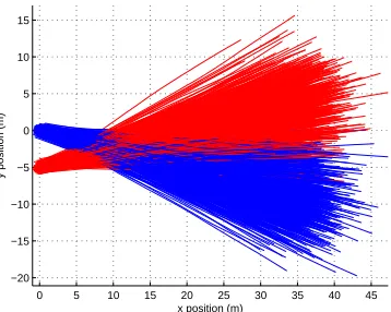
Figure 2: Scenario of the simulations: (a) Target trajectories fordx =

6 m. Each target is identified at the beginning of its trajectory by a label. The trajectories have an asterisk to indicate the target position every ten time steps. (b) Distance between targets against time fordx= 0 mand

dx= 6 m.

posterior PDF has an ever-increasing number of components so we use the joining algorithm in [28] to control the number of components of the mixture. With this algorithm, before the targets get close to each other, the average number of posterior mixture components is one fordx= 0m anddx= 6m. After they separate, it is two.

The averaged CLP and SLMP against time for dx = 0m and dx = 6 m using 1000 Monte Carlo runs are shown in Figure 3. The CLP can be obtained in closed-form and the SLMP is approximated using Monte Carlo integration with 20000 samples. For dx = 0 m, the CLP at the end of the simulation is approximately 0.5 for all the estimators in all Monte Carlo runs. This means that we do not know which estimate corresponds to target 1 and target 2. It should be noted that once the CLP is 0.5, it does not convey any new information. However, the SLMP is always meaningful. As of time step 60, the CLP remains unchanged but the SLMP indicates that the multitarget estimates at consecutive times are (optimally) linked with probability 1. The interpretation is that the targets are now separated enough such that the tracks after this time step belong to the same target with probability one although the association with the tracks before

10 20 30 40 50 60 70

0 0.1 0.2 0.3 0.4 0.5 0.6 0.7 0.8 0.9 1

Time step

E1−CLP E2−CLP E3−CLP E1−SLMP E2−SLMP E3−SLMP E1−CPSLMP E2−CPSLMP E3−CPSLMP

(a)

10 20 30 40 50 60 70

0 0.1 0.2 0.3 0.4 0.5 0.6 0.7 0.8 0.9 1

Time step

E1−CLP E2−CLP E3−CLP E1−SLMP E2−SLMP E3−SLMP E1−CPSLMP E2−CPSLMP E3−CPSLMP

(b)

Figure 3: Correct labelling probabilities and sequential linked multitrack probabilities against time a)dx = 0m b) dx = 6m. In the legend,

CPSLMP stands for the cumulative product of SLMP.

the target crossing is unknown. E3 has a higher probability that two consecutive estimates are linked. This is because it maximises the SLMP. Fordx= 6m, the CLP at the end of the simulation is different for the estimators as the posterior is not permutation invariant. E1 and E2 have the highest probability of correct labelling.

In general, if we are interested in determining where target 1 and target 2 are, we should use E2. However, if we are more interested in building (optimally) connected tracks sequentially with minimum jitter, it is better to use E3. This is illustrated in Figure 4 where the resulting tracks of the estimators for four time steps are plotted for an exemplar run (dx = 0 m). As E3 maximises the SLMP, the resulting four-time-step tracks are more reasonable. E1 and E2 show a jump in the linking of target state estimates. This behaviour happens often as the averaged cumulative product of the SLMPs over the time steps 51, ...,54considered in Figure 4 are, using the results shown in Figure 3 (a): 0.37 for E1, 0.48 for E2 and 0.71 for E3. These results indicate that E3 provides the best tracks, in the sense of minimising switches, followed by E2 and then E1.

B. Process and measurement noise analysis

315 320 325 330 335 340 345 350 365

370 375 380 385 390 395 400

x position (m)

y position (m)

(a)

315 320 325 330 335 340 345 350 365

370 375 380 385 390 395 400

x position (m)

y position (m)

(b)

Figure 4: Track formation for (a) E1 and E2, which have the same output in this exemplar run, (b) E3. The blue circles represent the true target states at time steps k ∈ {51,52,53,54}. The true target states that belong to the same target are linked by a blue line. The red crosses indicate the target state estimate for a target. The black crosses indicate the target state estimate for the other target. The red and black lines indicate how the target state estimates are linked to form tracks. E3, which maximises the SLMP, provides more reasonable tracks than E1 and E2.

measurement noise parameters. The prior PDF at time 0 is

π0 X0=N x01;x01,P0

N x02;x02,P0

where x0₁ = [0,4,0,−1]T, x0₂ = [0,4,−5,1]T and P0 is a diagonal matrix whose entries are 0.1 with international system units. The number of time steps in the trajectory is 18 and

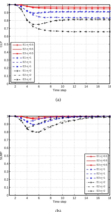
τ = 0.5s. In order to provide a more general analysis than in the previous case that only focused on a particular trajectory, we generate a new multitarget trajectory in each Monte Carlo run.

First, we setσr= 1 mand evaluate the CLP and SLMP for

σu ∈ {0.1,1,10} m/s3/2. To indicate what the trajectories generated from this dynamic model look like, we plot the trajectories used for σu = 0.1 m/s3/2 in Figure 5. The CLP and SLMP against time averaged over all Monte Carlo runs are shown in Figure 6. Forσu= 0.1 m/s3/2, CLP and SLMP are nearly one at all time steps. However, as σu increases, CLP decreases. This implies that it gets more and more difficult to label the multitarget state estimates properly as

0 5 10 15 20 25 30 35 40 45

−20 −15 −10 −5 0 5 10 15

x position (m)

y position (m)

Figure 5: Target trajectories in each Monte Carlo run for σu =

0.1 m/s3/2_{. Target one trajectories are shown in blue and target two}

trajectories in red.

the process noise increases. The SLMP gets also lower asσu increases and the minimum of the SLMP is attained earlier for σu = 10 m/s3/2 than σu = 1 m/s3/2. This is due to the fact that with higher process noise, the targets are likely to get closer together earlier. It should be noted that SLMP for all

σu and all estimators is nearly one as of time step 10. This means that the tracks formed as from this time step belong to the same targets with probability close to one. We want to remark that this information is not contained in the posterior densityπk_{(·)but inπ}k:k+1_(·)

Now, we set σu = 1 m/s3/2 and evaluate the CLP and SLMP forσr∈ {0.5,1,2}(m). The CLP and SLMP against time averaged over all Monte Carlo runs are shown in Figure 7. For σr = 0.5 m, CLP and SLMP are approximately one at all time steps, which indicate that the built tracks belong to the same targets with probability approximately one. As happened with the process noise, performance deteriorates as

σr increases. This is because the sensor has less capability to separate the states of the two targets so they get mixed up more easily. As expected, the SLMP is always higher for E3 than for E1 and E2 in all simulations.

VII. CONCLUSIONS

In this paper, we have presented an analysis on how we can build optimal tracks from the Bayesian point of view. We have proposed two alternatives. The first method takes the customary approach of labelling the states and finding the best labelling of the multitarget estimate in the MSLOSPA sense (with small α). The second method does not require the labelling of the state and builds tracks by labelling the current multitarget state estimate to maximise the probability that is optimally linked with the multitarget state estimate at the previous time step, i.e., it minimises track jittering. The first approach shows some important drawbacks after the targets have moved in close proximity for a long time and then separated. The second approach does not have this drawback and only requires knowledge of the RFS posterior density.

2 4 6 8 10 12 14 16 18 0

0.1 0.2 0.3 0.4 0.5 0.6 0.7 0.8 0.9 1

Time step CLP E1 σu=0.1

E2 σu=0.1 E3 σu=0.1

E1 σu=1 E2 σu=1

E3 σu=1

E1 σu=10

E2 σu=10

E3 σu=10

(a)

2 4 6 8 10 12 14 16 18

0 0.1 0.2 0.3 0.4 0.5 0.6 0.7 0.8 0.9 1

Time step

SLMP E1 σu=0.1

E2 σu=0.1

E3 σu=0.1

E1 σu=1

E2 σu=1 E3 σu=1

E1 σu=10 E2 σu=10

E3 σu=10

(b)

Figure 6: CLP and SLMP against time usingσr= 1 m. Asσuincreases,

performance deteriorates.

build tracks in a sound, well-defined fashion. Second, we can in principle modify classic algorithms like MHT such that they provide jitter-free tracks based on first principles. In general, as explained in the paper, multiple target tracking algorithms should consider exploiting the advantage of only requiring the RFS posterior density or the RFS trajectory posterior in the smoothing problem to build tracks.

An interesting line of future research is to generalise this analysis to a variable and unknown number of targets.

APPENDIXA

In this appendix, we prove why Definition 1 denotes the optimal labelling of a target. To do so, we use the random set notation as it explicitly includes the labels. The true labelled multitarget state set is

Xk=

h

xk₁T,1i T

,h xk₂T,2i T

, ...,h xk_tT, ti

T

(29) where we have assumed that the true labels are [1, ..., t]T without loss of generality.

A labelled multitarget state set estimate is

ˆ

Xk=

_h

ˆ

xk₁T

,ˆl1

iT

,h ˆxk₂T

,ˆl2

iT

, ...,h xˆk_tT

,ˆlt

iT

(30)

2 4 6 8 10 12 14 16 18

0 0.1 0.2 0.3 0.4 0.5 0.6 0.7 0.8 0.9 1

Time step CLP E1 σr=0.5

E2 σr=0.5 E3 σr=0.5

E1 σr=1 E2 σr=1

E3 σr=1

E1 σr=2

E2 σr=2

E3 σr=2

(a)

2 4 6 8 10 12 14 16 18

0 0.1 0.2 0.3 0.4 0.5 0.6 0.7 0.8 0.9 1

Time step

SLMP E1 σr=0.5

E2 σr=0.5

E3 σr=0.5

E1 σr=1

E2 σr=1 E3 σr=1

E1 σr=2 E2 σr=2

E3 σr=2

(b)

Figure 7: CLP and SLMP against time usingσu= 1 m/s3/2. Asσr

increases, performance deteriorates.

where the label vector estimate hˆl1,ˆl2, ...ˆlt

iT

can be any

permutation of[1, ..., t]T.

Definition 6. The optimal labellingφ˜0=hφ˜0₁, ...,φ˜0_ti

T of the labelled multitarget state set estimate is the label vector that minimises the LOSPA distance between (29) and (30):

˜

φ0=φl?: l? = arg min

l∈{1,...,t!}

d

Xk,

_h

ˆ

xk₁T

, φl,1

iT

, ...,h xˆk_tT

, φl,t

iT

= arg min l∈{1,...,t!}

min i∈{1,...,t!}





t

X

j=1

bpxkj,xˆkφi,j

+αpδhj−Γφ_i(φl)j

ii

(31)

whereΓφi(φl)j is thejth component of vector Γφi(φl). In the following we prove that Definitions 1 and 6 are equivalent, i.e., φ˜ = ˜φ0. We make the change of indices (i

is changed byn) such that

φ_n = Γφ_i(φl) (32)

which implies that

φ_i= Γφ_n φ−l 1

whereφ−_l1is the vector that indicates the inverse permutation of φ_l. Then, (31) becomes

l?= arg min l∈{1,...,t!}

min n∈{1,...,t!}

  t X j=1 bp

xk_j,Γ_φ−1

l ˆ Xk φn,j

+αpδ[j−φn,j]

= arg min l∈{1,...,t!}

dXk,Γ_φ−1

l

ˆ

Xk

= arg min l∈{1,...,t!}

dΓφ_l Xk

,Xˆk.

We get thatφ˜ = ˜φ0 using (2).

APPENDIXB

In this appendix, we prove Lemma 2. We define vectorφ?= [φ?₁, ..., φ?_t]T as

φ?=φ_i?: i?= arg min i∈{1,...,t!}

  1 t t X j=1

bpˆxk_j,xk_φ

i,j   1/p . (34) In the following, we show that φ? = ˜φ where φ˜ is the optimal labelling of Xˆk_{. Using (2), we can write}

˜

φ=φ_l?: l? = arg min

l∈{1,...,t!}

dXˆk,Γφ_l Xk

= arg min l∈{1,...,t!}

min i∈{1,...,t!}





t

X

j=1

bpxˆkj,Γφ_l Xk

φi,j

+αpδ[j−φi,j] (35) whereΓφ_l Xk

φi,j denotes the state vector of targetj in the

ith permutation of the multitarget state vector Γφl X k

. Let

φ?_nn∈ {1, ..., t!}denote the permutations of vectorφ?, which is given by (34). We can write (35) as

˜

φ=φ?_n?: n? = arg min

n∈{1,...,t!}

dXˆk,Γφ? n X

k

= arg min n∈{1,...,t!}

min i∈{1,...,t!}





t

X

j=1

bpxˆk_j,Γφ? n X

k

φi,j

+αpδ[j−φi,j]

.

The argument of the minimum (in variable i) of the first term isolated is a function of nand is denoted as i?

1(n)and the argument of the minimum (in variablei) of the second term isolated is i?

2(n) = 1 regardless ofn. If there existsn∗ such that the two arguments of the minima coincide, i.e.,i?₁(n∗) = 1then, the whole expression is minimised andn∗is obtained. For n= 1, the multitarget state vectorΓφ?

n X k

is ordered according toφ?(asφ?1=φ

?

) and, therefore, the argument of the minimum of the first term is i?(1) = 1 because of (34). Consequently, φ˜ =φ?.

APPENDIXC

In this appendix, we prove Equation (6). Using (5), we get

MSLOSPAXˆk

= Ehd2Xk,Xˆki

= ˆ

1

tl∈{min1,...,t!} 



t

X

j=1

b2xk_j,ˆxk_φ

l,j

+α2δ[j−φl,j]





πk Xk

dXk

= ˆ

S1(Xˆk)

1

t

t

X

j=1

b2xk_j,xˆk_φ1,jπk XkdXk

+1 t t! X i=2 ˆ

Si(_Xˆk₎ min l∈{1,...,t!}

t

X

j=1

h

b2xk_j,xˆk_φl,j+α2δ[j−φl,j]iπk XkdXk

It is met that

min l∈{1,...,t!}

t

X

j=1

h

b2xk_j,ˆxk_φ

l,j

+α2δ[j−φl,j]

i ≤ t X j=1 h

b2xkj,ˆxkφi,j

+α2δ[j−φi,j]i

for Xk _{∈ S} i

ˆ

Xk _{and the inequality is tight for α → 0} because of (3). Then,

MSLOSPAXˆk

≤ ˆ

S1(Xˆk)

1

t

t

X

j=1

b2xk_j,ˆxk_φ1,jπk Xk

dXk

+1 t t! X i=2 ˆ

Si(_Xˆk₎ t

X

j=1

h

b2xk_j,ˆxk_φi,j+α2δ[j−φi,j]i

πk Xk

dXk

= MSOSPAXˆk+ MLECXˆk

whereMLECXˆk_{is the mean labelling error cost (MLEC)} of the estimateXˆk_{, see (8), andMSOSPAX}ˆk_{is the mean} square OSPA distance of the estimate Xˆk_{, see (7).}

APPENDIXD

In this appendix, we prove (13). We make the change of variables Ym _{= Γ}

φ_i(Xm)

Xm_{= Γ}−1

φi (Y

m_{) in each} integral in (12) noting that

X0:k ∈ Li

ˆ

X0:k←→Y0:k∈ L1

ˆ

X0:k (36)

because

dXˆm,Γφ_i(Xm)

< dXˆl,Γφ_l(Xm)

l6=i, m∈ {0, ..., k} ←→dXˆm,Ym< dXˆl,Γφ_l(Ym)

Then, (12) becomes

P0:k_ˆ X0:k=

t!

X

i=1 ˆ

Li(Xˆ0:k₎

π0:k X0:k

dX0:k

= t!

X

i=1 ˆ

L1(Xˆ0:k)

π0:kΓ−_φ1 i X

0:k

dX0:k

= ˆ

L1(Xˆ0:k)

ˇ

π0:k

x0:k₁ ,x0:k₂ , ...,x0:k_t dX0:k (37)

where the RFS density over the trajectories

ˇ

π0:k x0:k

1 , ...,x0:kt is given by (14). APPENDIXE

In this appendix we prove (22). The RFS trajectory posterior density from k tok+ 1 can be written as

ˇ

πk:k+1 xk:k+1₁ , ...,xk:k+1_t

= t!

X

i=1

πk:k+1 Γφ_i Xk:k+1

= t!

X

i=1 1

ρi

` zk+1Γφ_i Xk+1

f Γφi X k+1

Γφi X

k _πk _Γ

φi X k

(38)

where

ρi= ˆ

` zk+1Γφ_i Xk+1 f Γφ_i Xk+1 Γφ_i Xk

πk Γφ_i Xk

dXk:k+1. (39)

We apply a change of variables in (39) using the function Γ−_φ1

i (·)as in Appendix D. Under Assumption A1, we can use (18) and (19), and we get:

ˇ

πk:k+1

xk:k+1₁ , ...,xk:k+1_t

=

Pt!

i=1` z k+1

Xk+1

f Xk+1

Xk

πk _Γ

φ_i Xk

´

`(zk+1<sub>|X</sub>k+1<sub>)f(X</sub>k+1<sub>|X</sub>k<sub>)π</sub>k<sub>(X</sub>k<sub>)dX</sub>k:k+1 = ` z

k+1

Xk+1

f Xk+1

Xk

ˇ

πk xk

1, ...,xkt ´

`(zk+1<sub>|X</sub>k+1<sub>)f(X</sub>k+1<sub>|X</sub>k<sub>)π</sub>k<sub>(X</sub>k<sub>)dX</sub>k:k+1 =` z

k+1

Xk+1

f Xk+1Xk

ˇ

πk xk1, ...,xkt

ρ

(40)

where the normalising constantρis given by (23). Substituting (40) into (21), we get

P_ik:k+1=1/ρ

ˆ

L1(Xˆki:k+1)

` zk+1

X

k+1

f Xk+1Xk

ˇ

πk

xk₁, ...,xk_t dXk:k+1.

REFERENCES

[1] S. S. Blackman, “Multiple hypothesis tracking for multiple target tracking,”IEEE Aerospace and Electronic Systems Magazine, vol. 19, no. 1, pp. 5–18, Jan. 2004.

[2] T. Fortmann, Y. Bar-Shalom, and M. Scheffe, “Sonar tracking of multiple targets using joint probabilistic data association,” IEEE Journal of Oceanic Engineering, vol. 8, no. 3, pp. 173 –184, Jul. 1983.

[3] R. P. S. Mahler,Statistical Multisource-Multitarget Information Fusion. Artech House, 2007.

[4] P. Braca, S. Marano, V. Matta, and P. Willett, “Asymptotic efficiency of the PHD in multitarget/multisensor estimation,” IEEE Journal of Selected Topics in Signal Processing, vol. 7, no. 3, pp. 553–564, 2013. [5] W. Koch and F. Govaers, “On accumulated state densities with applica-tions to out-of-sequence measurement processing,”IEEE Transactions on Aerospace and Electronic Systems, vol. 47, no. 4, pp. 2766–2778, 2011.

[6] A. F. García-Fernández, J. Grajal, and M. R. Morelande, “Two-layer par-ticle filter for multiple target detection and tracking,”IEEE Transactions on Aerospace and Electronic Systems, vol. 49, no. 3, pp. 1569–1588, July 2013.

[7] W.-K. Ma, B.-N. Vo, S. Singh, and A. Baddeley, “Tracking an unknown time-varying number of speakers using TDOA measurements: a random finite set approach,”IEEE Transactions on Signal Processing, vol. 54, no. 9, pp. 3291–3304, Sept. 2006.

[8] B. T. Vo and B. N. Vo, “Labeled random finite sets and multi-object conjugate priors,” IEEE Transactions on Signal Processing, vol. 61, no. 13, pp. 3460–3475, July 2013.

[9] A. F. García-Fernández, “Detection and tracking of multiple targets using wireless sensor networks,” Ph.D. dissertation, Universidad Politécnica de Madrid, 2011. [Online]. Available: http://oa.upm.es/9823/ [10] H. Blom, E. Bloem, Y. Boers, and H. Driessen, “Tracking closely spaced targets: Bayes outperformed by an approximation?” in11th International Conference on Information Fusion, July 2008, pp. 1–8.

[11] M. Guerriero, L. Svensson, D. Svensson, and P. Willett, “Shooting two birds with two bullets: How to find minimum mean OSPA estimates,” in13th Conference on Information Fusion, July 2010, pp. 1–8. [12] D. Schuhmacher, B.-T. Vo, and B.-N. Vo, “A consistent metric for

performance evaluation of multi-object filters,” IEEE Transactions on Signal Processing, vol. 56, no. 8, pp. 3447–3457, Aug. 2008. [13] D. F. Crouse, P. Willett, and Y. Bar-Shalom, “Developing a real-time

track display that operators do not hate,”IEEE Transactions on Signal Processing, vol. 59, no. 7, pp. 3441–3447, July 2011.

[14] B. Ristic, B.-N. Vo, D. Clark, and B.-T. Vo, “A metric for performance evaluation of multi-target tracking algorithms,” IEEE Transactions on Signal Processing, vol. 59, no. 7, pp. 3452–3457, July 2011. [15] A. F. García-Fernández, M. R. Morelande, and J. Grajal, “Particle

filter for extracting target label information when targets move in close proximity,” in 14th International Conference on Information Fusion, 2011, pp. 795–802.

[16] H. Blom and E. Bloem, “Permutation invariance in Bayesian estimation of two targets that maneuver in and out formation flight,” in 12th International Conference on Information Fusion, July 2009, pp. 1296– 1303.

[17] ——, “Decomposed particle filtering and track swap estimation in tracking two closely spaced targets,” in14th International Conference on Information Fusion, 2011, pp. 787–794.

[18] D. F. Crouse, P. Willett, L. Svensson, D. Svensson, and M. Guerriero, “The set MHT,” in 14th International Conference on Information Fusion, 2011, pp. 2134–2141.

[19] R. Georgescu, P. Willett, L. Svensson, and M. Morelande, “Two linear complexity particle filters capable of maintaining target label probabili-ties for targets in close proximity,” in15th International Conference on Information Fusion, 2012, pp. 2370–2377.

[20] E. H. Aoki, Y. Boers, L. Svensson, P. Mandal, and A. Bagchi, “A Bayesian look at the optimal track labelling problem,” in9th IET Data Fusion Target Tracking Conference, 2012, pp. 1–6.

[21] M. Arulampalam, S. Maskell, N. Gordon, and T. Clapp, “A tutorial on particle filters for online nonlinear/non-Gaussian Bayesian tracking,”

IEEE Transactions on Signal Processing, vol. 50, no. 2, pp. 174–188, Feb. 2002.

[22] D. F. Crouse, P. Willett, M. Guerriero, and L. Svensson, “An approximate minimum MOSPA estimator,” in IEEE International Conference on Acoustics, Speech and Signal Processing, 2011, pp. 3644–3647. [23] M. Baum, P. Willett, and U. Hanebeck, “Calculating some exact

MMOSPA estimates for particle distributions,” in 15th International Conference on Information Fusion, 2012, pp. 847–853.

[24] Ángel F. García-Fernández, M. R. Morelande, and J. Grajal, “Labelled OSPA metric for fixed and known number of targets.” [Online]. Available: http://arxiv.org/abs/1404.3041

[26] L. Svensson, D. Svensson, M. Guerriero, and P. Willett, “Set JPDA filter for multitarget tracking,”IEEE Transactions on Signal Processing, vol. 59, no. 10, pp. 4677–4691, Oct. 2011.

[27] Y. Bar-Shalom, T. Kirubarajan, and X. R. Li,Estimation with Applica-tions to Tracking and Navigation. John Wiley & Sons, Inc., 2001. [28] D. Salmond, “Mixture reduction algorithms for point and extended

ob-ject tracking in clutter,”IEEE Transactions on Aerospace and Electronic Systems, vol. 45, no. 2, pp. 667–686, April 2009.

Ángel F. García-Fernándezreceived the telecom-munication engineering degree (with honours) and the Ph.D. degree from Universidad Politécnica de Madrid, Madrid, Spain, in 2007 and 2011, respec-tively.

He is currently a Research Associate in the De-partment of Electrical and Computer Engineering at Curtin University, Perth, Australia. His main research activities and interests are in the area of Bayesian nonlinear inference and radar imaging.

Mark R. Morelande received the B.Eng. degree in aerospace avionics from Queensland University of Technology, Brisbane, Australia in 1997 and the Ph.D. in electrical engineering from Curtin Univer-sity of Technology, Perth, Australia in 2001. In 2001 he was a Postdoctoral Fellow at the Centre for Eye Research, Queensland University of Tech-nology. From 2002-2005 he was a Research Fel-low at the Cooperative Research Centre for Sensor, Signal and Information Processing, University of Melbourne. He is now a Senior Research Fellow in the Melbourne Systems Laboratory, also at The University of Melbourne. His research interests include non-stationary signal analysis and target tracking with particular emphasis on multiple target tracking and sequential Monte Carlo methods.

Jesús Grajalwas born in Toral de los Guzmanes (León), Spain, in 1967. He received the Ingeniero de Telecomunicación and the Ph.D. degrees from the Technical University of Madrid, Madrid, Spain in 1992 and 1998, respectively.