Simple components, correlated components and an application of statistical shape analysis to consumer and other multivariate data

(1)

Simple Components, Correlated Components and an

Application of Statistical Shape Analysis to Consumer and

other Multivariate Data

Thesis submitted in accordance with the requirements of the University of Liverpool for the degree of Doctor in Philosophy

by

David Stanley Arnold

(2)

Abstract

The interpretation of a principal component analysis can be complicated because the components are linear combinations of possibly many observed variables. A rotation of the principal components can improve the interpretation, however, there are usually still many small non-informative loadings, which taken together account for a signiﬁcant proportion of the observed variation.

Presented is a new computationally efficient method to find simple components using similar criteria to principal components. Simple components are defined to have re-stricted weights that are proportional to the set of integers{0,±1}. This choice ensures that no subjective decision is required as to whether a weight is important, and an in-dividual weight is interpreted in a similar way to a correlation of one, minus one or zero with the component. The algorithm can find solutions for large problems in tractable time and can easily accommodate alternative criteria. An application is proposed that provides a simple component summary of a large data set.

When data is related to an orthogonal basis, these axes represent the maximum sep-aration of information between axes. An approach is developed that finds orthogonal rotations of the principal components so that the sum or the sum of the squared co-variance between a set of components is maximized. This approach can find a group of correlated components that explain a latent trait, and in addition explain different aspects of that trait. Another application is developed where an arbitrary configu-ration of points from a multidimensional scaling or similar method, can be displayed on a parallel coordinate plot so that the number of cross overs between the axes are minimized. This aids the identification of clusters and outliers.

(3)

Acknowledgements

Firstly, I would like to thank Dr Trevor Cox, without whose supervision, encourage-ment, and expertise, I would not have completed this thesis.

Secondly, Unilever Research for the opportunity to study and for providing the ﬁnancial support and access to appropriate data sets.

My colleagues at Unilever Port Sunlight laboratory, for allowing the time and space to complete the work.

In particular I would like to thank Dr Jane Shaw for her encouragement, support, and suggestions, and help with the process of completing the thesis.

(4)

Dedication

(5)

Introduction

Multivariate data consists of more than one observation collected on each object or individual. There are often many variables which are usually correlated with each other and have an error structure that is more complex than in the case of a univariate data set. Also, the number of measured variables can be greater than the number of individual objects on which they are measured, for example data consisting of spectra or from some sensory product tests. Additionally, the measured variables may be of different types or on different scales. Consequently, the analysis, interpretation and quantification of uncertainty in such data is challenging. The high dimensional nature of most multivariate data makes it sparse and difficult to model statistically. Although work has been done on the estimation and hypothesis testing of population parameters, the methods cannot be used routinely and the majority of methods develop tools to explore and visualize the data and understand its structure. These methods can be considered exploratory. The following list highlights some of the questions that are commonly posed for multivariate data and gives examples of some methods. The list is not exhaustive, but is intended to give a flavour of the challenges and approaches commonly used.

1. Can the relationships be understood? This is concerned with obtaining the struc-ture of the data. For example graphical modelling, path analysis and structural equation modelling all try to simplify the interdependencies between variables into a simple map to represent the true relationships. Hypothesis tests can be formulated to determine the likelihood of the relationships.

(9)

examples. In doing this the error structure of models for the data is simpliﬁed.

3. Can observations and/or variables be classified or grouped? Clustering meth-ods such ashierarchical clustering andk-means clustering group observations or variables based on some notion of distance. A discriminant analysis approaches the problem differently and finds boundaries in the multidimensional space in which the data sits, that separates observations into similar groups. Often the boundaries are formed using linear combinations of the variables, but non-linear boundaries can be fitted, for example usingsupport vector machines.

4. Can a useful visualization be obtained? The previous three tasks in themselves produce a visualization of the data. In many cases the high number of variables is an inflated estimate of the true dimensionality of the data. A simple illustration is when the data sits on a straight line on a two dimensional graph. Abiplot rep-resents the relationships between the variables and the individual objects in two or three dimensions. These are particularly valuable when the true dimensional-ity of the data is of low order. The generative topographic map finds a flexible manifold embedded in the high dimensional space which can then be displayed in a small number of dimension, usually two, but preserves the ordering of the objects. Typically this is used to cluster observations in two dimensions. A differ-ent approach is a parallel coordinate plot which displays observations across the variables by representing them by vertical lines. Then relationships and outliers can be more easily identified.

5. Can the variables be regressed? Multiple linear regression and multivariate anal-ysis of varianceare methods where some assumptions are necessary regarding the dependencies and distribution of the variables and are multivariate generalizations of the univariate methods. However, algorithms exist to deal with independent and dependent sets that exhibit multiple correlation. For example, partial least squares ﬁnds linear sums for both the independent and dependent variable sets, and maximizes the covariance between the two sets.

The boundaries between the tasks are soft. There are also special types of multivariate data, such as ordered point sets used to model shape, and multivariate data collected over time. This thesis develops techniques that relate to principal component analysis, factor analysis and statistical shape analysis, with examples given from consumer data from the fast moving goods industry. The following sections of the introduction develop the ideas behind models that postulate a set of hidden variables calledlatent variables

and later introduces statistical shape analysis.

(10)

variables are termedmanifest variables because the latent variables manifest their hid-den relationships through them. However, in the ﬁrst instance, Principal Component Analysis (PCA) is described. PCA ﬁnds weighted sums of the manifest variables which can then be considered latent variables. In the context of PCA these are termed com-ponents. PCA does not conform to the latent variable model framework primarily because it does not have an error model and explains all the variation in the data by its principal components. Later the principal component factor analysis model (FA) is explored where the model is adapted to be a form of the factor model and an error model is introduced. The purpose for outlining both PCA and FA is that this thesis develops ideas which simplify the structure of components and their interpretation or rotate factors to achieve a desired correlation, the main thrust of PCA and FA.

1.1 Principal Component Analysis

Principal component analysis (PCA) is a dimensionality reduction method which seeks a small set of uncorrelated variables that explain as much of the variation present in the data as possible. As an example, consider a questionnaire which canvases respon-dents on their likes and dislikes of a hair conditioner. If seventy questions are posed, inevitably, a lot of information will be shared between the seventy questions and pos-sibly a much smaller set of questions could capture the same information. PCA finds a linear combination of the observed variables that explains the maximum amount of variation possible. This is the first principal component. The next linear combination is then found that explains the next largest amount of variation but is uncorrelated with the first. This is the second principal component. This is repeated until a full set of uncorrelated components are found. It is hoped that the majority of variation explained by these components is captured by the first few components which then give a lower dimensional representation of the data. If the variance explained by this smaller set is large, for example 90% of the total variation, then the true dimensionality of the data is likely to be the cardinality of this smaller set e.g. three or four dimensional.

1.1.1 Derivation of Principal Components

(11)

components can be found in many standard text books, for example Basilevsky (1994), Bartholomew and Knott (1987), Cox (2005), but is outlined here to link to later work in the thesis.

PCA transformsx toy such that

1. yj =a1jx1+a2jx2+. . .+apjxpforj= 1, . . . , p,a′jaj = 1, whereaj = (a1j. . . apj)′

2. corr(yj, yk) = 0 for j̸=k

3. yj’s are labelled so that variances are in descending order, i.e. var (y1)≥var (y2)≥

. . .≥var (yp)

Let the covariance matrix of x be ΣX. The ﬁrst principal component is found by maximizing its variance. Let

V =a′₁ΣXa1−λ1

(

a′₁a1−1

) ,

whereλis a Lagrange multiplier. Diﬀerentiation ofV with respect toa1 gives

∂V ∂a1

= 2ΣXa1−2λ1a1=0, and so

(ΣX −λ1I)a1 =0.

This is a standard eigenvalue problem. The determinant of ΣX −λ1I must be iden-tically zero to obtain a solution. Hence λ1 must be an eigenvalue of ΣX and a1 its corresponding eigenvector. The variance ofy1 is

var (y1) = var

( a′₁x)

= a′₁ΣXa1 = a′₁λ1a1 = λ1a′1a1 = λ1.

Thusλ1 is the largest eigenvalue ofΣX and a1 its corresponding eigenvector. As ΣX is positive deﬁnite all its eigenvalues must be real and greater than zero.

The next component is found in a similar way except that it is required to be uncor-related with the ﬁrst. This imposes an additional constraint on the maximization as cov (y1, y2) =a′1ΣXa2 and must be zero. Then the following is maximized

V =a′₂ΣXa2−λ2

(

a′₂a2−1

)

(12)

whereλ2andµ12are Lagrange multipliers. After diﬀerentiation with respect toa2 and setting to zero,

∂V ∂a2

= 2ΣXa2−2λ2a2−µ12ΣXa1= 0. (1.2) If this is pre-multiplied bya′₁

2a′₁ΣXa2−2λ2a′1a2−µ12a′1ΣXa1 = 0.

Now, a′₁ΣXa2 = 0 and a′1a2 = 0 by the orthogonality constraint, so µ12(a1ΣXa1) = 0⇒µ12= 0. Substituting back into (1.2) gives

2ΣXa2−2λ2a2 = 0 (1.3) or

(ΣX−λ2I)a2= 0. (1.4) Again, the solution is an eigenvalue/eigenvector pair of ΣX and must be the second largest eigenvalueλ2 and its corresponding eigenvector. The variance ofy2 isλ2. If this process is repeated the solutions are thepeigenvectors ofΣX with corresponding eigen-values being the variances. In some cases repeated eigeneigen-values may occur in which case there is not a unique eigenvector associated with each of these. In these circumstances choosing the eigenvectors to be orthogonal to those previously found ensures the pre-vious arguments hold. Taking all the solutions together, let A = (a1,a2, . . . ,ap) and theny =A′x and var (y) =∆Y, where ∆Y = diag (λ1. . . λp). In practice, the pop-ulation covariance matrix ΣX will not be known but can be estimated by the sample covariance matrix.

When the observed variables are not measured on the same scale it can become diﬃcult to interpret the components especially if some of the variables have vastly larger variance, which then dominate the ﬁrst principal component. The correlation matrix can be used instead of the covariance matrix. Unfortunately, there is not a simple relationship between the principal components of a covariance matrix and those of its correlation matrix.

The Spectral decomposition

Obtaining the principal components from multivariate data where the population co-variance matrixΣX is estimated from the sample covariance matrixSX can be viewed as a Spectral Decomposition of SX. The linear transformation A is the matrix which diagonalizes the symmetric positive deﬁnite covariance matrix SX into the sum of its eigenvalue/eigenvector pairs.

SX =A ∆YA′= p

∑

i=1

(13)

The Singular Value Decomposition

The singular value decomposition (SVD) is a convenient way to obtain the principal components. The SVD of the data matrix X is as follows,

X =UΓV′

whereU has columns consisting of the eigenvectors ofX X′ and V the eigenvectors of

X′X. Here Γ is a diagonal matrix of the shared singular values, and are the square root of the corresponding eigenvalues,

Γ=∆12.

1.1.2 Biplots

Biplots are a set of visualisation techniques for multivariate data. If a technique like PCA explains most of the variation in a data set within the first two or three compo-nents, then biplots are a convenient and intuitive way to visualise the lower dimensional representation. The plot of the principal component scores is a graphical display for the observations and a plot of the coefficients of the first principal component against the second is a graphical display of the variables. A biplot displays both on the same axis. Biplots were introduced by Gabriel (1971) and an authoritative monograph on the subject is Gower and Hand (1996). Biplots can represent both continuous and cat-egorical data. Points on the plot represent observations, and then axes are overlayed to represent the variables. Theclassic biplot is obtained by factorizing the data matrix into row (observations) H and column (variable) G matrices. If k is the rank of X

then,

X(N×p)=H(N×k)G(k×p).

Approximating the data by approximating H and G by N ×2 and 2×p matrices respectively,

X ≈H2G2,

then the observations are represented by plotting H2 as points in a two dimensional space, and the variables are represented as axes on the same plot based on thepvectors ofG2.

The matricesHandGare obtained from the singular value decomposition ofX, and then approximatingX with the ﬁrst two singular values, and introducing a parameter

α,

X = UΓV′

X ≈ U2Γ2V2′ ≈ (U2Γα2)

(

V2Γ1₂−α

(14)

with 0≤α≤1. Diﬀerent biplots are obtained by varying α. Then U2Γα2 =H2 is the

N×2 matrix with each row representing an observation ofX andΓ₂1−αV′₂ =G2 is the 2×p vector with each column representing a variable. When α= 1 this is a principal component biplot.

1.1.3 Example PCA

Much work has been done to frame PCA on the sample covariance matrix in an in-ferential setting. However, in this thesis the main purpose of a PCA is to reduce the dimensionality of a set of data and explore relationships. When a high dimensional data set is intrinsically of much lower dimension, plotting the first two or three princi-pal component scores will give a straightforward visual representation of what the data looks like. This is because the first q principal components minimize the sum of the squared projection errors for each data point onto the subspace spanned by theq PCs. According to Jolliffe (2002) there are four areas to consider.

1. Which principal components are of interest

2. How many variables to keep

3. Are components considered sequentially or simultaneously

4. What is meant by ‘approximating’ the components

When considering which components are of interest, often the first q components are taken based on the proportion of variance explained in the data or a scree plot is used to see where the change in the variance explained flattens off. Alternatives, are to consider the eigenvalues with unequal variance as judged by a hypothesis testing procedure or by using a cross-validation process; again Jolliffe is an authoritative text. With an analysis on the sample covariance matrix, near zero eigenvalues may indicate the presence of linear dependencies between the variables which can then be dealt with (by removing a variable for instance). Linear dependencies and constant relationships between variables will show on the last principal components and often as large loadings on these. Therefore it is important also to look at the last principal components as a diagnostic aid.

(15)

PCA considers components sequentially, but in so doing is still optimal in terms of the variation explained. However, if components are desired which are more interpretable, then a sequential approach will probably not give a globally optimal solution for the chosen objective. This is linked to the final point of what is meant by approximating a set of components. However, in this thesis, approximating PCA is not the goal, but rather to find an interpretable set of components based on a defined simple set of loadings {-1, 0, 1}.

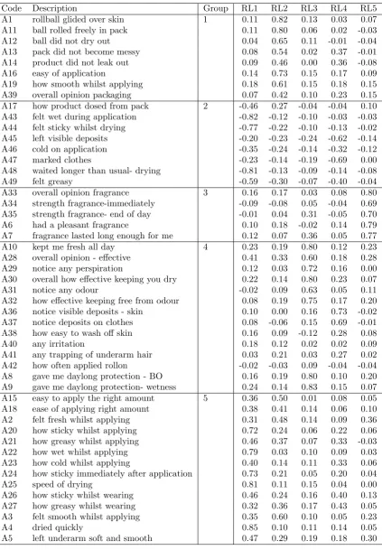
The following example, of what might be termed a standard PCA, is taken from a sensory test where subjects were asked to access deodorant products by answering a questionnaire. There were 49 sensory questions scored on an ordinal scale, coded as 1 to 5, which represented a strong disagreement to a strong agreement. Additionally, there is a question scoring overall opinion on a 1 to 7 scale. Three test products were used, each subject assessed one of the products. There are 450 subjects giving 150 assessments per product. The attribute descriptors are listed in Table 1.2. One requirement of an analysis is to determine how the sensory data inﬂuences overall opinion. The correlation or regression of the principal components with overall opinion can be used to identify possible drivers. The data is taken as a whole in order to understand how the sensory questions relate to the overall opinion score. It is hoped that the products in the test will span the sensory space as measured by the questionnaire.

A PCA on the correlation matrix was used with overall opinion omitted, so that its re-lationship with the principal components of the sensory variables could be investigated later. The use of the correlation matrix simpliﬁes the interpretation of the loadings, which are scaled as in Section 1.3.6 , and so also represent the actual correlation of the variables with the principal components.

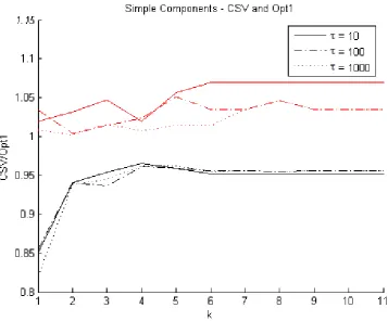
Figure 1.1 is a scree plot, which shows the eigenvalues obtained from the analysis. There is a flattening off of the curve after the fifth eigenvalue. However, these five

(16)

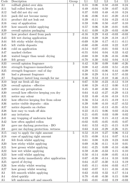
only explain 52% of the total variation, but this is typical of this type of sensory data. In fact, a good low dimensional representation of these data is not obtained with a PCA. However, these may still be useful to interrogate the data graphically. Table 1.2 show the loadings for the five principal components. An hierarchical cluster analysis on the five loading vectors helped to identify five groups of variables, which differentiate across the five vectors. The groups are listed in Table 1.1. For example the Drying and Deposits have high negative loadings on L1. L1 is capturing the contrast between positive and negative drivers of overall opinion. Indeed the subject scores for L1 are highly correlated with overall opinion which was left out of the PCA. Unfortunately, only this first and the second loading vectors are easy to label. It is useful to be able to identify labels for all the loading vectors. To make sense of the loading vectors, it is necessary to make subjective decisions regarding the importance of individual loadings, and to interpret across loading vectors. i.e. each loading vector cannot individually be labelled. The interpretation of the loading vectors and individual loading values (in this case also correlation), is not trivial. Cadima and Jolliffe (1995, 2001) explore

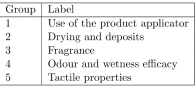
Group Label

1 Use of the product applicator 2 Drying and deposits

3 Fragrance

[image:16.595.223.418.332.418.2]

4 Odour and wetness eﬃcacy 5 Tactile properties

Table 1.1: Variable groups identiﬁed from the ﬁve principal component loading vectors

issues of interpreting the loadings and correlations. Apart from the first component where the variables with the largest absolute loadings are the most highly correlated, it is not possible to judge the correlation of a particular variable with subsequent components by purely examining the size of the loadings. When the correlation of a variable with a component is compared against the corresponding loadings, the size of a loading does not always give a good indication of the correlation of that variable with the principal component. In fact, the only time this is guaranteed to be the case is with the first principal component in which case the largest absolute loadings will have the largest correlations. Consequently, variables with high loadings may not be correlated as strongly as would appear and, conversely, variables with lower absolute loadings may be more highly correlated. This can also be the case when looking across component loadings where a given variable can have similar loadings but have very different correlations.

(17)

[image:17.595.117.544.93.698.2]

Code Description Group L1 L2 L3 L4 L5 A1 rollball glided over skin 1 0.55 0.06 0.58 -0.03 0.24 A11 ball rolled freely in pack 0.49 -0.04 0.59 -0.07 0.25 A12 ball did not dry out 0.37 0.03 0.48 -0.10 0.24 A13 pack did not become messy 0.46 -0.06 0.41 -0.20 -0.13 A14 product did not leak out 0.39 -0.11 0.34 -0.23 -0.13 A16 easy of application 0.59 0.06 0.50 -0.07 0.10 A19 how smooth whilst applying 0.57 0.06 0.38 -0.01 0.05 A39 overall opinion packaging 0.41 0.09 0.29 -0.03 -0.08 A17 how product dosed from pack 2 -0.16 0.29 0.43 -0.03 -0.03 A43 felt wet during application -0.64 0.39 0.28 -0.18 -0.17 A44 felt sticky whilst drying -0.69 0.38 0.17 -0.11 -0.11 A45 left visible deposits -0.60 -0.08 -0.03 0.22 0.37 A46 cold on application -0.54 0.07 -0.01 0.03 0.13 A47 marked clothes -0.55 0.04 0.04 0.33 0.42 A48 waited longer than usual- drying -0.68 0.38 0.26 -0.16 -0.06 A49 felt greasy -0.70 0.30 0.02 0.04 0.13 A33 overall opinion fragrance 3 0.42 0.30 0.09 0.60 -0.26 A34 strength fragrance-immediately 0.08 0.42 -0.03 0.51 -0.23 A35 strength fragrance- end of day 0.29 0.55 -0.06 0.44 -0.09 A6 had a pleasant fragrance 0.38 0.29 0.14 0.57 -0.33 A7 fragrance lasted long enough for me 0.46 0.53 -0.10 0.46 -0.15 A10 kept me fresh all day 4 0.67 0.50 -0.23 -0.12 0.18 A28 overall opinion - effective 0.80 0.28 -0.12 0.00 0.12 A29 notice any perspiration 0.45 0.40 -0.30 -0.31 0.14 A30 overall how effective keeping you dry 0.64 0.43 -0.27 -0.29 0.13 A31 notice any odour 0.33 0.48 -0.16 -0.18 0.15 A32 how effective keeping free from odour 0.56 0.54 -0.15 -0.19 0.11 A36 notice visible deposits - skin 0.39 0.00 -0.10 -0.37 -0.52 A37 notice deposits on clothes 0.34 0.01 -0.13 -0.35 -0.51 A38 how easy to wash off skin 0.22 -0.15 0.06 0.02 -0.24 A40 any irritation 0.21 -0.05 0.03 0.09 0.02 A41 any trapping of underarm hair 0.23 0.00 0.15 -0.12 -0.16 A42 how often applied rollon -0.02 0.05 -0.05 -0.05 0.07 A8 gave me daylong protection - BO 0.61 0.53 -0.21 -0.15 0.19 A9 gave me daylong protection- wetness 0.63 0.43 -0.29 -0.26 0.21 A15 easy to apply the right amount 5 0.52 -0.18 0.27 0.06 0.12 A18 ease of applying right amount 0.55 -0.08 0.14 0.07 0.14 A2 felt fresh whilst applying 0.61 0.08 0.23 0.23 0.03 A20 how sticky whilst applying 0.69 -0.36 -0.11 0.10 0.01 A21 how greasy whilst applying 0.61 -0.25 0.09 -0.10 -0.06 A22 how wet whilst applying 0.59 -0.38 -0.33 0.15 0.10 A23 how cold whilst applying 0.50 -0.14 -0.08 -0.05 -0.14 A24 how sticky immediately after application 0.67 -0.38 -0.14 0.10 0.03 A25 speed of drying 0.64 -0.37 -0.30 0.13 0.19 A26 how sticky whilst wearing 0.65 -0.11 -0.04 -0.03 -0.17 A27 how greasy whilst wearing 0.62 -0.07 0.11 -0.16 -0.16 A3 felt smooth whilst applying 0.63 -0.03 0.32 0.17 0.14 A4 dried quickly 0.70 -0.40 -0.30 0.15 0.08 A5 left underarm soft and smooth 0.65 -0.01 -0.02 0.19 -0.03

(18)

weighted averages or contrasts of the remaining loadings. Firstly, together a large num-ber of small loadings will account for a significant proportion of the observed variation and, secondly, approximating components in this way can lead to misinterpretation due to these truncated components poorly approximating the original components. A different subset of the same size may provide a better approximation. Also, cor-relations between individual variables and principal components are not appropriate, except when judging the adequacy of single-variable approximations. In fact, except for a single variable approximation, finding a subset of variables that closely approximates the original requires a combinatorial search. Cadima and Jolliffe recommend measures, and a search strategy to find the best subsets for moderate size problems.

The following ﬂawed approach is often taken in practice. Considering the deodorant data and ignoring the small loadings, general patterns may be observed between the component loadings and the variable groups and these are shown in Table 1.3.

Group Description L1 L2 L3 L4 L5 1 Use of the product applicator + 0 + - +/-2 Drying and deposits - + + +/- +

3 Fragrance + + 0 +

-4 Odour and wetness eﬃcacy + + - - +/-5 Tactile properties + - +/- +/-

+/-Table 1.3: Group structure across the loadings by reducing the weights to the sign of the majority weight in that group on each component

(19)

[image:19.595.151.488.132.474.2]

to be made on whether a particular loading is important or not, and this can lead to more interpretable components.

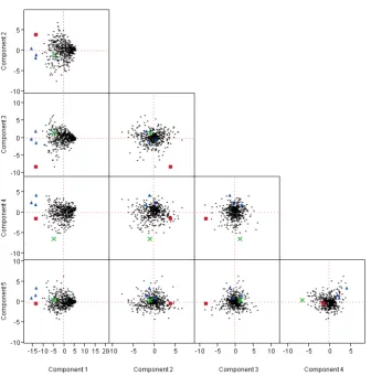
Figure 1.2: A Scatterplot matrix of the principal component scores.

(20)

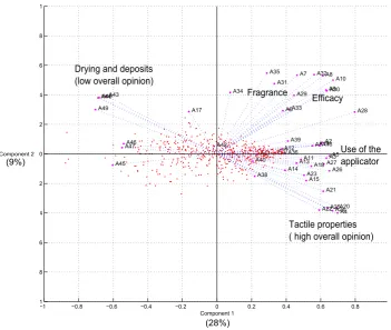
−1 −0.8 −0.6 −0.4 −0.2 0 0.2 0.4 0.6 0.8 −1 −0.8 −0.6 −0.4 −0.2 0 0.2 0.4 0.6 0.8 1 A1A2 A3 A4 A5 A6 A7 A8 A9 A10 A11 A12 A13 A14 A15 A16 A17 A18 A19 A20 A21 A22 A23 A24 A25 A26 A27 A28 A29 A30 A31 A32 A33 A34 A35 A36 A37 A38 A39 A40 A41 A42 A43 A44 A45 A46 A47 A48 A49 Component 1

Drying and deposits (low overall opinion)

Tactile properties ( high overall opinion) Fragrance

Efficacy

Use of the applicator

(28%) (9%)

[image:20.595.146.498.135.432.2]

Component 2

Figure 1.3: A biplot showing the sensory variables on the first two principal compo-nents. Some of variable clusters identified differentiate well on the first two principal components, however, clearly a higher dimensional representation is required as only 37% of the variation is captured by these two components.

Prin1 0.70 Prin2 0.17 Prin3 -0.10 Prin4 0.21 Prin5 0.08

(21)

[image:21.595.220.417.76.295.2]

Figure 1.4: A plot showing the overall opinion scores against the ﬁrst principal compo-nent scores for the deodorant data

1.2 Multidimensional Scaling

PCA can give a low dimensional map of objects which sit in high dimensional space. However, there is a broader set of methods called Multidimensional Scaling (MDS)

which take a set of dissimilarities (or similarities) between objects and then ﬁnd a conﬁguration of points in a low dimensional space where each point represents one of the objects, and is such that distances between pairs of points in the space match the dissimilarities between the corresponding pairs of objects or the rank order of distances correspond to the rank order of dissimilarities; matching being that which is best achievable in some sense. An authoritative monograph on the subject is Cox and Cox (2000).

MDS methods can be split into metric and non-metric scaling. For metric scaling, the dissimilarities{δrs}between pairs ofnobjects are represented directly by distances {drs} between pairs of corresponding points in the conﬁguration.

One type of metric scaling isClassical Scaling. Very brieﬂy, letG=[−1₂d2_rs]and this is centred to giveB, i.e. B=HGHwhereHis the centring matrix. Now B=X X′ is the inner product matrix (corrected for translation so that its centroid is at the origin) and is positive semi-deﬁnite with p non-zero eigenvalues and n−p zero eigenvalues. The spectral decomposition of B (see 1.1.1) is B =U∆U′ and taking thep non-zero eigenvalues and corresponding eigenvectors so that

(22)

then the coordinates are recovered from

X =Up∆

1 2 p.

It can be shown that if Euclidean distance is used as a measure of dissimilarity then classical scaling is equivalent to PCA. In this case the points on the map are projected onto the principal axes.

In general, metric scaling will often minimize a loss function of the form

∑

r<sw_∑rs(drs−δrs)2 r<sδrs

,

sometimes called astrain. An example is a Sammon map (Sammon, 1969).

In a non-metric scaling, the magnitude of the distances between pairs of points no longer approximate the corresponding magnitude of the original dissimilarities. In-stead, the rank orders are matched as well as possible. One approach to obtain a representation of the rank order is the minimization of Kruskal’s (1964) loss function of the form

S=

√ S∗ T∗,

whereS∗ =∑n_r_<_s

(

drs−dˆrs

)2

and T∗ =∑_r_<_sd2_rs is a normalizing term. S is termed the Stress function and ˆdrs are called disparities. The set of disparities {dˆrs} are obtained by ﬁtting a monotone least squares regression of the{drs}on the dissimilarities {δrs}. An iterative algorithm is used to minimize the stress.

A useful application of later work in the thesis is the convenient display of three dimensional or higher MDS configurations. In the case of non-metric scaling the axes are arbitrary and so can be rotated. If the configuration is rotated to maximize the correlation between object coordinates, then this can aid the search for clusters and outliers. In the case of classical scaling the points are projected onto the principal axes and as such have meaning relevant to these. However, rotation to a new set can still be useful to identify clusters and outliers. An application discussed in this thesis is to minimize the number of cross overs in a parallel coordinate plot given a configuration of points obtained from a MDS method. This could be any configuration that can be rotated (See Chapter 3).

1.3 The Latent Variable Model (LVM)

(23)

x

1

x

2

x

3

f

1

f

2

Figure 1.5: The manifest variablesx1, x2, x3are independent of one another conditional on the latent variablesf1, f2.

variables f′ = [f1, . . . , fk], k ≪ p, the general latent variable model usually assumes that the relationships observed between the observed variables are independent given the much smaller set of latent variables. This is the key assumption, that the latent variables produce the relationships between the observed variables. Then the behaviour of the observed variables are essentially random, conditioned on the underlying latent variables. Subsequently, all latent variable models assume that the joint probability distribution of x1, . . . , xp conditioned onf, say Φ(x|f), is such that x1, . . . , xp, given f are independent. If x is continuous then Φ is a density function, but if x is discrete Φ is a set of probabilities. The unconditional density function for x is obtained by integrating the convolution

p(x) =

∫

F

Φ(x|f)h(f)df,

where h(f) is the joint distribution function of f. The conditional probability Φ(x|f) is the mapping from the latent variable space to the data space and includes a noise model to account for random error. It is impossible to infer Φ and h uniquely from

p(x) without making assumptions. Firstly, as the observed variables are independent, conditioned on the latent variables,

Φ(x|f) =ϕ1(x1|f)ϕ2(x2|f). . . ϕp(xp|f).

(24)

1.3.1 The Factor Analysis Model

The key assumption of the factor analysis model is that given a smaller set of latent variables, the manifest variablesx are essentially independent when conditioned on the latent variables. What this infers is that the observed inter-correlations between the observed variables are explained by the latent variable set except for random error. If they are not, then this indicates that a latent variable is missing from the model or the model is not adequate for the data. This is the basis of what is termed R-mode factor analysis. In an R-mode factor analysis the inter-correlations between the observed variables are modelled. A Q-mode factor analysis concerns how the objects relate to one another. The R-mode factor model is now discussed. The model is

x =Γf+e, (1.5)

where x is a column vector containing the p observed variables, f = [f1, . . . , fk]′ rep-resent the k latent variables (k≪p) or common factors,e = [e1, . . . , ep]′ are residual terms andΓ= [γij] is ap×kmatrix of factor loadings. The model postulates that the observed variables are linear combinations of the latent variables and a residual error. For any given observed variable xi,

xi= k

∑

j=1

γijfj+ei. (1.6)

For a data sample X, of nobservations onp variates, the model becomes,

X₍_n_×_p₎ =F₍_n_×_k₎Γ′₍_k_×_p₎+E₍_n_×_p₎. (1.7)

F is the matrix of factor scores, Γ the matrix of factor loadings and E is a matrix of residual or error terms.

1.3.2 Variability in the factor model

From equation (1.5) the complete R-mode factor analysis model for the variance and covariance of the manifest variables is given by

Σ=ΓΦΓ′+Ψ, (1.8)

(25)

variables are uncorrelated then Φ is an identity matrix and (1.8) implies that the variances of the observed variables may be split into two parts as follows,

σii= k

∑

j=1

γ_ij2 +ψii. (1.9)

The ﬁrst term ∑k_j₌₁γ2_ij is called the communality and is the variance that xi shares with the other observed variables through the factors. The covariances of the observed variables are given by

σij = k

∑

r=1

γirγjr (1.10)

and it is only the factors that are involved in these. The matrix of factor loadingsΓis also known as the factor pattern matrix. When standardized factors are uncorrelated then,Φ=I, and then the pattern matrix gives the covariance of the observed variables with the factors,

cov (xi, fj) =γij. (1.11)

1.3.3 Indeterminacy

For a single factork= 1 the model described by (1.5) and (1.8) has a unique solution. However for k > 1 no unique solution exists. To determine a particular solution the factors have to be referred back to a set of basis vectors. These basis vectors may be orthogonal or oblique. If the chosen reference basis is oblique the factors are correlated and a full description of the solution requires both the factor pattern matrixΓand the

factor structure matrix ΓΦ. In which case the coeﬃcients of the pattern matrix are no longer covariances but should be thought of as regression coeﬃcients. The factor modelx =ΓΓ′+Ψ,Φ=I, has pk+p=p(k+ 1) parameters but there arep(p+ 1)/2 variances and covariances inΣ. The model will only be useful if it has less parameters than there are unique elements ofΣ, sop(k+ 1)≤p(p+ 1)/2, i.e. k≤(p−1)/2. In the case of a single factor (k= 1) a unique solution exists up to the sign. The following is an example for p= 3

Σ =



 22 26 36 3 6 10



=

  12

3



 [ 1 2 3 ]+



 10 02 00 0 0 1

 .

(26)

an inﬁnite number of choices forΓ. To illustrate, iff is replaced byRf andΓ byΓR′, whereR is an orthogonal rotation matrix. Then

x =ΓR′Rf+e,

and since R′R = I the model is unchanged by these transformations. Such a trans-formation also leads to the same form for the covariance matrix, since the new factors have a correlation matrix given by

Rﬀ′R′=RΦR′

so that the new factorsRf and new loadingsΓR imply that

Σ= (ΓR′)(RΦR′)(RΓ′) +Ψ,

=ΓΦΓ′+Ψ.

Consequently, the ability of the new factors to account for the variances and covari-ances of the observed variables is exactly equivalent to the original factors. Such a transformation corresponds to a rotation of the factors.

1.3.4 Confirmatory Factor Analysis

In some situations an investigator may wish to fix certain parameters inΓandΨ. This is then termed aconfirmatory factor analysis and this may lead to a unique solution for the free parameters as a rotation would destroy the pattern of the fixed parameters. If the number of fixed parameters are denoted respectively bynΓandnΨ then a necessary

but not suﬃcient condition for a unique solution is

nΓ+nΨ ≥k2.

However, in general it is difficult to give sufficient conditions for uniqueness, since the position of the fixed parameters is also important.

1.3.5 Estimating the Model Parameters

To estimate the parameters, a discrepancy function between the parametrized model covariance matrixΣ(Γ,Ψ) and the unbiased sample covariance matrixSis minimized. Commonly, maximum likelihood is used, but other discrepancy functions are possible, for example, ordinary least squares and generalized least squares. See Everitt for details. The aim is to estimateΓ and Ψso that

(27)

where the hat symbol above a parameter, matrix or vector indicates that it is esti-mated. Here the factors are orthogonal so thatΦ=I. Ifx,f andehave multivariate normal distributions then maximizing the log-likelihood is equivalent to minimizing the discrepancy function

F(S,Σ(Γ,Ψ)) = loge|Σ|+ traceSΣ−1−loge|S| −p

withΣ=ΓΓ′+Ψ. This can be minimized using an iterative procedure suggested by J¨oreskog (see Mardia et al., 1979, for the detail).

1.3.6 Principal Component Factor Analysis

A PCA is primarily a dimensionality reduction technique. However, if the principal componentsy =A x are now considered to be factors then the principal components can be reformulated as a factor analysis model. The model becomes, by multiplying by the inverse of A

x =A′y. (1.12)

If the ﬁrstkcomponents describe the variation in the data that captures the relation-ships between the observed variables, then the remaining components represent the residual variation or random error,e and the model can be written

x =A′_ky_k+e.

These errors are taken to be uncorrelated. In terms of the covariance of x, this gives

Σ = var(A′_ky_k+e)

= var(A′_ky_k)+ var (e) + 2cov(A′_ky_k,e)

= var(A′_ky_k)+Ψ,

assuming cov (A′_ky_k,e) =0. Then

Σ=Γ′ΦΓ+Ψ,

whereΓ=Ak,Φ=∆k and Ψis a diagonal matrix of errors.

The communality ˆhi of theith observed variable is deﬁned across a subset ofkfactors as

ˆ

hi = k

∑

j=1

a2_ji,

(28)

a correlation matrix the variable loadings on the factors reﬂect its correlation with a given factor. The covariance of an observed variable xi with a factoryj is given as

cov (yj, xi) = cov

( yj,

p

∑

k=1

aikyk

)

= p

∑

k=1

aikcov (yj, yk)

= aijvar (yj)

= aijλj

and the correlation is given as

corr (yj, xi) =

aijλj

λ

1 2 j

= aijλ 1 2 j.

So in general

corr (y,x) =A Λ12. (1.13)

1.3.7 Factor Rotation

As mentioned in Section 1.3.3, factors are not unique and any rotation of a factor subset is also a solution. Rotation of a subset of the principal components to a simpler structure will conserve the total variance explained but it becomes more spread between components with either a loss of ortho-normality or the introduction of correlation. What is the best way to choose a solution? One approach is to make factors align more with the original variables, i.e. making a few of the coeﬃcients within factors as large as possible in magnitude, and the rest small. This can be achieved by applying additional constraints on the optimization.

(29)

The Orthogonal Rotation

An orthogonal rotation preserves the orthogonality between all the factors but will induce correlation, unless the factors are standardized by scaling with their standard deviations,∆−12. Avarimax rotation (Kaiser, 1958) is a commonly applied orthogonal rotation. The varimax method searches for a linear combination of a subset of the original factors, such that the sum of the variances of the squared loadings is maximized,

V =

k

∑

j=1

( _p

∑

i=1

a2_ij −1 p

p

∑

i=1

a2_ij

)2

,

with a2_ij being the squared loading of the ith variable on the jth factor, and k the number of factors which are rotated.

There are many orthogonal rotations available, for example others arequartimax and

orthomax rotations. All try to align the new orthogonal axes with the variables. Or-thogonal rotations are commonly used, and will locate orOr-thogonal variable clusters. However, axes that align better with natural variable clusters may better fulﬁll Thur-stone’s criteria (see Section 2.1). Oblique rotations relax the condition that factors must be orthogonal and allow the new axes to take any position in the factor space.

The Oblique Rotation

(30)

This thesis explores factor rotations that preserve orthogonality while maximizing the correlation between the factors. The R-mode factor analysis model can be formulated in two ways; as atrue factor analysis in which factors account for the maximum inter-correlations of the observed variables and principal component factor analysis where factors account for maximum variance. The next section highlights some key ideas around the rotation of principal component factors. This links into the work in later chapters.

1.3.8 Principal Components and Factor Rotation

Orthogonal Rotation of Principal Components

Jolliﬀe (1995) discusses the eﬀects of the orthogonal rotation of principal components and shows why it is not possible to preserve rotated components which are pairwise uncorrelated and/or whose loadings are orthogonal. Consider the mean centred or standardized data sampleX, then its principal components are given by

Y =X U,

using the spectral decomposition of the covariance matrix ofX (Section 1.1.1). Taking the ﬁrst k components and treating the remaining components as residual error, e, a PC factor model can be written

X =YkU′k+e, (1.14)

and the covariance matrix ofX is modelled as

Σ=UkY′kYkU′k+Ψ,

Ψdenoting a diagonal matrix of residual variance. As Yk are principal components,

Y′_kYk=∆k, which is a diagonal matrix of the ﬁrstk eigenvalues ofΣ in descending order of magnitude. Then,

Σ=Uk∆kU′k+Ψ.

Notice that the factors, Yk and the principal component loading vectors are uncorre-lated as U′_kUk =I and Y′kYk =∆k. As mentioned earlier the model is invariant to an orthogonal rotation of the principal axes. Let R be an orthogonal rotation, then

R′R =R R′ =I and the model becomes

X = (YkR)(UkR)′+e

which is equivalent to (1.14). However, the factors will no longer remain uncorrelated, as

(31)

The factor loadings will remain orthogonal,

(UkR)′(UkR) =R′U′kUkR =I.

In practice the factors are usually standardized, which causes the factors to remain uncorrelated after an orthogonal rotation (the loadings become non-orthogonal). This practice is criticized in the literature as standardization eﬀectively stretches the scores to sit on a hypersphere so that any position of the axes will not induce correlation.

To standardize the factors, letZ=Y ∆−12, and the factor model becomes,

X =Zk∆

1 2

kU′k+e and

Σ=Uk∆

1 2

kZ′kZk∆ 1 2

kU′k+Ψ. Now, Z′_kZk =Ik and the factor loadings are Uk∆

1 2

k. So after an orthogonal rotation of the axes, the factors remain uncorrelated as,

(ZkR)′(ZkR) =Ik

but the loadings are no longer uncorrelated, as

(Uk∆ 1 2

kR)′(Uk∆ 1 2

kR) =R′∆kR.

In the literature, if factors are highly correlated this is taken as meaning the factors should really be one single factor. Oblique rotations, will better align with natural vari-able clusters and for this reason are recommended. However, in certain circumstances it may be useful to obtain orthogonal factors which are highly correlated. For example, when groups of correlated components differentiate to describe a latent trait in different ways. Or given a configuration of points from an analysis, for example an MDS, and the axes are arbitrary, it would be useful to rotate the configuration in such a way that the correlation or covariance between the latent variables is maximized, but keeping the axes orthogonal. In this way the latent variables could be displayed on a parallel coordinate plot. The axes remain independent, but the plot becomes easier to interpret as groups differentiate and the number of cross-overs on the plot are minimized. These applications are investigated in Chapter 3.

Oblique Rotation of Principal Components

(32)

Firstly, an oblique rotation relaxes the requirement that the axes are orthogonal, and so ﬁnding oblique axes is more akin to regression. Basilevsky has the detail. If both the variables and factors are standardized to unit length, then, ifG ={g1,g2, . . . ,gk} represents the oblique basis then,

ˆ

Σ=BΦB′+Ψ

and

Φ=G′G

which is the correlation matrix of the oblique axes. B is described in terms of an ordinary least squares projection of the dataX,

B′ = (G′G)−1G′X (1.15)

and so the estimate ofX is

ˆ

X =G B′ =G(G′G)−1G′X =PGX

wherePG is an idempotent, symmetric projection matrix. From (1.15),

ΦB′ =G′X.

G′X is the correlation matrix of the variables and the oblique components, called the matrix of correlation loading coefficients. Bare the regression coefficients and represent the coordinates ofX with respect to the oblique components G. G is not unique and to define the oblique basis a further constraint is required. Criterion such as oblimin

provide this, and in a similar way to the varimax criterion guide the axes position to align with the variables.

Chapter 3 explores the case where axes can be found which remain orthogonal but the induced correlation between factors may provide groups of axes which although correlated, describe diﬀerent aspects of a latent trait.

1.3.9 The Sensory Panel Example Re-visited

(33)

rotated component scores correlate with overall opinion as highly as did the ﬁrst PC, Table 1.6, but a regression model using the new factors will be more interpretable. As mentioned previously, Chapter 2 reviews approaches to deal with the subjective choice of loadings, and a new algorithm is proposed.

Group Description RL1 RL2 RL3 RL4 RL5 1 Use of product applicator +

2 Drying and deposits - -

-3 Fragrance +

4 Odour and wetness eﬃcacy + +

5 Tactile properties + + +

Table 1.5: A subjective interpretation of the loadings on the rotated principal compo-nents

Rotated Factor Correlation with overall opinion

Factor1 0.46

Factor2 0.27

Factor3 0.39

Factor4 0.08

Factor5 0.38

Table 1.6: The correlation of the rotated factor scores with overall opinion for the deodorant data

1.3.10 Other Latent Variable Models

(34)

[image:34.595.119.543.88.698.2]

Code Description Group RL1 RL2 RL3 RL4 RL5 A1 rollball glided over skin 1 0.11 0.82 0.13 0.03 0.07 A11 ball rolled freely in pack 0.11 0.80 0.06 0.02 -0.03 A12 ball did not dry out 0.04 0.65 0.11 -0.01 -0.04 A13 pack did not become messy 0.08 0.54 0.02 0.37 -0.01 A14 product did not leak out 0.09 0.46 0.00 0.36 -0.08 A16 easy of application 0.14 0.73 0.15 0.17 0.09 A19 how smooth whilst applying 0.18 0.61 0.15 0.18 0.15 A39 overall opinion packaging 0.07 0.42 0.10 0.23 0.15 A17 how product dosed from pack 2 -0.46 0.27 -0.04 -0.04 0.10 A43 felt wet during application -0.82 -0.12 -0.10 -0.03 -0.03 A44 felt sticky whilst drying -0.77 -0.22 -0.10 -0.13 -0.02 A45 left visible deposits -0.20 -0.23 -0.24 -0.62 -0.14 A46 cold on application -0.35 -0.24 -0.14 -0.32 -0.12 A47 marked clothes -0.23 -0.14 -0.19 -0.69 0.00 A48 waited longer than usual- drying -0.81 -0.13 -0.09 -0.14 -0.08 A49 felt greasy -0.59 -0.30 -0.07 -0.40 -0.04 A33 overall opinion fragrance 3 0.16 0.17 0.03 0.08 0.80 A34 strength fragrance-immediately -0.09 -0.08 0.05 -0.04 0.69 A35 strength fragrance- end of day -0.01 0.04 0.31 -0.05 0.70 A6 had a pleasant fragrance 0.10 0.18 -0.02 0.14 0.79 A7 fragrance lasted long enough for me 0.12 0.07 0.36 0.05 0.77 A10 kept me fresh all day 4 0.23 0.19 0.80 0.12 0.23 A28 overall opinion - effective 0.41 0.33 0.60 0.18 0.28 A29 notice any perspiration 0.12 0.03 0.72 0.16 0.00 A30 overall how effective keeping you dry 0.22 0.14 0.80 0.23 0.07 A31 notice any odour -0.02 0.09 0.63 0.05 0.11 A32 how effective keeping free from odour 0.08 0.19 0.75 0.17 0.20 A36 notice visible deposits - skin 0.10 0.00 0.16 0.73 -0.02 A37 notice deposits on clothes 0.08 -0.06 0.15 0.69 -0.01 A38 how easy to wash off skin 0.16 0.09 -0.12 0.28 0.08 A40 any irritation 0.18 0.12 0.02 0.02 0.09 A41 any trapping of underarm hair 0.03 0.21 0.03 0.27 0.02 A42 how often applied rollon -0.02 -0.03 0.09 -0.04 -0.04 A8 gave me daylong protection - BO 0.16 0.19 0.80 0.10 0.20 A9 gave me daylong protection- wetness 0.24 0.14 0.83 0.15 0.07 A15 easy to apply the right amount 5 0.36 0.50 0.01 0.08 0.05 A18 ease of applying right amount 0.38 0.41 0.14 0.06 0.10 A2 felt fresh whilst applying 0.31 0.48 0.14 0.09 0.36 A20 how sticky whilst applying 0.72 0.24 0.06 0.22 0.06 A21 how greasy whilst applying 0.46 0.37 0.07 0.33 -0.03 A22 how wet whilst applying 0.79 0.03 0.10 0.09 0.03 A23 how cold whilst applying 0.40 0.14 0.11 0.33 0.06 A24 how sticky immediately after application 0.73 0.21 0.05 0.20 0.04 A25 speed of drying 0.81 0.11 0.15 0.04 0.00 A26 how sticky whilst wearing 0.46 0.24 0.16 0.40 0.13 A27 how greasy whilst wearing 0.32 0.36 0.17 0.43 0.05 A3 felt smooth whilst applying 0.35 0.60 0.10 0.05 0.23 A4 dried quickly 0.85 0.10 0.11 0.14 0.05 A5 left underarm soft and smooth 0.47 0.29 0.19 0.18 0.30

(35)

1.4 The Statistical Analysis of Shape

In Chapter 4, the utility of a questionnaire where the response to a question is recorded in a two dimensional space is explored. In this case respondents do not explicitly score each object on a linear scale, but rather perform a multiple comparison in the two dimensional space. The intention is to illicit information that is not consciously expressed, so called tacit information. Such a response can be thought of as a shape conﬁguration.

Kendall (1984) pioneered statistical shape analysis using point configurations. In essence, translation, scale and rotation (the Euclidean similarity transformations) are nuisance parameters that need to be removed. The analysis of shape can be performed in a coordinate system or using a non-coordinate approach where, the distance between points, termedlandmarks, represent the configuration. In which case the shape config-uration becomes invariant to translation, rotation and reflection. To use a coordinate system, configurations must first beregistered into that system, referred to as a shape space. This approach follows that detailed in Dryden and Mardia (1998). The sec-ond option is to use a representation of shape that is coordinate free. The coordinate free approach is detailed by Lele and Richtsmeier (2000). A coordinate free system, based on a measure of distance between landmarks has certain advantages over using a coordinate system.

1.4.1 Shape Coordinate Systems

Registration is the process of removing nuisance parameters by translating, scaling and rotating shapes into a common shape coordinate system. Many coordinate systems have been proposed. See Bookstein (1984, 1986), Kendall (1984), Watson (1986). Kendall proposed a spherical coordinate system which results in a Non-Euclidean shape space. In general there are k labelled points in m real dimensions. Let the k×m matrixX

denote a landmark conﬁguration. IfGis deﬁned as a group of operations acting on X, called a registration group, thenG may be one of the following,

• Euclidean similarity group (translation, scale, rotation, reﬂection) • Isometry group (translation and rotation)

• Aﬃne group (translation, rotation and shears) .

(36)

artefacts. For example, Bookstein coordinates ﬁx or register two landmarks of a given conﬁguration leaving the remaining k−2 landmarks. A consequence of this approach is that the application of a Euclidean distance metric results in inconsistent shape similarities. In fact a non Euclidean metric is required (Bookstein, 1986).

The process can be illustrated by Kendall’s shape space which involves the following steps. Location is removed by centring the landmark conﬁgurations.

Xc=CX,

Cis a centring matrix C=Ik−1_k1k1′k. Size is removed by rescaling with the centroid size,

Z = Xc

S(X) =

CX S(X).

This is called Pre-shape. The centroid size is the square root of the mean of the Euclidean squared distances from the centroid of the shape to the landmarks and is given byS(X) =∥CX∥. Finally the pre-shapes are rotated to get shape

[X] ={Γ :ZΓ∈SO{m}}

SO(m) is the special orthogonal group of matrices, and [X] denotes the shape ofX.

In general, translation may be removed by pre-multiplying the conﬁguration with a suitable matrix.

M(X+t) =M X ∀ t,

where t is any translation ∈ Rm. One option, mentioned previously, is the centring matrix.

Shape Distances

In order to do geometry in the shape space a deﬁned distance metric is required. Consider two shapes [X1] and [X2] with pre-shapes Z1 and Z2. The full Procrustes distance between them is deﬁned as

dF([X1],[X2]) = min

r>0,Γ∥Z2−rZ1Γ∥

this represents the shortest distance between two points on the shape sphere, which is a great circle. This is

dF([X1],[X2]) =

 

1−

( _m

∑

i=1

λi

)2



(37)

where λ1 ≥ λ2 ≥ . . . ≥ λm−1 ≥ λm are the square roots of the eigenvalues of

Z′₁Z2Z′2Z1. The minimizing rotation is given by

ˆ

Γ=UV′,

where U,V ∈ SO{m} and Z′₂Z1 = V∆U′ with ∆ = diag (λ1, λ2, . . . , λm). The minimizing scale is ˆr=∑m_i₌₁λi, (see, Kendall, 1984, Dryden and Mardia, 1998).

Table 1.8 summarises Procrustes distance in shape space.

• Partial Procrustes distance, where scale is not removed

dP(X1,X2) = min

Γ∈SO{m}∥Z2−Z1Γ∥ • Full Procrustes distance

dF(X1,X2) = min

r>0,Γ∥Z2−rZ1Γ∥= sinρ(X1,X2) • Riemannian distance

ρ(X1,X2) = 2 arcsin(d12/2)

d12 is the Euclidean distance betweenX1 andX2

Distance Notation Formula Range

Full Procrustes distance dF

{

1−(∑m_i₌₁λi)2} 1

2 ₀≤_d F ≤1 Partial Procrustes distance dP

√

2(1−∑m_i₌₁λi)12 0≤d_P ≤√2 Riemannian distance ρ arccos(∑m_i₌₁λi) 0≤ρ≤ π₂

Table 1.8: Procrustes distances in shape space, taken from Dryden and Mardia (1998)

Tangent Space Coordinates and PCA

A more advanced coordinate system to analyse shape is the tangent space. For a deﬁnition of tangent space please refer to O’Neill (1997). This can be thought as a linearised version of the shape space. The tangent space coordinates are obtained by a generalized Procrustes alignment, followed by a projection of the full Procrustes coordinates into the tangent space about a pole, this is chosen to be the full Procrustes mean, for details see Dryden and Mardia. Multivariate techniques in tangent space involving distances to the pole are equivalent to non-Euclidean shape methods requiring Procrustes distances, provided that the data is not too highly dispersed.

(38)

1.4.2 Procrustes methods

Procrustes matching has two contexts, matching matrices and matching shape data. Procrustes techniques were pioneered, initially in the ﬁeld of psychology (Mosier, 1939). Details can be found in Cox and Cox (2000), Gower and Hand (1996). Ordinary Pro-crustes analysis is the process of matching one matrix to another. The more general process of matching many conﬁgurations is known asgeneral Procrustes analysis which is an iterative method pioneered by Gower (1975) and Berge (1977), but adapted ex-plicitly for shapes by Goodall (1991).

1.4.3 An Invariant Approach for the Analysis of Shape

The use of landmark configurations within a coordinate system to describe and analyse shapes statistically, suffers from many difficulties. For instance, non-Euclidean distance metrics and the effects of constrained Euclidean nuisance parameters. The use of a coordinate free approach overcomes these problems. The matrix of Euclidean distances between landmarks (EDM) is used to define shape. For a landmark configuration the metric distance between labelled points after a suitable normalization is used to define its shape. Lele and Richtsmeier (2000) call the matrix of distances between landmarks a

form matrix. As an example consider a simple equilateral triangleX with the following landmark conﬁguration,

X =



 12 00

1.5 √₂3



.

Then the form matrix for X can simply be written as the matrix of Euclidean dis-tances between landmarks,

F M(X) =



 d210 d120 dd1323

d31 d32 0



.

Asdij =dji the unique elements can be taken to give the simpliﬁed vector,

F M(X) =

  dd1213

d23



=

  11

1



.

(39)

parameters, but estimators of population moments are statistically consistent. That is, as the sample size increases the probability that the estimate approaches the true population moment will increase.

Comparing Form and Shape

As mentioned, the form matrix is purely the inter-landmark Euclidean distances and so includes size. To get to shape with this approach, the form matrix is scaled using the geometric mean of the distances,

S(X) ={∏F Mij(X)

}1

L

.

Lis the dimension of the form space, i.e. the number of inter-landmark distances,

L= k(k−1) 2

and F Mi is each inter-landmark distance. So, the shape matrix (SM) is

SM(X) = F M(X)

S(X) ,

and the diﬀerence in size between two forms is,

Sdif f =

S(X)

S(Y).

As the form space is still Euclidean, diﬀerences in shapes are easily quantiﬁed,

SDMi(X,Y) =SMi(X)−SMi(Y),

where SDM is the shape diﬀerence matrix and SDMi is shorthand for subtracting each of the corresponding inter-landmark distance between SM(X) and SM(Y). If the mean shapes of two samples are denoted bySM( ¯X) andSM( ¯Y), then to calculate the diﬀerence between mean shapes,

SDMi( ¯X,Y¯) =SMi( ¯X)−SMi( ¯Y).

The Gaussian Noise Model