Hybrid evolutionary techniques for constrained optimisation design

Hybrid Evolutionary Techniques for Constrained

Optimisation Design

Thesis submitted in accordance with the

requirements of the University of Liverpool

for the degree of Doctor in Philosophy by

Salam Nema

This research programme was carried out in collaboration

with the Knowledge Support Systems Retails Ltd.

Thesis Supervisors:

Dr. John Yannis Goulermas

Dr. Jason Ralph

Department of Electrical Engineering and Electronics

The University of Liverpool

1

Abstract

This thesis a research program in which novel and generic optimisation methods were developed so that

can be applied to a multitude of mathematically modelled business problems which the standard

optimisation techniques often fail to deal with. The continuous and mixed discrete optimisation methods

have been investigated by designing new approaches that allow users to more effectively tackle difficult

optimisation problems with a mix of integer and real valued variables.

Over the last decade, the subject of optimisation has received serious attention from engineers, scientists,

and modern enterprises and organisations. There has been a dramatic increase in the number of techniques

developed for solving optimisation problems. Such techniques have been applied in various applications,

ranging from the process industry and engineering, to the financial and management sciences, as well as

operational research sectors. Global optimisation problems represent a main category of such problems.

Global optimisation refers to finding the extreme value of a given nonconvex function in a certain feasible

region. Solving global optimisation problems has made great gain from the interest in the industry,

academia, and government.

In general, the standard optimisation methods have difficulties in dealing with global optimisation

problems. Moreover, classical techniques may fail to solve many real-world problems with highly

structured constraints, whereas achieving the exact global solution is neither possible nor desirable. One

of the main reasons for their failure is that they can easily been trapped in local minima. To avoid this, the

use of efficient evolutionary algorithms is proposed in order to solve difficult computational problems

2

traditional optimisation methods, which allow them to be successfully applied in many difficult

engineering problems.

The focus of this thesis presents practical suggestions towards the implementation of hybrid approaches

for solving optimisation problems with highly structured constraints. This work also introduces a

derivation of the different optimisation methods that have been reported in the literature. Major

theoretical properties of the new methods have been presented and implemented. Here we present detailed

description of the most essential steps of the implementation. The performance of the developed methods

is evaluated against real-world benchmark problems, and the numerical results of the test problems are

3

Acknowledgments

I would like to thank my supervisor Dr. Yannis Goulermas for his crucial guidance, constant support and

deep interest all the way through the work of this project. His encouragement and dedication was

invaluable in developing those ideas presented here. I owe special thanks for him for carefully reading

and invaluable suggestions and corrections of all the parts of this thesis.

Additionally, I am grateful to the help and support given by Dr. Phil Cook, for all research facilities that

have been provided to me in KSS Ltd.

I also would also like to thank Mr. Graham Sparrow for his continual suggestions and support during this

research. His suggestions have led to interesting and fertile discussion that made a vital contribution of

the successful completion of this project.

I would like to thank all the staff of the KSS, for their help and encouragement in every little occasion. I

also thank the Department of Electrical Engineering for their support and assistance since the start of my

research work.

4

Contents

Abstract ... 1

Acknowledgments ... 3

Contents ... 4

List of Figures ... 8

List of abbreviations ... 10

Notation

1 General Introduction ... 13

1.1 Overview ... 13

1.2 Objectives ... 14

1.3 Organisation and Contributions ... 15

2 Methods for Constrained Optimisation ... 19

2.1 Introduction ... 19

2.2 Deterministic Search Techniques ... 19

2.2.1 Mixed Integer Continuous Programming ... 21

2.2.2 Branch and Bound method ... 24

2.2.3 Outer Approximation method ... 26

2.2.4 Extended Cutting Plane method ... 29

2.2.5 Generalized Bender’s Decomposition method ... 29

5

2.2.7 Integrating SQP with Branch-and-Bound ... 31

2.2.8 Sequential Cutting Plane ... 33

2.2.9 Outer-Approximation based Branch-and-Cut algorithm ... 34

2.3 Comparison of MINLP optimisation methods ... 37

2.4 Evolutionary Programming ... 39

2.4.1 Simulated Annealing... 39

2.4.2 Genetic algorithms ... 40

2.4.3 Differential Evolution ... 41

2.4.4 Particle Swarm Optimisation ... 44

2.4.5 Constraint-handling methods ... 44

2.4.6 Coevolution ... 45

2.5 Summary ... 45

3 Implementation and Numerical Experiments ... 47

3.1 Introduction ... 47

3.2 Optimisation problems models format ... 47

3.3 The model in AMPL ... 48

3.3.1 COP Solvers ... 48

3.3.2 MINLP Solvers ... 51

3.4 COP Numerical Experiments ... 54

3.5 MINLP Numerical Experiments ... 56

3.6 Penalty function approach for the discrete nonlinear problems ... 67

3.7 Constraints Optimisation Experiments ... 72

6

4 A Hybrid Cooperative Search Algorithm for Constrained Optimisation ... 76

4.1 Introduction ... 76

4.2 General Background ... 76

4.3 Cooperative Coevolutionary framework ... 79

4.3.1 Augmented Lagrangian method ... 79

4.3.2 PSO Module ... 82

4.3.3 Gradient search Module ... 83

4.3.4 Coevolutionary Game Theory ... 84

4.3.5 The proposed HCP Algorithm ... 86

4.4 Benchmark problems ... 90

4.5 Analysis of HCP ... 100

4.6. Summary ... 102

5 An Alternating Optimisation Approach for Mixed Discrete Non Linear Programming ... 103

5.1 Introduction ... 103

5.2 General Background ... 103

5.3 Employed Optimisation Models and Algorithms ... 105

5.3.1 The MDNLP formulation... 105

5.3.2 The augmented Lagrangian multipliers method ... 105

5.3.3 Unconstrained optimisation ... 107

5.3.4 The Branch-and-Bound (BB) algorithm ... 107

5.4 The Proposed AO-MDNLP Framework ... 109

5.4.1 Alternating Optimisation (AO) ... 109

7

5.5 Numerical Experimentation ... 114

5.5.1 Results ... 114

5.5.2 Discussion of results ... 119

5.5. Summary ... 122

6 A Hybrid Particle Swarm Branch-and-Bound (HPB) Optimiser for Mixed Discrete Nonlinear Programming ... 123

6.1 Introduction ... 123

6.2. General Background ... 123

6.3 The Proposed Architecture ... 126

6.3.1. The Particle Swarm Optimisation module ... 126

6.3.2 Handling of Constraints ... 128

6.3.3 Treatment of Discrete Variables ... 129

6.3.4 The Sequential Quadratic Programming (SQP) module ... 130

6.3.5 The Branch-and-Bound module ... 131

6.3.6 Integrating and sequencing the PSO and BB ... 135

6.4 Numerical Experiments ... 140

6.5 Discussion ... 151

6.6 Summary ... 153

7 Conclusions and Issues for Further Work ... 154

8

List of Figures

Figure Page

2.1 Linear Outer Approximation algorithm. 28

3.1 Convergence plots for constrained optimisation problem. 55

3.2 Convergence Characteristics plots. 56

3.3 Integrating SQP and BB 57

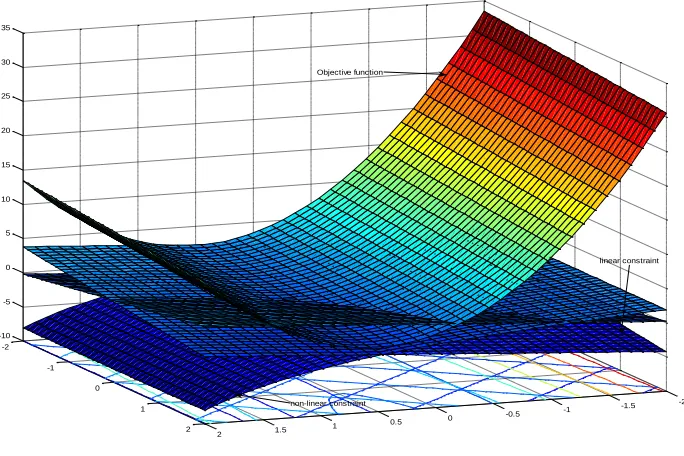
3.4 Feasible region and objective function in process synthesis problem. 59

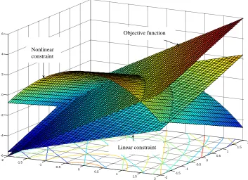
3.5 Objective function contours and nonlinear feasible region 61

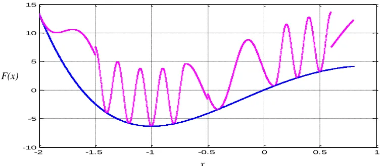
3.6 Objective function and augmented objective function 68

3.7 Behaviours of F(x) for the various penalty parameters S 68

3.8 Behaviours of F(x) for different discrete requirements. 69

3.9 Convergence Characteristics plots. 74

3.10 Convergence plot. 75

4.1 Flowchart of the proposed HCP algorithm. 89

4.2 Evolution plot for Himmelblau’s Function. 92

4.3 Tension/compression string design problem. 93

4.4 Performance of the minimisation of the weight of a tension spring problem. 94

4.5 Pressure vessel design problem. 95

4.6 Evolution plot of pressure vessel design. 96

4.7 Welded beam design problem. 97

4.8 Evolution plot of welded beam design problem. 98

4.9 The 10-Bar Planar Truss Structure. 99

4.10 Search process comparison for Himmelblau’s function. 102

5.1 Iteration procedure of Alternating Optimisation. 109

5.2 Objective function evaluations during the AO process. 119

6.1 The TVIW-PSO algorithm. 128

9

6.3 Branch-and-Bound tree. 134

6.4 Flowchart of the proposed HPB algorithm. 138

6.5 Performance comparison for the pressure vessel design problem. 142

6.6 Compression coil spring. 144

6.7 Performance comparison for the spring design problem. 145

6.8 Evolution plots of welded beam design. 147

6.9 Speed reducer design. 149

6.10 Evolution plots of speed reducer design. 150

10

List of abbreviations

 AO Alternating Optimisation.

 BB Branch and Bound.

 COP Constrained Optimisation Programming.

 DE Differential Evolution.

 DF Derivative-Free.

 DP Deterministic Programming.

 EA Evolutionary Algorithms.

 ECP Extended Cutting Plane.

 EP Evolutionary Programming.

 GBD Generalized Bender’s Decomposition.

 GO Global Optimisation.

 IP Integer Programming.

 GA Genetic Algorithms.

 LP Linear Programming.

 MDNLP Mixed Discrete Non-Linear Programming.

 MILP Mixed Integer Linear Programming.

 MINLP Mixed Integer Non-Linear Programming.

 MIP Mixed Integer Programming.

 MOO Multi-Objective Optimisation.

 MIQP Mixed Integer Quadratic Programming.

 NLP Non-linear Programming.

 OA Outer Approximation.

 PSO Particle Swarm Optimisation.

 QN Quasi-Newton.

 QP Quadratic Programming.

 SLP Successive Linear Programming.

 SP Stochastic Programming.

11

Notation

The set of real numbers.

Ν The set of non-negative integers.

Ø The empty set (without any element).

The set consisting of the three elements and .

is an element of the set .

is not an element of the set .

The number of elements in the set , the cardinality of .

The set of elements such that …

There exists an element such that …

For any element of .

Cartesian product of and .

A closed interval: , where a and b are real numbers (a ≤ b).

X x

x

 )

inf( If has a lower bound, then

X x

x

 )

inf( is by definition the largest of the lower bound

of .

If has no lower bound, then by convention inf(x).

 

x k x }

{ Sequence of elements , for

Cartesian product of the set , multiplied n times by itself.

The vector of with components

,

Transpose of the vector of .

Scalar product of the vector and .

Euclidian norm of the vector .

n j

m i ij a A

, , 1 , , 1 ] [

 

 



Matrix with m rows and n columns, is the element in row i and column j.

12

Rank(A) rank of matrix A ( dimension of the largest regular square submatrix of A).

If is a function of the variables

of f at the point x, that is the n-vector with components

Equivalent notation to mean , the transposed vector of

is thus the same as the row-matrix with components ,

.

If is a function of the variables

Hessian of f at the point x, that is the real (symmetrical) matrix whose

element is .

Subdifferential of f at x: set of the subgradients of f at x( for the convex or a

concave function).

)} ( {

inf f x

X

x By definition, infxX{f(x)}infxX(y) .

where and , y=f(x)}.

)} ( {

sup f x

X x

By definition sup{f(x)} inf{ f(x)}

X x X

x

  

 

)} (

{f x

Min X

x Let and . If xinfX{f(x)} and there exists xXsuch

that f(x) inf{f(x)}

X x

 ,then Min{f(x)} f(x)

X

x  . If  

)} ( {

inf f x

X

x , then by

convention  

 {f(x)} f(x)

Min X

x . If , then by convention

  

 {f(x)} f(x)

Min X

x .

)} (

{f x

Max X

x By definition: MaxxX{f(x)}MinxX{f(x)}.





13

Chapter 1

General Introduction

1.1 Overview

Optimisation problems are generally composed of three parts: an objective function that needs to be

optimised, a set of variables that define the problem and on which the objective function depends, and a

set of constraints that restrict feasible values of these variables. Constraints reduce the feasible space

wherein solutions to the problem can be found. Formulation of an optimisation problem involves taking

statements, defining general goals and requirements of a given activity, and transcribing them into a series

of well-defined mathematical statements. More precisely, the formulation of an optimisation problem

involves: selecting one or more optimisation variables, choosing an objective function, and identifying a

set of constraints. Optimisation algorithms need to ensure that a feasible solution is found. That is, the

optimisation algorithm should find a solution that both optimises the objective function and satisfies all

constraints. If it is not possible to satisfy all constraints, the algorithm has to balance the trade-off

between optimal objective function value and number of constrains violated.

Optimisation can be applied to all disciplines. Many recent problems in Engineering, Science, and

Economics can be presented as computing globally optimal solutions. Using classical nonlinear

programming techniques may fail to solve such problems because these problems usually contain

multiple local optima [1]. Therefore, global search methods should be invoked in order to deal with such

14

1.2 Objectives

In this research, constrained optimisation problem is considered in the continuous and discrete search

space. The overall objectives of the present thesis were to develop novel hybrid versions of hybrid

evolutionary approaches as promising solvers for the considered problems. The designed algorithms

aimed to overcome the drawbacks of slow convergence and random constructions of stochastic methods.

In these hybrid methods, local search strategies are inlaid inside the evolutionary approaches in order to

guide them especially in the vicinity of local minima, and overcome their slow convergence especially in

the final stage of the search.

The optimisation problems exist in many applications and achieving the exact global solution is neither

possible nor desirable. Therefore, using efficient global search methods is highly needed in order to

achieve optimal global solutions. It has been found that evolutionary algorithms produce good results

when applied to these problems and they could obtain highly accurate solutions in many cases [2]. The

power of evolutionary techniques come from the fact that they are robust and can deal successfully with a

wide range of problem areas. However, these methods, especially when they are applied to complex

problems, suffer from the slow convergence and the high computational cost. The main reason for this

slow convergence is that these methods explore the global search space by creating random movements

without using much local information about promising search direction. In contrast, local search methods

have faster convergence due to their using local information to determine the most promising search

direction by creating logical movements. However, local search methods can easily be entrapped in local

minima.

Our work has the objective to combine evolutionary approaches with gradient-based search methods to

design more efficient algorithms with relatively faster convergence than the pure evolutionary methods.

Furthermore, these hybrid methods are not easily entrapped in local minima because they still maintain

15

are developed in order to deal with the global optimisation problems that have the above characteristics.

Specifically, local search guidance in the direct search methods is invoked to direct and control the global

search features of evolutionary approach to design more efficient hybrid methods.

1.3 Organisation and Contributions

In this thesis, details of the implementation are rather technical, thus it makes sense to firstly investigate

the details of the optimisation approaches for solving constrained optimisation problems, and demonstrate

some examples of the implemented algorithms. Secondly, theoretical and technical details of the

developed methods appear towards the end of the thesis detailing the lower level aspects of our

approaches.

The thesis is organised into seven chapters as follows:

 The first chapter is introduction to this research program in which novel and generic optimisation

methods were developed and implemented in order to tackle constrained optimisation problems.

 In chapter 2, some well-known deterministic and stochastic search methods are introduced to be

used throughout this study. Stochastic search methods are a relatively recent development in the

optimisation field, aimed to tackle difficult problems, such as ones afflicted by

non-differentiability. Although a casual understanding of some deterministic methods will be useful

here, especially where the methods are analogous to certain stochastic approaches.

 The third chapter presents the solution of a collection of test models for continuous and

mixed-variables nonlinear programming. It also introduces some modern solvers that are used for

solving such problems. Results are reported for testing a number of existing state-of-the-art

solvers for global constrained optimisation and constraint satisfaction on different test problems,

collected from the literature. This chapter also shows the implementation of different

16

 In chapter 4, a new hybrid coevolutionary algorithm is presented. This approach is capable of

solving difficult real-world constrained optimisation problems formulated as min-max problems

with the saddle point solution. A two-group model has been considered; in such models

individuals from the first group interact with individuals from the second through a common

fitness evaluation based on payoff matrix game. The new approach is fast and capable of global

search because of combining particle swarm optimisation and gradient search to balance

exploration and exploitation. When applying this algorithm to specific real-world problems, it is

often found that the addition of gradient-search mechanism can aid in finding a good global

optimal solution. The developed algorithm is particularly suited for difficult optimisation

problems in the sense that the objective function and the constraints are nonsmooth functions and

the problem has multiple local extrema.

 The fifth chapter introduces an original method for solving general Mixed Discrete Non-Linear

Programming problems, based on the generic framework of Alternating Optimisation and

Augmented Lagrangian Multipliers method. An iterative solution strategy is proposed by

transforming the constrained problem into two unconstrained components or units; one solving

for the discrete variables, and another for the continuous ones. During the search process, each

unit focuses on minimising a different set of variables while the other type is frozen. While

optimising each unit, the penalty parameters and multipliers are consecutively updated until the

solution moves towards the feasible region. The performance of the algorithm is evaluated against

real-world benchmark problems; the experiment results indicate that the algorithm achieves an

exact global solution with better computational cost compared to the existing algorithms.

 The sixth chapter, we developed a hybrid particle swarm optimisation with branch and bound

architecture, which is based on the fact that the evolutionary algorithm has the ability to escape

from local minima, while the gradient-based method exhibits faster convergence rate. The

17

the same time mitigates significantly their aforementioned weaknesses. It is particularly suited for

difficult nonlinear mixed discrete optimisation problems, in the sense that the objective function

and the constraints are non-smooth functions and have multiple local extrema. The algorithm

takes advantage of the rapid search of BB, when the evolutionary method has discovered a better

solution in its globally processed search space. The hybridisation phase of the new algorithm

depends primarily on a selective temporary switching from particle swarm optimisation and

branch and bound methods, when it appears that the current optimum can be potentially

improved. As will be described later, any such potential improvement is recorded and

broadcasted to the entire swarm of the particles via its social component update. The validity,

robustness and effectiveness of the proposed algorithm are exemplified through some well known

benchmark mixed discrete optimisation problems

 The seventh chapter presents Conclusions and issues for further work, and indicate the potential

usefulness of the developed approaches.

It has been found that applying a complete local search method in the final stage of the evolutionary

search techniques helps them to obtain good accuracy quickly. The new hybrid methods are promising in

practice and competitive with the other compared methods in terms of computational costs and the

success of obtaining the global solutions. The algorithm developed in chapter 4 shows a superior

performance in terms of the solution qualities against the compared methods. In Chapter 5 and 6, two new

algorithms have been proposed as hybrid methods that combine specific strategies to fit the the

development of the field of general mixed discrete nonlinear programming. Inheriting the advantages of

the deterministic and stochastic approaches, the new methods are efficient and capable of global search.

Simulation results based on well-known mixed continuous-discrete engineering design problems

demonstrate the effectiveness and robustness of the proposed algorithm. The deterministic search method

scheme applied in the final stage can overcome the slowness of the evolutionary algorithm in its final

18

in practice and competitive with some other population-based methods in terms of the solution qualities.

The numerical results shown in chapters 3–6 show that creating gradient-based techniques while applying

stochastic approach in the proposed methods give better performance of metaheuristics. In addition,

accelerating the final stage of the evolutionary methods by applying a complete local search technique

19

Chapter 2

Methods for Constrained Optimisation

2.1 Introduction

This Chapter introduces the reader to elementary concepts of generic formulations for linear and

nonlinear optimisation models, and provide some illustration for different optimisation methods. In

general, there are two classes of optimisation methods for solving continuous and mixed discrete design

problems: stochastic and deterministic ones. Stochastic search methods are a relatively recent

development in the optimisation field, aimed to tackle difficult problems, such as ones afflicted by

non-differentiability, multiple objectives and lack of smoothness. Although a casual understanding of some

deterministic methods will be useful here, especially where the methods are analogous to certain

stochastic approaches. In this chapter, some well-known deterministic methods and metaheuristics are

introduced to be used throughout this study.

2.2 Deterministic Search Techniques

This section has its objective the discussion of techniques, most of which are derived from the

gradient-based algorithms literature. It deals with techniques that are applicable to the solution of the continuous

20

 

 

 

n j

i x

X x

,l , j , x h

,m , i , x g s.t

x f Min

  

 

 





 

 

1 0

1 0

(2.1)

where x represents a vector of n real variables subject to a set of m inequality constraints g(x) and a

set of l _{equality constraints} h(x).

There are many techniques available for the solution of a constrained nonlinear programming problem.

All the methods can be classified into two broad categories: direct methods and indirect methods. In the

direct methods, the constraints are handled in an explicit manner, whereas in most of the indirect

methods, the constrained problem is solved as a sequence of unconstrained optimisation problems [3].

In this section, direct search methods are presented in order to deal with the constrained optimisation

problems that have the above characteristics. In this research, local search guidance in the direct search

methods is invoked to direct and control the global search features of metaheuristics to design more

efficient hybrid methods. In the rest of this chapter, some well-known direct and indirect search methods

are introduced briefly to be used throughout this study. These techniques can be classified as follows:

 Direct Search Methods

 Random search methods.

 Heuristic search methods.

 Complex methods.

 Objective and constraints approximation methods.

 Sequential quadratic programming method.

 Methods of feasible directions.

 Zoutendijk’s method.

 Rosen’s gradient projection method.

21

 Indirect Search Methods

 Transformation of variables techniques.

 Sequential unconstrained optimisation techniques.

 Interior penalty function method.

 Exterior penalty function method.

 Augmented Lagrange multiplier method.

These search methods have been designed for solving unconstrained optimisation problems. However,

constrained handling techniques can be used to deal with constrained optimisation problems. More details

about these methods can be found in [4].

2.2.1 Mixed Integer Continuous Programming

Mixed Integer Programming (MIP) refers to mathematical programming with continuous and discrete

variables and linearity or non-linearity in the objective function and constraints. The use of MIP is a

natural approach of formulating problems where it is necessary to simultaneously optimise the system

structure (discrete) and parameters (continuous). These problems arise when some of the variables are

required to take integer values. MIPs have been used in various applications, including the process

industry and the financial, engineering, management science and operations research sectors.

A mixed-integer linear program (MILP) is a mathematical program with linear constraints in which

specified subsets of the variables are required to take on integer values. Although MILPs are difficult to

solve in general, the past ten years has seen a dramatic increase in the quantity and quality of software -

both commercial and non-commercial - designed to solve MILPs. The MILP formulation with 0-1

22 Q

n T

{0,1} y

X x , 0 x

subject to

C min



   

 

 b By Ax

y d

x T

(2.2)

where, x is a vector of n continuous variables,

y is a vector of q 0-1 variables,

,c d are n1 and q1 vectors of parameters, ,A B are matrices of appropriate dimension, b is a vector of p inequalities.

Mixed Integer Linear programming methods and codes have been available and applied to many practical

problems for more than twenty years. The major difficulty that arises in mixed- integer linear

programming MILP problems for the form (2.2) is due to the combinatorial nature of the domain of y

variables. Any choice of 0 or 1 for the elements of the vector y results in a LP problem on the x variables

which can be solved for its best solution.

One may follow the brute-force approach of enumerating fully all possible combinations of 0 -1 variables

for the elements of the y vector. Unfortunately, such an approach grows exponentially in time with

respect to its computational effort. For instance, if we consider one hundred 0 -1 y variables then we

would have 2100 possible combinations. As a result, we would have to solve 2100 LP problems. Hence,

such an approach that involves complete enumeration becomes prohibitive [1]. MINLP refers to

mathematical programming with continuous and discrete variables and nonlinearities in the objective

function and constraints. MINLP problems are difficult to solve, because they combine all the difficulties

of both, the nature of mixed integer programs (MIP) and the difficulty in solving convex or nonconvex

23

MINLPs have been used in various applications, including the process industry and the financial,

engineering, management science and operational research sectors. As the number of binary variables y

in form (2.2) increase, one is faced with a large combinatorial problem, and the complexity analysis

results characterize the MINLP problems as NP- complete. At the same time, due to the nonlinearities the

MINLP problems are in general nonconvex which implies the potential existence of multiple local

solutions.

Considerable interest was shown for discrete variables engineering optimisation problems in the late

1960s and early 1970s. However, at that time optimisation methods for continuous nonlinear

programming (NLP) problems were not developed, so the focus shifted to the development and evolution

of numerical algorithms for such problems. In the 1970s and 80s, substantial effort was put into

developing and evaluating algorithms for continuous NLP problems. Therefore, in recent years, the focus

has shifted back to applications of optimisation techniques to practical engineering problems that

naturally used mixed discrete and continuous variables in their formulation [4] .The component structure

of MIP and NLP within MINLP provides a collection of natural algorithmic approaches. They can be

classified as:

 Classical solution methods

 Branch and Bound (BB)

 Outer Approximation (OA)

 Extended Cutting Plane methods (ECP)

 Generalized Bender’s Decomposition (GBD)

 Hybrid methods

 LP/NLP based Branch and Bound

 Integrating SQP with Branch-and-Bound

 Sequential Cutting Plane (SCP)

24

In the rest of this chapter, the important details of these methods are explained to be used throughout this

study. Implementation and numerical examples will be presented in the following chapters.

2.2.2

Branch and Bound method

A general branch and bound method for MIP problems is based on the key ideas of separation, relaxation,

and fathoming [2]. The branch and bound (BB) method starts by solving first the continuous NLP

relaxation. If all discrete variables take integer values the search is stopped. Otherwise, a tree search is

performed in the space of the integer variables. Then the algorithm selects one of those integer variables

which take a non-integer value, and branch on it.

Branching generates two new sub problems by adding simple bounds to the NLP relaxation. One of the

two new NLP problems is selected and solved next. If the integer variables take non-integer values then

branching is repeated. If one of the fathoming rules is satisfied, then no branching is required, and the

corresponding node has been fully explored. The fathoming rules are:

- Infeasible solution is detected.

- An integer feasible node is detected.

- A lower bound on the NLP solution of a node is greater or equal than the current upper bound.

Once a node has been fathomed the algorithm backtracks to another node which has not been fathomed

until all nodes are fathomed.

Branching variable selection

Since branching is in the core of any BB algorithm, finding good strategies was important to practical

MIP solving right from the beginning. Suppose we have chosen an active node

i

non-linear programming solution

x

25

1. Lowest-Index-First:

It is possible to have some information on the importance of some of the integer variables in a given

model. The integer variables are arranged in order of importance, the most important of these being

processed first. This is accomplished by indexing the variables with the decreasing priorities of the

integer variables and selecting the variable with the lowest index first.

2. Most Fractional Integer variables:

This strategy selects the variable which is farthest from the nearest integer value. This choice is aimed at

getting the largest degradation of the objective when branching is carried out so that more nodes can be

fathomed at an early stage.

3. Use of Pseudo-Costs:

The concept of Pseudo-cost was first developed for solving mixed integer linear programming problems.

The pseudo-costs are used as a quantitative measure of the importance of the integer variables and this

allows the assignment of some priority to the variables. For each integer variablex_jtwo quantities are

defined, lower pseudo-cost (pcl_j) and upper pseudo-cost (pcu_j). The values of the lower and upper

pseudo-costs are computed during the tree search.

Selection of Branching Node

The selection method for branching node may significantly affect the performance of branch and bound

algorithm [1]. The most commonly used branching strategies are:

 Depth-first:

Whenever a branching is carried out the nodes corresponding to the new problems are given

preference over the rest of the unfathomed nodes. The child nodes are created as the next nodes to

optimise.

 Best-first:

In this strategy, the node which currently has the lowest bound in the objective is selected for

26

 Breadth-first:

We examine a certain level in the tree entirely before proceeding to the next level in the tree in order

to get shorter search paths in the tree.

Hybrid methods

 Depth-first-then-breadth:

In the method a depth first search is performed until the first solution is found. The algorithm then

switches to a breadth first search strategy.

 Depth-first-then-best:

As the previous method, a depth first strategy is performed until the first solution is found, then

switching to a best first method.

 Depth-first-with-backtracking:

Backtracking is a systematic way to go through all the possible configurations of a space.

2.2.3

Outer Approximation method

This algorithm is based on the concept of defining an MILP master problem. Relaxations of such a master

problem are then used in constructing algorithms for solving the MINLP problem. The method presented

here is a generalization of Outer approximation proposed by Duran and Grossman [5]. We shall next

present the reformulation of P as an MILP master problem. Based on this reformulation an algorithm is

presented which solves a finite sequence of NLP sub problems and a MILP or MIQP master problem,

respectively.

The MINLP model problem P is reformulated as an MINLP problem using Outer approximation; the

reformulation employs projection onto the integer variables and linearization of the resulting NLP sub

problems by means of supporting hyper planes.

It can be shown that it suffices to add the linearisation of strongly active constraints to the master

27

solved in the Outer Approximation Algorithms. In this subsection the simplifying assumption is made that

all are feasible. The first step in reformulating P is to define the NLP sub problem.

min ( , )

( )

. . ( , ) 0 j

x j

j

x X

f x y NLP y

s t g x y



 

 _

 (2.3)

In which integer variables are fixed at the value yyj. By definingv y( j)as the optimal value of the sub

problemNLP y( j)it is possible to express P in terms of a projection onto the y variables, that is

min( ( ))

j

j

y Y

v y



    



   



integer ) ( ) ( subject to

minimise

problem Master

,

Y y

Y y y y

f_{i i} T _{j j}

y

 

 

(2.4)

The assumption that all are feasible implies that all sub problems are feasible. Letxjdenote an optimal

solution of NLP(yj) for yjY. In order to derive a correct representation it is necessary to consider how

NLP solvers detect infeasibility. Infeasibility is detected when convergence to an optimal solution of a

feasibility problem occurs. At such an optimum, some of the nonlinear constraints will be violated and

other will be satisfied and the norm of the infeasible constraints can only be reduced by making some

feasible constraints infeasible. The equivalent MILP problem is

, ,

j j T

j T

j min

. + [ ]

0 [ ]

y Y , x X , y Y integer

x y

j j j j

j

x x

s t f f

y y

MILP

x x

g g

y y

 



 

 

    

 

 _ _ 



 _{ } 

  

 

  

    

 _{ } 



 

 

 _{   } 

 

(2.5)

The relaxation of the master problem can be employed to solve the model problem P. The resulting

algorithm is shown to iterate finitely between NLP sub problems and MILP master problem relaxations.

28

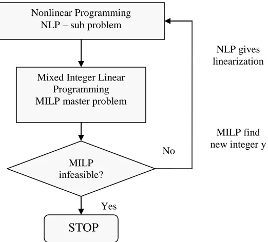
Linear Outer Approximation Algorithm:

- Initialisation

Repeat i0,T1,S1,UBD1

Where T 









S 

1. Solve NLP(y_j) of F(y_j),the solution is x_j

2. Linearize Objective and constraints function about (xj,yj).

3. If (NLP(yj) feasible ) Then

update current best point by setting x*xj,y*y UBDj, fi

else UBDjUBDj1

4. Solve the current relaxation Mj of the master program M, giving a new .

5. Set j = j+1 Until (Mj is infeasible).

Fig. 1.1 Linear Outer Approximation algorithm. Nonlinear Programming

NLP – sub problem

Mixed Integer Linear Programming MILP master problem

MILP infeasible?

No

Yes

MILP find new integer y

NLP gives linearization

29

2.2.4

Extended Cutting Plane method

The ECP method, which is an extension of Kelly’s cutting plane algorithm for convex NLP, does not rely

on the use of NLP sub problems and algorithms [2]. It relies only on the iterative solution of the problem

(M-MIP) by successively adding a linearization of the most violated constraint at the predicted point

^ k

j

( k, k) : k { arg {max g ( k,y ) }

j J

x y J J x



  (2.6)

Convergence is achieved when the maximum constraint violation lies within the specified tolerance. The

optimal objective value of (M-MIP) yields a non-decreasing sequence of lower bounds. It is possible to

either add to (M-MIP) linearization of all the violated constraints in the setJk, or linearization of all the

nonlinear constraints jJ. In the ECP method the objective must be defined as a linear function, which

can easily be accomplished by introducing a new variable to transfer nonlinearities in the objective as an

inequality.

The ECP method is able to solve MINLP problems, including general integer variables and not only

binary variables, and no integer cuts are needed to ensure convergence. ECP methods are oftenly claimed

to have slow convergence. The number of non-linear function evaluations used to obtain the optimal

solution has in several cases been even magnitudes lower than when using MINLP methods based on

solving NLP sub problems.

2.2.5

Generalized Bender’s Decomposition (GBD) method

The GBD method is similar to the Outer- Approximation method [1]. The difference arises in the

definition of the MILP master problem (M-MIP). The first step is to express P in terms of a projection

onto the integer variables





 

 ( )

min

Proj(P) '

yj

j

V v y (2.7)

30

The optimal value of the NLP sub problems defined by:

 

 

      

 

 

) ( ,

0 ,

subject to , minimise

NLP ,

Y converged y

X x

y y

y x g

y x f

j y

x

(2.8)

Benders’ Decomposition is able to treat certain nonconvex problems that are not readily solved by other

methods such as BB or OA.

The reformulation does not contain the continuous variables x:

    



   



integer

) ( ) ( subject to

minimise

problem Master

,

GBD

Y y

Y y y y

f_{i i} T _{j j}

y

 

 

(2.9)

Decomposition models with integer variables usually decompose into a master problem that comprises al

the integer variables and sub problems, which evaluate the remaining variables. Sub problems with

integer variables introduce additional difficulties and require the use of nonlinear duality theory.

2.2.6 LP/NLP based Branch and Bound

This approach covers problems with nonlinearities in the integer variables. The motivation for the

LP/NLP based branch and bound algorithm is that outer approximation usually spends an increasing

amount of computing time in solving successive MILP master problem relaxation. This approach avoids

the re-solution of MILP master problem relaxation by updating the branch and bound tree. Instead of

solving successive relaxations of M, the algorithm solves only one MILP problem which is updated as

new integer assignments are encountered during the tree search [2].

Initially an NLP sub problem is solved and the initial master program relaxation is set up from the

supporting hyperplanes at the solution of the NLP - sub problem. The MILP problem is then solved by a

31

Algorithm

1. Consider MILP branch and bound.

2. Interrupt MILP, when yj found.

3. Solve NLP (y_j) to get x_j.

4. Linearisef ,c about (xj,yj)

5. Add linearization to tree.

6. Continue MILP tree search.

Until

lower bound > upper bound

As in the two outer approximation algorithms the use of an upper bound implies that no integer

assignment is generated twice during the tree search. Since both the tree and the set of integer variables

are finite the algorithm eventually encounters only infeasible problems and the stack is thus emptied so

that the procedure stops.

This method can also be applied to the GBD and ECP methods. The LP/NLP method commonly reduces

quite significantly the number of nodes to be enumerated. The trade-off is that the number of MLP sub

problems may increase. This method is better suited for problems in which the bottleneck corresponds to

the solution of the MILP master problem.

2.2.7

Integrating SQP with Branch-and-Bound

An alternative to nonlinear branch-and-bound for convex MINLP problems is due Borchers and Mitchell

[6]. They observed that it not necessary to solve the NLP at each node to optimality before branching and

propose d an early branching rule, which branches on an integer variable before the NLP has converged.

The algorithm is based on branch and bound, but instead of solving an NLP problem at each node of the

tree, the tree search and the iterative solution of the NLP are interlaced. Thus the nonlinear part of (P) is

solved whilst searching the tree. The nonlinear solver that is considered in this method is a Sequential

Quadratic Programming (SQP) solver. The basic idea underlying this approach is to branch early –

32

This approach has a similar motivation as the Outer Approximation algorithm [5] but avoids the

resolution of related MILP master problems by interrupting the MILP branch and bound solver each time

an integer node is encountered. At this node an NLP problem is solved and new outer approximations are

added to all problems on the MILP branch and bound tree. Thus the MILP is updated and the tree search

resumes.

Algorithm

1. Initialisation: Obtain the continuous relaxation of P

2. Set the upper bound to infinity

3. While (there are pending nodes in the tree) do

 Select an unexplored node

 Repeat (SQP iteration)

Solve QPs for a step dk.

if (QPs infeasible) then fathom node and exit

Set ₍ k 1_, k 1_{) (} k_, k_{) (} k_, k₎

x y

x  y   x y  d d

if( (y(k1)) integral ) then

Update current best point by setting

( ,x y* *)(xk1,yk1),f* fk1 and U f*

else choose a non integral y(k1) and branch

endif

exit

endif

4. Compute the integrity gap  max |_i y_ik1round y( _ik1) |

5. if (

 

- Choose a non-integral y(k1)and branch, exit

end if

end while

The value of is suggested for the early branching rule and this value has also been chosen here.

The algorithm has to be modified if a line search or a trust region is used to enforce global convergence

33

by branching is equivalent to the parent problem. This algorithm has two important advantages. First, the

lower bounding can be implemented at no additional cost. Secondly, the lower bounding is available at all

nodes of the branch and bound tree.

2.2.8

Sequential Cutting Plane (SCP)

This algorithm integrates cutting plane techniques with branching techniques. Rather than solving a

linearized MILP problem to feasibility or optimality, it applies cutting planes in each node of the branch

and bound tree. The technique differs from the-ECP method, where the generation of cutting planes is

separated from the branching process [7]. For the NLP sub problems, we solve a sequence of linear

programming (LP) problems. Note that the SCP algorithm could also be considered to be a form of

Successive Linear Programming (SLP). However, a more general version of the SCP algorithm could, if

desired, also retain the cutting planes between the LP sub iterations. The algorithm also generates explicit

lower bounds for each node in the branch and bound tree. The algorithm obtains explicit lower bounds on

the nodes when performing NLP iterations in the nodes.

The first LP sub iteration within NLP iteration provides a lower bound on the node. When branching, the

child nodes inherit the lower bound of the parent node. Whenever the current upper bound is improved,

you may drop any node with a lower bound greater than or equal to the current upper bound. You may,

therefore, in some cases drop nodes in the tree without solving any additional LP problems for those

nodes. Explicit lower bounds have a significant impact on the convergence speed as it means less sub

problems solved.

The algorithm builds a branch and bound tree where each node represents a relaxed NLP sub problem of

the original problem (P). Each NLP sub problem is solved using a sequence of LP problems, but the NLP

sub problem is not solved to optimality. We then choose an integer variable with a non-integral value in

34

problem in an NLP iteration provides a lower bound for the optimal value of the NLP sub problem. The

lower bounds of the nodes can be used for removing nodes from the tree any time we improve the

currently best known solution for the original problem (P).

The algorithm does not solve the NLP sub problems to optimality. It interrupts the NLP procedure before

an optimal point has been found in order to make the branch and bound algorithm faster. If the current

iteration is converging to a non-integral point, we may branch early on any variable in yk that has a

non-integral value, rather than waste effort on finding an optimal, non-integer, solution for the current sub

problem.

The algorithm uses an NLP version of the Sequential Cutting plane algorithm to solve the NLP sub

problems. The difference from the SQP approach is that it solves a sequence of LP problems rather than

QP problems in order to find a solution to the NLP sub problems.

2.2.9

Outer-Approximation based Branch-and-Cut algorithm

The algorithm integrates Branch and Bound, Outer Approximation and Gomory Cutting Planes [5]. Only

the initial Mixed Integer Linear Programming (MILP) master problem is considered. At integer solutions

nonlinear Programming (NLP) problems are solved, using a primal-dual interior point algorithm. The

objective function and constraints are linearised at the optimum solution of those NLP problems and the

linearisations are added to all the unsolved nodes of the enumerations tree. Also, Gomory cutting planes,

which are valid throughout the tree, are generated at selected nodes. These cuts help the algorithm to

locate integer solutions quickly and consequently improve the linear approximation of the objective and

constraints, held at the unsolved nodes of the tree.

The complete algorithm is described in the following:

Algorithm

1. Initialisation:  _o {0,1}p is given; set    1 

^ 1 ^ ,

1T S

i .

35

2.1 If NLP(



^

0 {0}

T  .

Otherwise solveF(



^

0 {0}

S  . Let

x





2.2 If

x



UBD



f x

( ,



)

Otherwise set

UBD

 

2.3 Linearise objective and constraints about

( ,

x



)

^ 0

M .

2.4 Define ^

0

M as the root of the search tree. Let be the list which contains the unsolved nodes and set.

3. Node selection: If  



i i

R R and remove it from the list.

4. Solve the LP relaxation of the 0-1 MILP problem ^

i

M and let

^ ^

( , , )x  be its optimum solution.

5. If ^

{0,1}p

 then

5.1 Set ^ i

  and solve NLP(i) if it is feasible or F(i) otherwise. Let

x

or F(_i).

5.2 Linearise objective and constraints around (

x

^ ^

1 { }

i i

T T_  i or

^ ^

1 { }

i i

S S_  i as

appropriate.

5.3 Add the linearisations to ^

i

M and to all the nodes in. Place

^ i

M back in.

5.4 Update incumbent solution and upper bound:

If NLP(_i) is feasible and ( ,f x_i_i) <

UBD

( ,

x



) ( ,



x



)

UBD



UBD

5.5 Pruning: Delete all nodes fromwith





UBD

Go to Step 3

6. If ^

{0,1}p

 then

6.1 Cutting versus Branching Decision: If cutting planes should be generated then go to Step 6.2.

Otherwise go to Step 6.3

6.2 Cut generation: Generate a round of Gomory mixed integer cuts using every row corresponding to a

36

Add all those cuts to ^

i

M and store them in the pool. Go to step 4.

6.3 Branching: Select a violated 0-1 variable in ^

 say (0,1)

) ( ^

 r

 . Create two new nodes

1 1

0 1 0 1

(Ri,Ri)(Ri { },r Ri) and (R₀i1,R₁i1)(R R₀i, ₁i{ })r .

Add both nodes to the list. Go to Step 4.

If

UBD

 

( ,

x



)

0-1 MINLP problem. Otherwise the problem is infeasible.

Algorithm OA-BC requires an initial 0-1 vector to be given by the user. If such a vector is not available

then the algorithm can start by solving the NLP relaxation of the initial 0-1 MINLP problem. If the

solution of the NLP relaxation satisfies all the integrality constraints then that solution also solves the

initial 0-1 MINLP problem and the algorithm can stop. If the NLP relaxation is infeasible then the initial

0-1 MINLP problem is also infeasible and the algorithm can stop. Finally if the NLP relaxation is feasible

and has a non-integer optimum solution, then the initial 0-1 MILP master problem can be formulated by

37

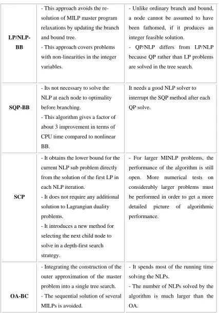
2.3 Comparison of MINLP optimisation methods

The MINLP optimisation methods represent quite different solution approaches. A comparison between

all these methods can be described as the following:

Comparison of MINLP methods

Method Advantages Disadvantages

BB

Finds an optimal solution if the

problem if of limited size and

enumeration can be done in

reasonable time.

Extremely time consuming. The

number of nodes in a branching tree

can be too large.

OA

Avoids solving huge number of

nonlinear programming problems.

- Potentially large number of

iterations.

- Adding Hessian term to the MILP

becomes MIQP.

ECP

- Only solving MILP problems

instead of NLP problems, in each

iteration the nonlinear constraints

need not be calculated at relaxed

values of the integer variables.

- solves MINLP problems

including general integer variables

and not only binary variables.

- It has slow convergence.

- The most time consuming step in

the ECP algorithm is the solution of

the MILP sub problems.

GBD

- Solves a large scale of linear

programs.

- Problems have a special structure

called Block Diagonal structure.

- Only active inequalities are

considered.

The MILP master problem is given

by a dual representation of a

38

LP/NLP-BB

- This approach avoids the re-

solution of MILP master program

relaxations by updating the branch

and bound tree.

- This approach covers problems

with non-linearities in the integer

variables.

- Unlike ordinary branch and bound,

a node cannot be assumed to have

been fathomed, if it produces an

integer feasible solution.

- QP/NLP differs from LP/NLP

because QP rather than LP problems

are solved in the tree search.

SQP-BB

- Its not necessary to solve the

NLP at each node to optimality

before branching.

- This algorithm gives a factor of

about 3 improvement in terms of

CPU time compared to nonlinear

BB.

It needs a good NLP solver to

interrupt the SQP method after each

QP solve.

SCP

- It obtains the lower bound for the

current NLP sub problem directly

from the solution of the first LP in

each NLP iteration.

- It does not require any additional

solution to Lagrangian duality

problems.

- It introduces a new method for

selecting the next child node to

solve in a depth-first search

strategy.

- For larger MINLP problems, the

performance of the algorithm is still

open. More numerical tests on

considerably larger problems must

be performed in order to get a more

detailed picture of algorithmic

performance.

OA-BC

- Integrating the construction of the

outer approximation of the master

problem into a single tree search.

- The sequential solution of several

MILPs is avoided.

- It spends most of the running time

solving the NLPs.

- The number of NLPs solved by the

algorithm is much larger than the

OA.

39

2.4 Evolutionary Programming

A large number of Evolutionary Algorithms (EA) have been developed. These EAs can be grouped based

on how individuals are represented, which evolutionary operators are used, and how these are

implemented. This chapter discusses briefly the concepts of Evolutionary and Coevolutionary

Programming. Evolutionary Algorithms can be classified into two classes; population-based methods and

point-to-point methods. In the latter methods, the search invokes only one solution at the end of each

iteration from which the search will start in the next iteration. The population-based methods invoke a set

of many solutions at the end of each iteration. This chapter highlights the principles of genetic algorithms,

particle swarm optimisation, and differential evolution as examples of population-based methods, and

simulated annealing as an example of point-to-point methods.

2.4.1 Simulated Annealing

Simulated annealing is a simple technique that can be used to find a global optimiser for continuous,

integer and discrete nonlinear programming problems. The approach does not require continuity or

differentiability of the problem functions because it does not use any gradient or Hessian information [8].

The SA algorithm successively generates a trial point in a neighbourhood of the current solution and

determines whether or not the current solution is replaced by the trial point based on a probability

depending on the difference between their function values. Convergence to an optimal solution can

theoretically be guaranteed only after an infinite number of iterations controlled by a procedure called

cooling schedule. The main control parameter in the cooling schedule is the temperature parameter T. The

main role of T is to let the probability of accepting a new move be close to 1 in the earlier stages of the

search and to let it be almost zero in the final stage of the search. A proper cooling schedule is needed in

40

2.4.2 Genetic algorithms

A genetic algorithm (GA) is a procedure that tries to mimic the genetic evolution of a species.

Specifically, GA simulates the biological processes that allow the consecutive generations in a population

to adapt to their environment. The adaptation process is mainly applied through genetic inheritance from

parents to children and through survival of the fittest. Therefore, GA is a population-based search

methodology. Nowadays, GAs are considered to be the most widely known and applicable type of

metaheuristics [9].

GA starts with an initial population whose elements are called chromosomes. The chromosome consists

of a fixed number of variables which are called genes. In order to evaluate and rank chromosomes in a

population, a fitness function based on the objective function should be defined. Three operators must be

specified to construct the complete structure of the GA procedure; selection, crossover and mutation

operators. The selection operator cares with selecting an intermediate population from the current one in

order to be used by the other operators; crossover and mutation. In this selection process, chromosomes

with higher fitness function values have a greater chance to be chosen than those with lower fitness

function values. Pairs of parents in the intermediate population of the current generation are

probabilistically chosen to be mated in order to reproduce the offspring. In order to increase the

variability structure, the mutation operator is applied to alter one or more genes of a probabilistically

chosen chromosome. Finally, another type of selection mechanism is applied to copy the survival

members from the current generation to the next one. The GA operators of selection, crossover and

mutation have been extensively studied. Many effective settings of these operators have been proposed to

fit a wide variety of problems. The GA algorithm can be described as follows:

Algorithm



P