promoting access to White Rose research papers
White Rose Research Online
Universities of Leeds, Sheffield and York
http://eprints.whiterose.ac.uk/
This is an author produced version of a paper published in
Acta Materialia.
White Rose Research Online URL for this paper:
http://eprints.whiterose.ac.uk/4984/
Published paper
Rosam, J., Jimack, P.K. and Mullis, A.M. (2008)
An adaptive, fully implicit
multigrid phase-field model for the quantitative simulation of non-isothermal
binary alloy solidification.
Acta Materialia, 56 (17). pp. 4559-4569.
An Adaptive, Fully Implicit Multigrid Phase-Field Model for the Quantitative Simulation of
Non-isothermal Binary Alloy Solidification.
J. Rosam†§, P.K. Jimack§ & A.M. Mullis†*
Institute for Materials Research† & School of Computing§, University of Leeds, Leeds, LS2-9JT.
Abstract
Using state-of-the-art numerical techniques such as mesh adaptivity, implicit time-stepping and a non-linear multi-grid solver the phase-field equations for the non-isothermal solidification of a dilute binary alloy have been solved. Using the quantitative, thin-interface formulation of the problem we have found that at high Lewis number a minimum in the dendrite tip radius is predicted with increasing undercooling, as predicted by marginal stability theory. Over the dimensionless undercooling range 0.2 - 0.8 the radius selection parameter, σ*, was observed to vary by over a factor of two and in a non-monotonic fashion, despite the anisotropy strength being constant.
Introduction
One of the most fundamental and all pervasive microstructures produced during the solidification of metals is the dendrite. Remnants of these dendritic microstructures often survive subsequent processing operations, such as rolling and forging, and the length scales established by the dendrite can influence not only the final grain size but also micro- and hence macro-segregation patterns. This can have a wide-ranging influence on both the properties of finished metallic products, affecting for instance mechanical properties, corrosion resistance and surface finish, and on the formability of metallic feedstock, such as the ability to resist hot tearing during rolling.
Where dendritic growth has been observed directly, in transparent analogue casting systems such as succinonitrile[ ]1 and xenon[ ]2, the evidence is that the morphology of dendrites grown at different
undercoolings is probably self-similar when scaled against the tip radius, ρ. Consequently all the more obvious length scales of the dendrite are simple multiples of ρ, thus making the ability to predict ρ accurately a problem of central importance to the theory of dendritic growth.
The problem of predicting ρ first became apparent in 1947 when Ivantsov[ ]3 showed that an isothermal
paraboloid of revolution, growing at velocity V into an undercooled melt was a shape preserving solution to the diffusion equation, thus giving rise to the idea of the parabolic needle dendrite. The analytical solution for such a crystal growing into its undercooled melt is degenerate in that it relates the Peclet number, and not the growth velocity, to undercooling, where the Peclet number is defined as
α ρ 2 =V
Pt (1)
with α the thermal diffusivity in the melt. Consequently, at a given undercooling an infinite set of solutions are admissable, subject to the condition Vρ = constant. Such degeneracy is not observed in nature, where a well defined growth velocity can always be associated with a given undercooling, thus sparking the search for an additional mechanism to set the length scale, ρ, for the dendrite.
One of the most enduring solutions to this problem is based on a linear stability analysis of a plane solidification front against the growth of small perturbations[ ]4. This theory postulates that the dendrite
grows at the largest value of ρ which is stable against the growth small perturbations (as such perturbations would cause tip splitting and hence reduce ρ), that is at the limit of marginal stability. The principal prediction of this theory is that capillary forces break the Ivantsov degeneracy via the relationship
*o 2 2
σ α
ρ V = d (2)
where do is a capillary length. σ* is the so-called stability constant, which for a plane interface is given by
Mullins & Sekerka[ ]4 as σ* = 1/(4π2) ≈ 0.0253.
This theory, particularly in its more sophisticated forms due to Lipton, Glicksman & Kurz (LGK)[ , ]5 6
and Lipton, Kurz & Trivedi (LKT)[ ]7, was reasonably successful in fitting experimentally determined
velocity-undercooling data[ ]8. Moreover, direct simultaneous measurement of V and ρ for succinonitrile[ ]9 yields an experimental value for σ* in this system of 0.0195, in close agreement with theory. However,
despite this the theoretical basis of the marginal stability hypothesis must be considered somewhat ad hoc. In particular, boundary integral methods[10 11, ] (microscopic solvability theory) have shown that the Ivantsov
low Peclet numbers an equation similar to the one arising from marginal stability is encountered but that σ*
is the anisotropy-dependant eigenvalue for the problem, which for small Peclet numbers is found to vary as
σ*(ε) ∝ε7/4, where ε is a measure of the anisotropy strength.
In recent years further progress has been made towards understanding solidification phenomena[12] by
the advent of by phase-field modelling[13 14 15 16 17, , , , ]. The basis of the phase-field technique is the definition
of a phase variable, φ(x,t), which is continuous over the whole domain Ω occupied by the system, x being the
spatial co-ordinates within Ω and t being time. The value of φ indicates whether the material is solid or liquid. The continuity of φ over Ω implies that the interface between the solid and liquid regions is diffuse, which is one of the central differences between the phase-field formulation of the dendrite growth problem and microscopic solvability. Like solvability theory, phase-field techniques predict that dendrites will only be formed in the presence of a non-zero crystalline anisotropy[ ]17, and that where dendrites are formed the tip
radius, ρ, is determined by the strength of the anisotropy, ε. The application of phase-field modelling has largely been restricted to two limiting cases; namely the thermally controlled growth of pure substances and the solidification of relatively concentrated alloys where the solidification is sufficiently slow that the problem may be considered isothermal. This omits two important classes of alloy solidification problems where the isothermal approximation is not valid; the solidification of very dilute alloys and rapid
solidification, where high undercoolings or large thermal gradients drive the solidification at a sufficient rate that the isothermal approximation breaks down.
To date relatively few attempts have been made to use phase-field techniques to simulate coupled thermo-solutal solidification. The nature of the phase-field model leads to coupled systems of highly non-linear and unsteady partial differential equations which consist of a non-non-linear phase equation to simulate the microstructure and two diffusion equations to describe the temperature and concentration fields in the model. Moreover, if realistic materials properties are adopted the ratio of the thermal diffusivity to the solute
diffusivity (the Lewis number, Le = α/D) is typically 103 – 104, leading to severe multi-scale problems.
Two basic formulations of the coupled phase-field problem have been reported to date. The first, which has been reported by Loginova et al.[18], follows on from the derivation of the solutal model of Warren & Boettinger[19]. However, there are doubts about the quantitative validity of this model[20] as the numerical
reported in this model appears anomalously high. The numerical techniques used to solve this model have subsequently been improved by Lan et al.[21], who have introduced an adaptive finite volume solver, which allowed them to introduce realistic values of Le without the domain boundary effects which had been encountered in [18]. However, this did not overcome the either the excess solute trapping or the
interface-width dependence of the solution. The alternative formulation of the coupled phase-field problem has been presented by Ramirez & Beckermann[ , 20 22], based on the thin interface model developed by Alain
Karma[23], although computational limitations meant that this work studied only a restricted set of Lewis
numbers, Le≤ 200. However, as the thin interface model has been shown to be independent of the length scale chosen for the mesoscopic diffuse interface width it is capable of giving quantitatively correct predictions for dendritic growth and consequently this is the model adopted here.
The objective of this work is to apply phase-field modelling to moderately undercooled melts where the dendritic growth is under coupled thermo-solutal control. To date this has largely only been studied via analytical models such as LGK/LKT, although the omission of crystalline anisotropy means that these models cannot give quantitative predictions for ρ without σ* being fixed externally. One of the major predictions of the LGK/LKT theory in the deeply undercooled regime is that as the dendritic growth passes from being predominantly solute controlled at high solute Peclet number to being thermally controlled at low thermal Peclet number the dendrite tip radius passes through a local minimum. At yet higher undercooling the dendrite tip radius should pass through a local maximum, whereafter it will decrease smoothly in the regime characterised by high thermal Peclet number. The effect of undercooling on dendrite tip radius has been investigated by [20], although they did not find a minimum in ρ, possibly because of the relatively low Lewis number of 40 used in their simulations. They did however find that despite σ* tending to
approximately the same limiting value for both pure thermal and pure solutal growth, significant variations in σ* were observed in the coupled thermo-solutal regime.
Analytical Dendrite Growth Theories
The interfacial undercooling of a parabolic dendritic plate growing into its parent melt undercooled ΔT below its equilibrium liquidus can be written
r
t T T
T
T Δ +Δ +Δ
Δ = c (3)
where ΔTt, ΔTc & ΔTr are the thermal, constitutional and curvature contributions to the undercooling
respectively. ΔTt is given in 2-dimensions by[24]
) ( =
) erfc( )
exp(Pt Pt T Iv Pt Pt
T
Tt =−Δ hyp Δ hyp
Δ π (4)
where ΔThyp = L/cp is the hypercooling limit, L is the latent heat on fusion, cp is the heat capacity at constant
pressure, erfc is the complimentary error function and Iv(Pt) is the 2-D Ivantsov function.
In a manner analogous to the solution for thermal transport during directional solidification, the solution for solute diffusion leads to isoconcentrate lines which are paraboli of revolution concentric with the freezing front. This leads to an expression for ΔTc of
⎟⎟ ⎠ ⎞ ⎜⎜
⎝ ⎛
− Δ − −
= ∞ 1
) 1 ( 1
1
c k c
m
ΔT
E
c (5)
where |m| is the slope of the liquidus, k the partition coefficient, defined such that m(1-k) < 0, c∞ the concentration of the alloy in the far field, Δc = Iv(Pc), Pc is the solutal Peclet number
Pt Le D V
Pc .
2
= ρ = , (6)
D is the diffusion coefficient for the solute species in the liquid and Le = α/D is the Lewis number. At very low growth velocity k may be associated with kE, the equilibrium partition coefficient. However, as the
growth velocity increases we need to take account of solute trapping by writing a velocity dependant partition coefficient[25]
D 1
D )
(
aV aV k V
k E
+ +
= (7)
ΔTr is a manifestation of the Gibbs-Thomson effect, whereby the melting point of a substance on a curved
R K
ΔTr =Γ =2Γ (8)
K is the surface curvature and Γ the Gibbs-Thomson parameter, given by
L Tl
γ =
Γ (9)
Tl is the equilibrium liquidus temperature and γ the interfacial energy between the solid and liquid phases.
As described above it is assumed that ρ is selected on the basis of a marginal stability criterion, that is the dendrite tip grows at the smallest radius which is stable against the growth of small perturbations. The wavelength of these perturbations, and hence the radius of the tip, is given by LGK/LKT, for growth at arbitrary Peclet number, as
⎥ ⎥ ⎦ ⎤ ⎢
⎢ ⎣ ⎡
⎟⎟ ⎠ ⎞ ⎜⎜
⎝ ⎛
Δ − −
− Δ
+ =
∞
c k k T
c m Pc Pt
d
E E
hyp
c 1 (1 )
1 2
T *
0
ξ ξ
σ
ρ (10)
where in the LGK[ , ]5 6 theory ξT and ξc are simply 1 while in the LKT[ ]7 theory these are given by
2 * T
1 1
1 1
Pt
σ ξ
+ −
= (11)
2 *
1 1 2
1
2 1
Pc k
k
E E c
σ ξ
+ − − +
= (12)
Phase-Field Model
The phase-field model adopted here is based upon the coupled thermo-solutal model for the simulation of solidification in dilute binary alloys developed in [22]. Within this model the phase of the material is represented by the phase variable, φ, where the solid and liquid phases correspond to φ = 1 and φ = -1 respectively and in the interface region φ varies smoothly between the bulk values. In the limit of vanishing kinetics the dimensionless governing equations, when expanded[26] into the form used in the numerical
[
]
⎟ ⎠ ⎞ ⎜ ⎝ ⎛ ∂ ∂ ′ ∂ ∂ + ⎟⎟ ⎠ ⎞ ⎜⎜ ⎝ ⎛ ∂ ∂ ′ ∂ ∂ − + − − − + ∇ + ⎥ ⎦ ⎤ ⎢ ⎣ ⎡ ∂ ∂ ∂ ∂ + ∂ ∂ ∂ ∂ ′ = ∂ ∂ ⎥⎦ ⎤ ⎢⎣ ⎡ + + − ∞ ∞ x A A y y A A x U Mc A y y x x A A t U k Mc Le A E φ ψ ψ φ ψ ψ θ φ λ φ φ φ ψ φ ψ φ ψ ψ ψ φ ψ ) ( ) ( ) ( ) ( ) ( ) 1 ( ) 1 ( ) ( ) ( ) ( 2 ) 1 ( 1 1 ) ( 2 2 2 2 2 2 (13) ⎟ ⎠ ⎞ ⎜ ⎝ ⎛ ∂ ∂ − + + ⎟ ⎟ ⎟ ⎟ ⎟ ⎟ ⎠ ⎞ ⎜ ⎜ ⎜ ⎜ ⎜ ⎜ ⎝ ⎛ ⎟ ⎟ ⎠ ⎞ ⎜ ⎜ ⎝ ⎛ ⎟ ⎟ ⎠ ⎞ ⎜ ⎜ ⎝ ⎛ ∇ ∂ ∂ ∂ ∂ + ⎟ ⎟ ⎠ ⎞ ⎜ ⎜ ⎝ ⎛ ∇ ∂ ∂ ∂ ∂ − + ⎟ ⎟ ⎠ ⎞ ⎜ ⎜ ⎝ ⎛ ⎟ ⎟ ⎠ ⎞ ⎜ ⎜ ⎝ ⎛ ∇ ∂ ∂ ∂ ∂ + ⎟ ⎟ ⎠ ⎞ ⎜ ⎜ ⎝ ⎛ ∇ ∂ ∂ ∂ ∂ − + + ⎟⎟ ⎠ ⎞ ⎜⎜ ⎝ ⎛ ∇ − + ⎥ ⎦ ⎤ ⎢ ⎣ ⎡ ∂ ∂ ∂ ∂ + ∂ ∂ ∂ ∂ − = ∂ ∂ ⎟ ⎠ ⎞ ⎜ ⎝ ⎛ − − + t U k t y U t x U k t y t x U k U y U y x U x D t U k k E y x E y x E E E φ φ φ φ φ φ φ φ φ φ φ φ φ φ φ φ φ ) 1 ( 1 2 1 ) 1 ( ) 1 ( 1 2 2 1 2 1 2 1 2 1 2 1 2 (14) t t ∂ ∂ + ∇ = ∂∂θ α θ φ
2 1
2 (15)
where ψ = arctan(φx/φy) is the angle between the normal to the interface and the x-axis, A(ψ) = 1 + ε.cos(ηψ)
is an anisotropy function with strength ε and mode number η. The dimensionless coupling parameter, λ, is given by [23] as
0 0 1 2 d W a a D = =
λ (16)
where d0 is the chemical capillary length and in order to simulate kinetic free growth it is shown in [23] that
a1 and a2 take the values 5√2/8 and 0.6267 respectively. Here the solutal and thermal diffusivities have now
both been non-dimensionalised by multiplying by τ0/W02, where τ0 is a characteristic relaxation time given by
2 1 3 2 2 0 0 Da a d λ
τ = (17)
W0 = d0λ/a1 is a measure of the width of the diffuse interface.
⎟⎟ ⎠ ⎞ ⎜⎜
⎝ ⎛
− ⎟⎟ ⎠ ⎞ ⎜⎜
⎝ ⎛
− − + −
= ∞ 1
) 1 ( 1
/ 2 1
1
φ
E E
E k k
c c k
U (18)
and
p c L
mc T
/ ∞
− Δ =
θ (19)
Finally, the dimensionless gradient of the liquidus line, M, is given by
p E c L
k m M
/ ) 1 ( −
= (20)
Numerical Methods
The nature of the phase-field method, where rapid changes in the phase variable, φ, are restricted to a narrow interface region, lends itself naturally to adaptive mesh refinement. Here we discretize the governing
equations using a finite difference approximation based upon a quadrilateral, non-uniform, refined mesh with equal grid spacing in both directions at each level of refinement, which allows the application of standard finite difference stencils.
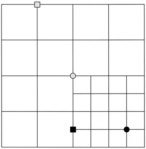
The mesh structure adopted is non-conforming, in the sense that we allow hanging nodes[27]. We
distinguish between four different node types; internal nodes, boundary nodes, hanging nodes and interface nodes. In the case of a uniformly refined mesh all nodes are either internal nodes or boundary nodes. In the case of non-uniformly refined meshes the nodes that lie at the interface of two levels of refinement are termed as either interface nodes or hanging nodes. Hanging nodes are nodes that exist only on the finer grids, while interface nodes exist on both the finer and next coarser grid (see Fig. 1). Standard second-order central difference schemes are used to approximate the first and second differentials of φ, U and θ, while a compact 9-point scheme has been used for the Laplacian terms in the phase equation as this has been shown to reduce mesh induced anisotropy effects[28 29, ]. The mesh data is stored in a quadtree data structure as in
[30].
(
φ θν ∇ + ∇ + ∇
=h EC U ET
E
)
(21)where h|ν| is the element size on the finest level of refinement and EC and ET are user-defined constants
which control the respective effect of the concentration and thermal fields relative to the phase-field. These
are compared to two tolerances, and . If, at any location within the domain the mesh is
refined at that location while conversely if the mesh is permitted to coarsen at that location.
Refinement and coarsening proceeds via a two step process. On the first sweep through the mesh the elements targeted for refinement (coarsening) based upon the gradient criterion are marked, and on the second sweep the marked elements are refined/coarsened. In order to guarantee that the solution is sufficiently resolved, a number, N
+ Tol
E
E
Tol−E
≥
E
Tol+−
≤
E
TolE
s, of extra (safety) layers of elements may be added to those marked by the
gradient criterion at each level. This helps to ensure that the interface region does not move out of the most refined area of the mesh during a given time-step. In addition we apply two further refinement rules;
● Two neighbouring elements should differ by at most one level of refinement.
● An element cannot be further refined once it has reached a user-defined maximum level of refinement.
The most commonly employed temporal discretization scheme utilised in phase-field modelling are explicit methods such as the Forward Euler scheme. Rewriting Equations (13)-(15) in operator form
(
)
⎟ ⎠ ⎞ ⎜ ⎝ ⎛ ∂ ∂ = ∂ ∂ ⎟ ⎠ ⎞ ⎜ ⎝ ⎛ ∂ ∂ = ∂ ∂ = ∂ ∂ t t F t t U t F t U U t F t U φ θ θ φ φ θ φ φ θφ , , , , , , , , , , (22)
the forward Euler scheme can be written as
(
)
(
)
(
)
⎥⎥ ⎥ ⎦ ⎤ ⎢ ⎢ ⎢ ⎣ ⎡ Δ = ⎥ ⎥ ⎥ ⎦ ⎤ ⎢ ⎢ ⎢ ⎣ ⎡ − ⎥ ⎥ ⎥ ⎦ ⎤ ⎢ ⎢ ⎢ ⎣ ⎡ + + + + + 1 1 1 1 1 , , , , , , , , k k k k k k k U k k k k k k k k k k t F U t F U t F t U U φ θ φ φ θ φ θ φ θ φ θ φ && (23)
The implementation of explicit methods is straight forward, but they suffer from a time-step restriction in order to ensure the stability of the discretization scheme, which is of the form
2 .h C t≤
where h is the minimum element size and for some non-linear PDE’s the value of C can be very small, leading to excessively small time steps on heavily refined grids. Moreover, we have shown elsewhere[ ]26 that for the complex equations considered here C = C(λ, Le, Δ) , with C varying from ≈ 0.3 at Le = 1 to C≤ 0.001 at Le = 500 at which point the tests to evaluate to C were terminated due to the extremely long computational time required to evaluate the explicit Euler method, despite Le = 500 still being significantly short of values typical of liquid metals.
In order to overcome these restrictions, implicit time stepping methods have been utilised here as these may be designed to be unconditionally stable. In particular, we have used the second order Backward Difference Formula (BDF2), which is an implicit linear 2-step method which, with a constant time step, Δt, takes the following form
(
)
(
)
(
)
⎥⎥ ⎥ ⎦ ⎤ ⎢ ⎢ ⎢ ⎣ ⎡ Δ = ⎥ ⎥ ⎥ ⎦ ⎤ ⎢ ⎢ ⎢ ⎣ ⎡ + ⎥ ⎥ ⎥ ⎦ ⎤ ⎢ ⎢ ⎢ ⎣ ⎡ − ⎥ ⎥ ⎥ ⎦ ⎤ ⎢ ⎢ ⎢ ⎣ ⎡ + + + + + + + + + + + − − − + + + 1 1 1 1 1 1 1 1 1 1 1 1 1 1 1 1 1 , , , , , , , , 2 1 2 2 3 k k k k k k k U k k k k k k k k k k k k k t F U t F U t F t U U U φ θ φ φ θ φ θ φ θ φ θ φ θ φ && (25)
The method leads to second order convergence in both time and space. It can be shown that the BDF2 method is A-stable[31], and is therefore used for stiff systems of differential equations. The advantage over one-step second order methods such as Crank-Nicholson, is that only one non-linear solve is required at each time-step. The (small) price that has to be paid for this computational efficiency is that the solutions from the previous two time-steps must be saved. Although highly dependant upon the problem, particularly the value of Le, convergence studies[ ]26 have shown that the BDF2 method permits time steps between 80 and
several hundred times that allowed by the explicit forward Euler method.
Utilising an implicit time discretization scheme the appropriate selection of Δt shifts from being a question of numerical stability to one of accuracy. For typical phase-field simulations growth starts from a small nucleus. The initial growth of the nucleus will typically be very rapid, although the inherent instability of the interface will lead to the formation of dendritic arms that will ultimately grow with a steady-state velocity. Consequently, an adaption of the time step in the BDF2 method is likely to efficient and leads to an adaptive time and space discretisation method. It can be shown that in order to ensure second order
(
)
(
)
(
)
⎥⎥ ⎥ ⎦ ⎤ ⎢ ⎢ ⎢ ⎣ ⎡ Δ = ⎥ ⎥ ⎥ ⎦ ⎤ ⎢ ⎢ ⎢ ⎣ ⎡ + + ⎥ ⎥ ⎥ ⎦ ⎤ ⎢ ⎢ ⎢ ⎣ ⎡ + − ⎥ ⎥ ⎥ ⎦ ⎤ ⎢ ⎢ ⎢ ⎣ ⎡ + + + + + + + + + + + + + − − − + + + 1 1 1 1 1 1 1 1 1 1 1 1 1 1 2 1 1 1 , , , , , , , , 1 ) 1 ( 1 2 1 k k k k k k k U k k k k k k k k k k k k k t F U t F U t F t U r r U r U r r φ θ φ φ θ φ θ φ θ φ θ φ θ φ && (26)
The choice of appropriate time steps is based upon a set of local error estimators
(
)
∞ −
+ − + +
+
= 1 1 1
1
k k k
k r r r
r
Dφ φ φ φ (27)
(
)
∞ −
+ − + +
+
= 1 1 1
1
k k k
U
k U rU rU
r r
D (28)
(
)
∞ −
+ − + +
+
= 1 1 1
1
k k k
k rr r r
Dθ θ θ θ (29)
Each of the error estimators is compared against a corresponding tolerance ( , , ) and if at any
time-step the local temporal error = min( , , ) ≤ the time step is accepted and the next
time-step is increased whereas if the step is rejected and retaken with a smaller time-step. The
rate at which the time-step should grow can be estimated from
φ Tol
D
D
TolUD
Tolθk
D
DTolφD
TolUD
TolθD
TolTol k
D
D
≥
p k Tol D Dr ⎟⎟ +
⎠ ⎞ ⎜⎜ ⎝ ⎛ = 1 1 (30)
where p is the order of the scheme, which is 2 for the BDF2 method.
(
)
(
)
(
k k k)
ijij k ij r r k ij ij k k k k ij k ij U F r U F 1 1 1 * 1 1 2 1 1 1 * 1 1 , , 1 , , + + + ∂∂ − + + + + + + ⎟⎠ ⎞ ⎜ ⎝ ⎛ ⎟ ⎠ ⎞ ⎜ ⎝ ⎛ + − − − = θ φ φ φ θ φ ω φ φ φ φ φ (31)
(
)
(
)
(
k k k)
ijU ij k ij r r k ij ij k k k U k ij k ij U F U U r U F U
U * 1 1 1
1 1 2 1 1 1 * 1 1 , , 1 , , + + + ∂∂ − + + + + + + ⎟⎠ ⎞ ⎜ ⎝ ⎛ ⎟ ⎠ ⎞ ⎜ ⎝ ⎛ + − − − = φ φ φ φ ω φ & & (32)
(
)
(
)
(
k k k)
ijij k ij r r k ij ij k k k k ij k ij F r F 1 1 1 * 1 1 2 1 1 1 * 1 1 , , 1 , , + + + ∂∂ − + + + + + + ⎟⎠ ⎞ ⎜ ⎝ ⎛ ⎟ ⎠ ⎞ ⎜ ⎝ ⎛ + − − − = φ φ θ θ θ φ φ θ ω θ θ θ φ θ & & (33) with
(
1 1 1)
(
1 1 1 1)
1* 1 2 1 , , , , , + + + + + + + + + + + Δ −
= k k k k k
k k k r r U t tF U
Fφ φ θ φ φ θ φ (34)
(
1 1 1)
(
1 1 1 1)
1* 1 2 1 , , , , , + + + + + + + + + + + Δ −
= k k k k k
U k k k U U r r U t tF U
F φ φ& φ φ& (35)
(
1 1 1)
(
1 1 1)
1* 1 2 1 , , , , + + + + + + + + + + Δ −
= k k k k
k k k r r t tF
Fθ θ φ φ& θ θ φ& θ (36)
where the evaluation of the derivatives of the descritisation operators with respect to the system variable is discussed in [26].
On the basis of the described smoothing and transfer operators a multigrid solver for adaptively refined meshes has been developed based on the Full Approximation Scheme[ ]27 (FAS) for resolving the non-linearity. The number of pre- and post-smoothing operations required for optimal convergence has been investigated within the context of phase-field simulation in [26, 32]. Based on that work we have used V-cycle iteration with 2 pre- and 2 post- smoothing operations.
Calculation of the Dendrite Tip Velocity and Radius of Curvature
The two most important parameters to come out of quantitative phase-field simulations are the curvature and velocity of the dendrite tip, which therefore need to be calculated with a high degree of accuracy. The calculation of both these quantities requires accurate estimation of the tip position, for which we use a high order inverse interpolation scheme.
For a dendrite arm growing along the x–axis, which consists of the discrete points xj, for j = 1,N, we are
seeking the value x* on the x-axis, for which φ(x*) = 0. The method adopted here is based on Newton forward differences, wherein
(
j j)
i
j x x
x
x*= +ϑ +1− (37)
where i is the order of the interpolation and
(
( *) ( ))
1 1 j j x x φ φ φ ϑ − Δ= (38)
⎟ ⎠ ⎞ ⎜
⎝
⎛ − − − Δ
Δ
= j j
j
x
x φ ϑ ϑ φ
φ φ
ϑ 1 1 2
2 2 ) 1 ( ) ( *) ( 1 (39)
(
)(
)
⎟ ⎠ ⎞ ⎜ ⎝⎛ − − − Δ − − − Δ
Δ
= j j j
j
x
x φ ϑ ϑ φ ϑ ϑ ϑ φ
φ φ
ϑ 1 1 2 2 2 2 3
3 6 2 1 2 ) 1 ( ) ( *) ( 1 (40)
(
)(
)
(
)(
)(
)
⎟ ⎟ ⎟ ⎟ ⎠ ⎞ ⎜ ⎜ ⎜ ⎜ ⎝ ⎛ Δ − − − − Δ − − − Δ − − − Δ = j j j j j x x φ ϑ ϑ ϑ ϑ φ ϑ ϑ ϑ φ ϑ ϑ φ φ φ ϑ 4 3 3 3 3 3 2 2 2 2 1 1 4 24 3 2 1 6 2 1 2 ) 1 ( ) ( *) ( 1 (41)where φ(x*) = 0 in this case and
j j
j φ φ
φ = −
Δ +1 (42)
j j j
j j
j φ φ φ φ φ
φ =Δ −Δ = − +
Δ2 +1 +2 2 +1 (43)
j j j j j j
j φ φ φ φ φ φ
φ =Δ −Δ = − + −
Δ + 2 +3 +2 +1
1 2
3 3 3 (44)
j j j j j j j
j φ φ φ φ φ φ φ
φ =Δ −Δ = − + − +
Δ + 3 +4 +3 +2 +1
1 3
4 4 6 4 (45)
(
)
(
2)
322 2
1 x y
y x K
∂ ∂ +
∂ ∂
= (46)
and hence the actual radius of curvature at the tip
K a
1
=
ρ (47)
However, the actual tip radius is often not suitable for comparison with theoretical results[ , , 20 28 33], as most
dendrite growth theories assume a parabolic tip shape. Therefore, the procedure from [20] is adopted for calculating the parabolic tip radius. We introduce a local Cartesian co-ordinate system (x, y), situated at the actual tip position where x is pointing along the growth direction. The form of the parabola is then described by
) (
2 0
2 x x
y =− ρ − (48)
where ρ is the parabolic tip radius and x0 is the effective tip location. A simple least-squares fit to the φ = 0
isoline is used to determine the optimum values for ρ and x0, which is applied over a fitting range
right left,
~x = x x (49)
Results
The phase-field model used here is formally identical to that derived in [22], where the ability of the model to yield quantitative predictions is extensively validated. For this reason we do not repeat the validation of the model derivation. We give below the results of some comparative simulations which were also run by [20, 22] which we use to confirm that the numerical implementation of the model described above performs as expected. Far more extensive validation of our numerical techniques are presented in [26]. Having established the validity of the numerical scheme employed we then move on to present the results of a set of simulations designed to investigate the selection of the dendrite tip radius and growth velocity as the
undercooling is increased. In particular, we examine the regime where the dendrite passes from being predominantly solutaly, to thermally, controlled at sufficiently high Lewis number that in so doing a radius minimum is encountered.
Equations (13)-(15) has been solved on the domain Ω = [-800, 800]2, with simulation parameters Δ = 0.55,
Mc∞ = 0.07, Le = 40, ε = 0.02, kE = 0.15. In order to simulate kinetic free growth Equ. (16) is used with
λ = 2, which leads to D = 1.253328. Since the Lewis number is set to 40 it follows that the thermal
diffusivity is α = 50.13311. The mesh refinement parameters have been set as EC = 0.75 and ET = 1.0. The
problem is solved using a maximum of 11 levels of refinement, giving a minimum h of 0.78. This is
equivalent, were a uniform mesh to have been used, of a mesh size which is 211× 211. The multigrid solver is
iterated until an absolute residual of 10-5 is reached and the tolerance on the adaptive time-stepping routine,
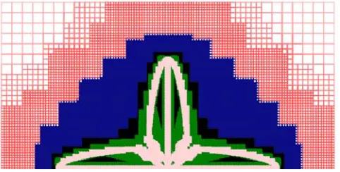
DTol, is set to 7.5 × 10⁻³. A typical mesh structure is shown in Fig. 2, while characteristic results for the
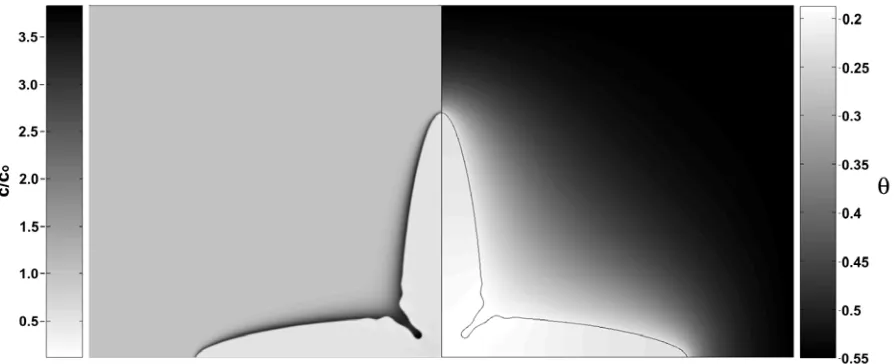
thermal (θ) and solutal fields (c/c∞) towards the end of the simulation are shown in Fig. 3, where boundary effects are already beginning to effect the simulation results. Even at this rather modest Lewis number it is clearly evident that the thermal field extends much more widely than the solute field. For this simulation the steady-state values of the growth velocity and dendrite tip radius are ρa/d0 = 16.34 and Vd0/α = 0.0040.
Fitting of a parabolic profile to the φ = 0 isoline, as described by Equ. (48) above, results in a parabolic radius of curvature ρ/d0 = 27.38 which also gives Vρ/2α = 0.0546. The fitting interval here is
10
-
,
100
~
x
=
−
, although keeping the fitting range constant and moving the fitting interval a further 40units to the right changes ρ by no more than 1.5%.
We believe that all of these results compare favourably with the results presented by Ramirez & Beckerman [Ref. 20, Figures 3-4]. Moreover, when the phase equation was solved directly in [20], using an explicit finite difference scheme, a severe grid dependence was found. This meant that small values of h
(typically h≈ 0.3) had to be used to get accurate solutions, with no converged solution at all being found for
h > 1. The problem was overcome by using a preconditioning technique, in which the phase equation was written in terms of a new variable ψ = tanh(φ/√2). In contrast, using an implicit multigrid solver no such h
dependence has been encountered. In numerical tests presented in [26] the variation in tip velocity was found to vary by no more than 5% as h was reduced from 0.78 to 0.097.
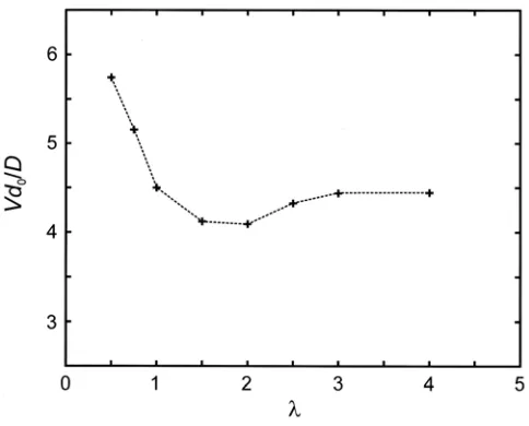
for λ = 8 this is W0 = 9.05d0, that is 28%-55% of ρa. Given that W0 is a measure of the width of the diffuse
interface it would not be surprising if the quality of the solution were to degrade as the width of the diffuse interface approached the actual radius of curvature of the dendrite tip. However, of more concern is the variation observed in the solution as λ is varied in the range 1-4, most notably a ≈40% decrease in the tip velocity as λ is decreased. As one of the fundamental properties of the thin-interface model is that the solutions should be independent of the mesoscopic interface width, this an effect that we have chosen to investigate further with the multigrid method reported here. Fig 4 shows the variation of the scaled velocity
Vd0/α as a function of λ and should be directly comparable to the solid line in [20, Fig. 5]. Unlike [20] who
observe a variation in Vd0/α of up to 25% between λ = 1 and λ = 4 we observe a much smaller variation of
no more than 10% over the same interval. However, the most notable effect is the sharp increase in Vd0/α
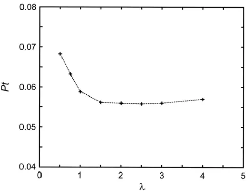
for λ < 1, which corresponds to the width of the diffuse interface being less than the capillary length. Fig. 5, which shows the Peclet number as a function of λ, would tend to confirm that this is a real effect. For
λ > 1.5, Pt is remarkably constant, with a mean value of 0.0563 ± 0.0005, but again for small values of λ a strong systematic increase is observed. However, as yet the exact origins for this variation are unknown.
We now move on to consider the variation of ρ as Δ is increased. Fig. 6 shows a family of plots of ρ against Δ calculated using the LKT[ ]7 model. The parameters used here are Mc∞ = 0.05, k
E = 0.30 and
σ* = 0.05. The curves clearly show that the depth of the predicted minimum is a strong function of Le, while
both the predicted minimum and maximum occur at lower values of Δ as Le is increased. It is apparent from Fig. 6 that the minimum value of Le at which we might reasonably expect to be able to observe a minimum in ρ is Le = 200, which accordingly is the value adopted in the phase-field simulations. The simulations are run on a domain of size Ω = [-1600, 1600]2, which is larger than the previous set of simulations as the higher
Lewis gives rise to a more extensive thermal boundary layer. A maximum of 12 levels of refinement are used, which as before gives a minimum h of 0.78, equivalent, were a uniform mesh to have been used, of a mesh size which is 212× 212. The other parameters used in the simulation are ε = 0.02 and λ = 1. This final
parameter has been chosen as a compromise between the anomalous behaviour observed in Fig. 4 and the need to keep the ratio of the interface width to the solute boundary layer width (W0V/D) less than or of order
values of Δ between 0.1 and 0.8 are shown in Figures 7 & 8 respectively. The velocity shows a simple power law dependence on Δ of the form V ∝Δβ, which has been widely reported as being the case in
experimental velocity-undercooling studies [see e.g. 34, 35], where β is a material dependant constant which is typically in the range 2.0-3.5. The least-squares value of β found for the simulations reported here is 2.39. As is apparent from Fig. 8 a clear radius minimum is observed in the data, albeit at a rather higher value of Δ
than would have been expected from the LKT theory. There is however, no evidence of a velocity maximum, despite the fact that from the LKT prediction this should occur well below the maximum Δ
studied here of 0.8. Yet higher values of Δ have not been studied as the value of W0V/D for Δ = 0.8 is 1.6,
and although this is probably still acceptable[ ]20, significantly higher values may lead to computational artefacts in the solution.
In order to better understand the observed results we have calculated σ* as a function of Δ, using both the LGK and LKT definitions. In both models this would be expected to be a material-dependant constant, although for both pure thermal and pure solutal growth in 2-dimensions[ ]20 and pure thermal growth in
3-dimensions[ ]28 σ* appears to decrease approximately linearly with increasing Peclet number, with the
coupled thermo-solutal model of [20] showing a rather steeper decrease in σ*. In order to calculate σ* in such a way that it is independent of the Ivantsov solution when Δc is evaluated the following procedure has been adopted from [20]. Δc can be written as
i E i
U k U c
) 1 ( 1+ − =
Δ (50)
where Ui is the value of U ‘frozen in’ at the interface (NB there is an error in [20] which meant that Equ. (50)
appeared as Ui[1+(1-kE)Ui]). The correct form is as shown above, although there is no evidence this is
anything other than a typesetting error in [20], the results presented being consistent with the correct form of the equation being used). Ui may either be read directly from the simulations or evaluated from
∞
− −
− =
Mc d
U a i
i ε ρ θ
) 15 1 (
where θi is the value of θ at the interface. The latter of the two methods has been used here, with θi being
evaluated at φ = 0.9, although as the solid is essentially isothermal the value obtained does depend critically upon the value of φ selected.
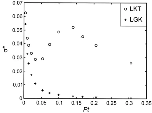
The results of calculating the selection parameter, σ*, are shown in Fig. 9, for both the LGK and LKT basis. As in [20] we find that as Pt→ 0, σ* approaches a value of approximately 0.07, which is consistent with it being independent of the alloy concentration in the low undercooling limit (note that although we have used different material parameters this should not matter as in the limit Pt→ 0, σ* should depend only upon ε, which is the same as in [20]). However, unlike [20] we find at higher Lewis number very significant difference in behaviour between the LGK and LKT definitions of σ*. On the LGK definition σ* drops monotonically, reaching at the highest Peclet numbers studied a very low value, around 0.0006. In fact, above Pt = 0.15, σ* on the LGK definition is very close to varying in direct proportion to 1/Pt. In contrast, on the LKT definition, σ* varies non-monotonically, showing a minimum at Pt = 0.0325 (Δ = 0.4), co-incident with the minimum in ρ, while the maximum in σ* occurs at Δ = 0.65 (Pt = 0.14), an undercooling which does not correspond to any obvious feature in the plot of ρ against Δ.
However, the physical significance of these results is far from clear. One would have expected a priori
the LKT definition of σ* to be superior due to the high undercooling corrections effected by the inclusion of the terms ξT and ξc. Indeed, the inclusion of the ξ parameters keeps σ* (on the LKT definition) constant to
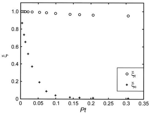
within a factor of ≈ 2, while on the LGK definition σ* varies by over two orders of magnitude. The variation of the ξ parameters with Pt is shown in Fig. 10, showing in particular that across the range of undercoolings studied here ξc varies from close to 1 (solute dominated growth) to essentially zero (no solute effects).
However, from a quantitative point of view a variation of a factor of two is still significant, particularly when it is borne in mind that in the most widely used method for estimating the characteristic microstructural length scale for rapid solidification processes is still the use of the LKT model with a constant σ* estimated from the anisotropy in the zero Peclet number limit.
Summary & Discussion
time-stepping and multigrid methods. Moreover, by using a formulation of the non-isothermal problem based on the thin-interface model these results should be independent of the width assumed for the diffuse interface, giving them a quantitative validity which cannot be claimed by other formulations of the non-isothermal problem. We have used this model to investigate the behaviour of the dendrite tip radius and growth velocity as a function of undercooling for a dilute alloy at a Lewis number of 200, confirming theoretically for the first time that the dendrite tip radius does indeed pass through a minimum with
increasing undercooling. However, up to the highest undercooling studied (Δ = 0.8) no evidence of a radius maximum has been observed. The radius selection parameter, σ*, has been calculated as a function of undercooling and this is shown to be far from being constant, with approximately a factor of two variation observed (LKT definition of σ*) over the range of undercoolings studied. This highlights the potential limitations of assuming constant σ* in simple analytical models of solidification to predict dendrite length scales.
References
1. D.P. Corrigan, M.B. Koss, J.C. LaCombe, et al., Phys. Rev. E60 (1999) 7217.
2. U. Bisang & J.H. Bilgram, Phys. Rev. E54 (1996) 5309.
3. G.P. Ivantsov, Doklady Akademii Nauk SSSR58 (1947) 567.
4. W.W. Mullins & R.F. Sekerka, J. Appl. Phys. 33 (1964) 444.
5. J. Lipton, M.E. Glicksman & W.Kurz, Mater. Sci. Eng.65 (1984) 57.
6. J. Lipton, M.E. Glicksman & W.Kurz, Metall. Trans. A18 (1987) 341.
7. J. Lipton, W. Kurz & R. Trivedi, Acta Metall. 35 (1987) 957.
8. R. Willnecker, D.M. Herlach & B. Feuerbacher, Phys. Rev. Lett.62 (1989) 2707.
9. S.C. Huang & M.E. Glicksman, Acta Metall.29 (1981) 701.
10. D.A. Kessler, J. Koplik & H. Levine, Adv. Phys.37 (1988), 255.
11. Y. Pomeau & M. Ben-Amar, in ‘Solids far from equilibrium’ pp. 365-431, Cambridge University Press, 1992.
12. A.M. Mullis & R.G. Cochrane, Acta Mater. 49 (2001) 2205.
13. J.S. Langer, in ‘Directions in condensed matter physics’ (eds. G. Grinstein & G. Mazenko), 1986, pp. 164-186, World Science.
15. O. Penrose & P.C. Fife, Physica D43 (1990) 44.
16. R. Kobayashi, Physica D63 (1993) 410.
17. A.A. Wheeler, B.T. Murray & R.J. Schaefer, Physica D66 (1993) 243.
18. I. Loginova, G. Amberg & J. Aagren, Acta Mater. 49 (2001) 573.
19. J.A. Warren & W.J. Boettinger, Acta Metall. Mater. 43 (1995) 689.
20. J.C. Ramirez & C. Beckermann, Acta Mater. 53 (2005) 1721.
21. C.W. Lan, Y.C. Chang & C.J. Shih, Acta Mater.51 (2003) 1857.
22. J.C. Ramirez & C. Beckermann, Phys. Rev. E69 (2004) 051607.
23. A. Karma, Phys. Rev. Lett.87 (2001) 115701.
24. G. Horvay & J. W. Cahn, Acta Metall.9 (1961) 695.
25. M. J. Aziz, J. Appl. Phys., 53 (1982) 1158.
26. J. Rosam, ‘A fully implicit, fully adaptive multigrid method for multi-scale phase-field modelling’, Ph.D. thesis, University of Leeds, 2007.
27. U. Trottenberg, C. Oosterlee & A. Schüller, Multigrid, Academic Press, 2001. 28. A. Karma & W.J. Rappel, Phys. Rev. E57 (1998) 4323.
29. B. Echebarria, R. Folch, A. Karma & M. Plapp, Phys. Rev. E70 (2004) 061604.
30. N. Provatas, N. Goldenfeld & J. Dantzig, J. Comp. Phys. 148 (1999) 265.
31. W. Hundsorfer & J.G. Verwer, Numerical Solution of Time-Dependant Advection-Diffusion-Reaction Equations, Springer-Verlag, 2003.
32. J. Rosam, P.K. Jimack & A.M. Mullis, J. Comp. Phys.225 (2007) 1271.
33. X. Tong, C. Beckermann, A. Karma, & Q. Li, Phys. Rev. E63 (2001) R49.
34. K. Eckler & D.M. Herlach, Mater. Sci. Eng.A128 (1994) 159.
Fig. 3. Thermal and solutal fields around a dendrite growing with a Lewis number of 40 (the solid-liquid
Fig. 4. Variation of the dimensionless dendrite growth velocity as a function of the coupling parameter, λ.
Fig. 6. Dendrite tip radius as a function of undercooling for Lewis numbers in the range 50-1000 as
Fig. 7. Dimensionless dendrite growth velocity as a function of undercooling, showing very close agreement
Fig. 8. Dimensionless dendrite tip radius as a function of undercooling, showing a clear minimum at a
Fig. 9. Radius Selection parameter calculated on (a) the LGK (no high undercooling corrections) and (b) the
Fig. 10. Values of the thermal and solutal correction parameters (ξt and ξc) used in the LKT calculation of