Swept boundary layer transition

Fluids Engineering Research Group

School of Engineering

Swept Boundary Layer Transition

by

Adam Yuile

Thesis submitted in accordance with the requirements of the

University of Liverpool for a PhD degree

i

Statement of Originality

This thesis has been submitted by Adam Yuile to be examined as part of a PhD research degree for the School of Engineering at the University of Liverpool.

The research material reported herein was carried out solely by the author, under the primary supervision of Dr. Mark W. Johnson, for the Fluids Engineering Research Group at the University of Liverpool over a period of 4 years, starting in October 2009.

ii

Acknowledgements

The first person I wish to express my gratitude to is Dr. Mark W. Johnson for his invaluable

supervision, encouragement and enthusiasm to help deliver this project to completion. Dr. Mark W. Johnson is not only an excellent source of knowledge, particularly on boundary layer transition, but also radiates an infectious happiness which brings fun into the workplace. I will forever be grateful for his support in allowing me to suspend my studies for a single semester placement in Hong Kong.

I must also thank those responsible at the University of Liverpool for giving me the opportunity to conduct my studies here and, despite my vociferous grumblings about long delivery times, for eventually producing everything I needed to adequately conduct research in boundary layer transition. On the issue of delays I would like to extend a special thanks to Prof. Ieuan Owen

(former secondary supervisor) for the help he provided in our attempts to realise the manufacture of equipment as quickly as possible.

In terms of support from technical staff I would like to extend thanks to Derek Neary, John Curran

and Steve Bode, as well as Marc Bratley, Bob Seamans and Martin Jones who (between them) helped manufacture and assemble the test sections on the wind tunnel for each pressure gradient, as well as the traverse and all its associated ancillary equipment.

I’ve been a member of the Fluids Engineering Research Group for 4 years and have seen a lot of students graduate from within, in addition to having shared discussions with them on our research projects and social matters. Some people I’ve been fortunate enough to work with in this group were (my former housemate) Dr. Chris Kaaria, Dr. James Forrest, Dr. Sean Malkeson, Dr. Mohit Katragadda, Dr. Dimitris Tsovolos, Dr. Richard Whalley and Miss. Siân Tedds (soon to be doctor!).

iii

Abstract

Boundary layer transition has been investigated for incompressible three-dimensional mean flows on a flat plate with a 60° swept leading edge for a nominally zero, a positive, and a negative pressure gradient for three freestream turbulence intensities using a low speed blower tunnel with a 1.22 x 0.61 m working section at the University of Liverpool. The freestream turbulence intensities were generated using grids upstream of the leading edge, producing turbulence levels of approximately 0.2 %, 1.25 % and 3.25 %.

For each of these nine (3 x 3) test cases detailed boundary layer traverses were obtained at ten streamwise measurement stations, at a fixed spanwise location, using single-wire constant temperature hot-wire anemometry techniques and digital signal processing. The location for the onset and end of transition was obtained for each case, in terms of distance from the leading edge and local momentum thickness Reynolds number. These results are compared with the 2-D unswept empirical transition correlations of Abu-Ghannam and Shaw (1980) and the differences in the results between the two flows are highlighted. It was found that transition starts and ends earlier than for similar unswept flows, complementing the transition observations of Gray (1952) for swept wings.

iv

observed in flow visualisations and direct numerical simulation studies of pre-transitional boundary layers.

Additionally it was also found that the numerical receptivities to freestream turbulence were highest for the positive pressure gradient and, in contrast, lowest for the negative pressure gradient – a similar finding to that in 2-D boundary layers. Transition was seen to commence prior to the advent of the intended non-zero pressure gradients in the experiments and thus direct comparisons are not strictly available.

v

Contents – Swept Boundary Layer Transition

Statement of Originality ... i

Acknowledgements ... ii

Abstract ... iii

Contents – Swept Boundary Layer Transition ... v

Nomenclature ... ix

Abbreviations ... xii

1 Chapter 1 – Introduction ... 1

2 Chapter 2 – Literature Review of Swept Boundary Layer Transition ... 4

2.1 Introduction to Boundary Layer Transition ... 4

2.2 Fundamental Boundary Layer Parameters ... 5

2.3 Boundary Layer Transition Processes ... 9

2.3.1 Intermittency Effect ... 15

2.3.2 Influence of Freestream Turbulence on Transition – Intensity and Length Scale ... 18

2.3.3 Influence of Pressure Gradient on Transition ... 19

2.4 Boundary Layer Theory ... 22

2.4.1 Laminar Boundary Layers ... 22

2.4.2 Transitional Boundary Layers ... 23

2.4.3 Turbulent Boundary Layers ... 25

2.5 3-D Boundary Layers ... 30

2.5.1 Falkner-Skan-Cooke Boundary Layer Example ... 33

2.5.2 Instability Mechanisms for Swept Transition ... 37

2.5.3 Receptivity in 3-D Boundary Layers ... 42

3 Chapter 3 – Experimental Procedures, Apparatus and Data Processing ... 44

3.1 Blower Wind Tunnel ... 44

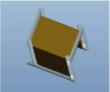
3.2 Swept Flat Plate and Leading Edge Control Flap ... 49

3.3 Turbulent Grids ... 55

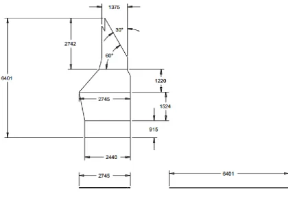
3.4 Section Sidewall Profiles and Design ... 58

3.5 Inclined Manometer ... 67

3.6 Cathetometer ... 69

vi

3.8 Pitot-Static Tube (Validyne) ... 75

3.9 Constant Temperature Hot-Wire Anemometry – CTA Boxes (54T30 & StreamlinePro) ... 76

3.9.1 54T30 Miniature CTA Experimental Configuration ... 77

3.9.2 StreamLine Pro CTA Experimental Configuration ... 79

3.10 Main Data Acquisition Card (USB 6210) ... 81

3.11 Static Pressure Tappings ... 83

3.12 Hot-Wire Systems, Calibration and Corrective Procedures ... 85

3.12.1 Advantages and Disadvantages of Hot-Wire Anemometry Systems ... 86

3.12.2 Hot-Wire Calibration ... 88

3.12.3 Wall-Proximity Effect and Initial Probe Height... 90

3.12.4 Corrective Procedures for Ambient Drift ... 92

3.13 Data Processing ... 95

3.14 Intermittency Algorithm ... 96

3.14.1 High Pass Filter Setting for Intermittency Algorithm ... 98

3.14.2 Window Size for Intermittency Algorithm ... 100

3.14.3 Residence Time for Intermittency Algorithm ... 101

3.15 Experimental Procedure ... 101

3.16 Measurement Uncertainties ... 104

3.16.1 Calibration Uncertainty ... 105

3.16.2 Uncertainty in Alignment of Probe ... 105

4 Chapter 4 – Swept Boundary Layer Transition Experimental Results ... 107

4.1 Streamwise Static Pressure Distributions ... 107

4.2 Nominally Zero Pressure Gradient (GxZ) ... 111

4.2.1 Wall Normal Profiles under Zero Pressure Gradient (G0Z) ... 111

4.2.2 Streamwise Parameters under Zero Pressure Gradient (G0Z) ... 118

4.2.3 Flow Angles (G0Z) ... 124

4.2.4 Falkner-Skan-Cooke Comparisons (G0Z) ... 128

4.2.5 G1Z ... 134

4.2.6 G3Z ... 136

4.3 Positive Pressure Gradient (GxP) ... 138

4.3.1 G0P ... 138

4.3.2 G1P ... 143

4.3.3 G3P ... 146

vii

4.4.1 G0N ... 148

4.4.2 G1N ... 151

4.4.3 G3N ... 152

4.5 Collective Analysis of Results ... 155

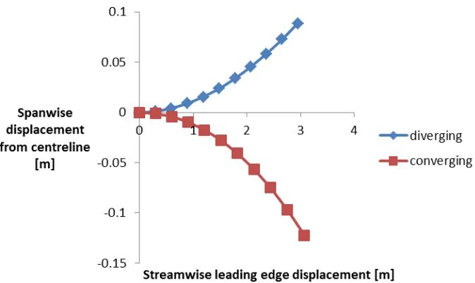
4.6 Spanwise Flow Quality Issues ... 159

4.7 Receptivities of Pre-Transitional Boundary Layers (Experiments) ... 165

4.7.1 ZPG Receptivities ... 166

4.7.2 PPG Receptivities ... 169

4.7.3 NPG Receptivities ... 170

5 Chapter 5 – Crossflow Boundary Layer Receptivity Code ... 172

5.1 3-D Steady Code ... 172

5.1.1 3-D Steady Code Results ... 174

5.2 3-D Unsteady Code ... 178

5.2.1 3-D Unsteady Code Results ... 184

5.3 Comparisons between Numerical and Experimental Results ... 192

5.3.1 Non-Dimensional Numerical Receptivities ... 194

5.3.2 Non-Dimensional Experimental Receptivities ... 199

5.4 Comparisons with 2-D Results ... 204

6 Chapter 6 – Conclusions and Suggestions for Future Work ... 206

6.1 Conclusions ... 206

6.2 Recommendations and Suggestions for Future Work ... 207

7 List of Tables ... 210

8 List of Figures ... 211

9 References ... 217

10 Appendix A – OpenFOAM and ANSYS Fluent Receptivity ... 228

10.1 Derivation of Real Inflow Velocity Components ... 228

10.2 OpenFOAM Case Library Files ... 230

10.3 OpenFOAM Results ... 247

10.4 NACA 0002 Test Case ... 250

11 Appendix B – LabVIEW Codes (Experimental) ... 256

11.1 Record Wire Velocities and King’s Law with Temperature Correction ... 256

11.2 U and Delta Seek ... 258

11.3 Intermittency ... 259

viii

ix

Nomenclature

Symbol Function Dimensions

A King's law coefficient

a overheat ratio

ax streamwise frequency rad/m

ay wall normal frequency rad/m

az spanwise frequency rad/m

B King's law coefficient

Cf skin friction coefficient

E hot-wire voltage V

Ecorr temperature corrected hot-wire voltage V

g acceleration due to gravity m/s²

Gx streamwise coordinate (unswept) m

Gy wall-normal coordinate (unswept) m

Gz spanwise coordinate (unswept) m

h local height of tunnel section m

h0 inlet height of tunnel section m

H shape factor

L characteristic length (for Reynolds number) m

Lx streamwise coordinate (swept - normal to leading edge) m

Ly wall-normal coordinate (swept) m

Lz spanwise coordinate (swept - parallel with leading edge) m m Hartree parameter

n King's law coefficient

n arbitrary parameter for skew angle cosine fit

p surface static pressure Pa

P ambient pressure Pa

R ideal gas constant J/kgK

R receptivity

Ruv u’v’ receptivity Rvw v’w’ receptivity

Ramb wire ambient resistance Ω

Rec corrected Reynolds number (Wills method) Recf critical crossflow Reynolds number

Rem measured Reynolds number (Wills method) Rex streamwise Reynolds number

Reδ boundary layer thickness Reynolds number Reδ* displacement thickness Reynolds number

Reθ momentum thickness Reynolds number

Rw wire hot resistance Ω

̅̅̅̅̅ _{integral averaged receptivity (fixed streamwise frequency)}

x

Tl laminar signal time s

TI turbulence intensity %

Tt turbulent signal time s

Tref calibration reference temperature K

Tw sensor wire temperature K

u streamwise velocity m/s

ucorr corrected velocity (Wills method) m/s

u' standard deviation in streamwise velocity m/s

U0 inviscid inlet velocity m/s

U1 inviscid local velocity m/s

freestream velocity m/s

uτ friction velocity m/s

v wall-normal velocity m/s

v' standard deviation in wall-normal velocity m/s

w spanwise velocity m/s

w' standard deviation in spanwise velocity m/s

x0 datum location for FSC profile m

xt location for start of transition (Narasimha) m

streamwise location for 25% intermittency m streamwise location for 75% intermittency m

α roof convergence angle °

β perturbation decay rate m-1

γ intermittency %

γ1 raw intermittency %

γ2 Wills corrected intermittency %

δ boundary layer thickness m

δ* displacement thickness m

θ momentum thickness m

λ skew angle (probe angular position) °

λ arbitrary Narasimha parameter m

Ω non-dimensional temporal frequency

Ωx non-dimensional x frequency Ωy non-dimensional y frequency Ωz non-dimensional z frequency

μ fluid dynamic viscosity kg/ms

μt artificial eddy/turbulent viscosity kg/ms

ν fluid kinematic viscosity m²/s

ρ density kg/m³

τ turbulence intensity (u'/u) - local mean %

τw near-wall shear stress Pa

φ leading edge sweep angle °

χ mean flow direction °

ψ stream function m²/s

xi

ωx spatial x frequency rad/m

ωy spatial y frequency rad/m

xii

Abbreviations

Abbreviation Long name

ADC Analogue to Digital Converter

ANSI American National Standards Institute

ASCII American Standard Code for Information Exchange

ASU Arizona State University (US)

CFL Courant-Friedrichs-Lewy

CNC Computer Numerical Control

CTA Constant Temperature Anemometer

DAQ Data Acquisition (USB-DAQ)

DLR German Aerospace Center (Germany)

DNS Direct Numerical Simulation

DSO Digital Storage Oscilloscope

ERCOFTAC European Research Community On Flow, Turbulence and Combustion

FFT Fast Fourier Transform

FP Flat Plate

HWA Hot-Wire Anemometry

ITAM Institute of Theoretical and Applied Mechanics (Russia)

LabVIEW Laboratory Virtual Instrument Engineering Workbench

MATLAB Matrix Laboratory

MFA Mean Flow Angle

MPI Message Passing Interface

NACA National Advisory Committee for Aeronautics

NAL National Aerospace Laboratory (Japan)

ODE Ordinary Differential Equation

NPG Negative Pressure Gradient

PPG Positive Pressure Gradient

RANS Reynolds-Averaged Navier-Stokes Equations

TS Tollmien-Schlichting

TTL Transistor-Transistor Logic

USB Universal Serial Bus

VI Virtual Instrument (LabVIEW)

1

1

Chapter 1 – Introduction

The onset of turbulent structures in shear flows has intrigued investigators for more than a century (Kachanov (1994)). A tremendous volume of effort continues to be directed towards improving the understanding of the inception and evolution of turbulent structures in boundary layer flows, owing to the potential improvements, in terms of performance and efficiency, for the likes of aircraft wings and gas turbine engines. This is particularly important given that the majority of flows occurring in nature and engineering are turbulent (Tennekes and Lumley (1972)). In Tempelmann (2011) it is stated that around 20% of the drag on modern aeroplanes can typically be attributed to skin friction acting on the wing surfaces alone. However, in Kohama (1987) it was stated that the boundary layers over swept wings are generally turbulent and can account for up to 50% of the total drag on an aircraft at cruise. The difference between these two quoted figures can perhaps be attributed to the increased use of natural laminar flow wings. The primary advantage of sweeping a wing (backwards or forwards) is a net reduction in wave drag, Pearcey (1962), with the compromise of less favourable stall characteristics, which must be managed accordingly.

Furthermore, in gas turbine engines, the boundary layer flow on the turbomachinery blade surfaces is said to be transitional for 50 – 80 % of the chord length, Brandt (2003). For turbomachinery designers it is important to accurately quantify the fraction of blade chord that is turbulent as this will not only have implications in terms of potential losses through increased skin friction, but also in terms of being able to reliably quantify the cooling requirements for the high pressure turbine in a large axial turbofan for example, owing to the higher heat transfer rates associated with turbulent flows (through Reynolds analogy, see Anderson (2010)).

2

Sweep is commonly used by designers of turbomachinery, see the backswept centrifugal impeller of Eckardt (1979) for example, to control tip Mach numbers and to optimise aerothermodynamic performance.

Technically speaking, a boundary layer is a momentum deficient region of flow in a viscous fluid which is manifested in the immediate vicinity of a solid surface (such as a duct wall or fuselage skin) as that fluid translates with respect to the surface, which itself may or may not itself be at

rest. Boundary layer transition, however, can be considered as the process between laminar and turbulent parts of the boundary layer. This robust description of transition, as a process, can be broken down into forward transition (laminar to turbulent) or reverse transition (turbulent to laminar) also known as (re)laminarisation. Laminar flow (from the Latin “lamina” meaning layer, sheet or leaf) is characterised as being ordered, predictable and layered - Brandt (2003). Turbulent flow or turbulence, on the other hand, is characterised as being chaotic and inherently three-dimensional (Versteeg and Malalasekera (2007)).

There are many examples of generic boundary layer transition work which has been conducted both internally (at the University of Liverpool) and throughout the world (example research programmes include ASU, DLR, KTH, ITAM and NAL), an excellent review of such experimental studies in swept transition is provided by Bippes (1999). In relatively recent times this work has been primarily focused on two-dimensional flat plates from which there has been considerable return on

investment which has translated to both empirical correlations for predicting the start and end of transition (e.g. Abu-Ghannam and Shaw (1980)) and physical models of transition, such as the receptivity transition model of Johnson and Ercan (1996).

3

inherited for this research, to study relaminarisation with the justification for 60° of sweep being that the effects were likely to be readily observable at such a high angle. The latter author, Riley (1985), highlighted a ‘paucity’ in terms of the amount of work in this area present within the research community, but this has subsequently been addressed in the intervening three decades. Nevertheless there still would appear to be a shortage of research specific to bypass transition in 3-D mean flows, hence this area is the focus of this thesis, with the main deliverable objective being to quantify boundary layer receptivity in swept flows and to highlight the underlying physical

differences with respect to unswept 2-D flat plate flows.

The layout of this thesis is as follows Chapter 2 – Literature Review of Swept Boundary Layer Transition offers a literature review of the general boundary layer transition process and attempts to provide a brief overview of the current state of the art in terms of most of the concepts and physical knowledge mostly specific to the case of transition on swept flat plates. More detailed descriptions and analyses of the important parameters and flow features observed in each of the flow regimes are also discussed. Chapter 3 – Experimental Procedures, Apparatus and Data Processing as the name suggests covers the methodologies from which the transition experiments were conducted and how the resulting data acquired was processed. Chapter 4 – Swept Boundary Layer Transition Experimental Results and Chapter 5 – Crossflow Boundary Layer Receptivity Code

4

2

Chapter 2 – Literature Review of Swept Boundary Layer Transition

2.1

Introduction to Boundary Layer Transition

The transition from laminar to turbulent flow is fundamental for understanding fluid dynamics, particularly given that the overwhelming majority of engineering fluid field problems, both internal and external, involve turbulence (Cant (2002)) and the genesis of such research is attributed to Osbourne Reynolds, as stated by Schlichting (1968). In order for transition to turbulent flow to take place there need to be circumstances which allow for breakdown in stability. In general terms the probability of breakdown to turbulence is proportional to the ratio of inertial and viscous forces, a non-dimensional parameter which is attributed to Osborne Reynolds as being the Reynolds number (Equation 2-1) owing to his work in the late 19th century on tube flows (Reynolds (1883)). One of these experiments involved adding streaks of “highly coloured water” (dye) to the colourless water and tracking the development of the flow patterns downstream, where the initially laminar streaks were (after some critical distance) observed to curl up and the dye was observed to diffuse

throughout the water in the pipe, in other words transition as we know it today was witnessed.

5

Reynolds was also aware of the importance of the incoming flow and found that the critical Reynolds number effectively was inversely proportional to the magnitude of the disturbances of the inlet flow. Similarly, in terms of the classical literature, in 1914 Ludwig Prandtl, often termed the ‘father of modern aerodynamics’, published his paper detailed his experiments with spheres, demonstrating both laminar and turbulent regimes and furthermore highlighting the problem of separation and that in such cases the overall drag is governed by the transition - Prandtl (1914) and reported in Schlichting (1968).

Equation 2-1

In the field of transition it is no longer possible to be utterly comprehensive, given the rapid expansion of knowledge which is constantly occurring, and the time span for which the subject has already been intensely studied. As such, this thesis tackles the specific case of incompressible boundary layer transition over swept flat plate topologies and hence, the literature review is

restricted to general transition theories and a concise literature review of swept flat plate transition, which will naturally draw content from transition studies on swept wings, given the overlap between the two sub-genres and the commercial appeal of such research in aerospace.

2.2

Fundamental Boundary Layer Parameters

6

Figure 2-1 - Two dimensional flat plate boundary layer flow depicting freestream velocity, local velocity components, boundary layer thickness, freestream approach flow and typical coordinate system, from Andersson (1999)

As previously mentioned this section discusses the fundamental parameters of boundary layer theory and those which derive from what’s known as the momentum integral equation (Schlichting and Gersten (2000)), known as the boundary layer integral parameters;

• Freestream velocity, - the freestream velocity, in an ideal scenario, equates to the velocity upstream of a particular object under consideration, such as an automobile model placed on a rolling road in a wind tunnel under test conditions. See the approach flow indicated in Figure 2-1.

• Boundary layer thickness, δ – the boundary layer thickness is defined as the normal

7

typical value for δ on the bonnet of a car travelling at 100 km/h is approximately 1 mm (Andersson (1999))

• Displacement thickness, – this parameter (Equation 2-2) equates to the offset through which a wall boundary would have to be displaced, normal to the direction of the potential flow, proportional to the reduction in volumetric flow rate of an inviscid fluid caused by the retardation due to viscosity in the boundary layer. In other words it’s an index proportional to the ‘missing mass flow’, Anderson (2010).

∫ ( ) Equation 2-2

• Momentum thickness, θ – similarly to the displacement thickness, the momentum thickness (Equation 2-3) is a representation of the decrement in the flow of momentum accounted for by the presence of the boundary layer.

∫ ( ) Equation 2-3

• Shear stress (wall), Equation 2-4; shear stress exists where there is a velocity gradient across streamlines (Anderson (2010)) and has the most significant effect where the

8

(

) Equation 2-4

• Skin friction coefficient, Cf – the skin friction coefficient (Equation 2-5) represents a non-dimensionalised version of the shear stress near the wall, normalised by the dynamic pressure of the adjoining freestream velocity. In practical terms it is a representation of the friction generated during the interaction of the air and the respective wall surface. The skin friction coefficient is markedly different for laminar and turbulent flows, owing to the larger velocity gradients and therefore shear stresses present in the latter regime.

Equation 2-5

• Shape factor, H – The shape factor of a boundary layer is defined as the ratio of the

displacement and momentum thicknesses - Equation 2-6. In practical terms the shape factor can be used as an indicator for characterising properties of the flow. For example in a 2-D laminar boundary layer (under zero pressure gradient conditions) the shape factor is around 2.6 and 1.3 - 1.4 for turbulent flows.

Equation 2-6

9

that from the point of view of the intermittency factor, that fully turbulent flow can in some sense be considered as a saturated transitional one. This is a point of view which is

supported by the fact that with sufficient stabilisation a fully turbulent flow can be relaminarised, where one will observe a drop in the intermittency.

Equation 2-7

2.3

Boundary Layer Transition Processes

Many experiments return boundary layer profiles which are laminar, transitional and fully turbulent in nature. As such many of the characteristics and important flow structures are briefly discussed in the following sections, where they are later identified and analysed in specific results in Chapter 4 and Chapter 5. This review only provides a brief overview of general transition theory but also attempts to provide guidance as to where the interested reader would be able to find out more in-depth analyses regarding these respective structures and characteristics.

10

Figure 2-2 - Transition paths following receptivity (Saric et al. (2002))

The following represents a description of what is known as the ‘natural’ transition process which corresponds to path A in Figure 2-2.

11

Thereafter an overview of path E (‘bypass’) transition is provided. Consideration of these two paths will provide a good overview of the transition process less the potential transition triggering

phenomenon of transient growth where transition can occur even if the exponentially growing perturbations are damped, see Brandt (2003) for example.

Natural transition on a 2-D flat plate (Path A) proceeds through the following stages;

 Receptivity – receptivity is the initial phase of transition and concerns the transformation of freestream disturbances into small perturbations within the boundary layer, hereafter the growth (or decay) of these perturbations will depend on the base flow and the nature of the disturbance, with respect to its characteristic frequencies and propagation direction.

 Primary modes – these modes of growth apply when the perturbations are sufficiently small that the disturbances can grow (or decay) in accordance with linear stability theory. An example of such a primary mode is Tollmien-Schlichting waves which propagate in the streamwise direction on a 2-D unswept flat plate, whereas in swept flows crossflow instability modes propagate in the spanwise direction.

 Secondary mechanisms (spanwise vorticity and 3-D breakdown, see Figure 2-3) – some primary instability modes can eventually grow to such an extent that the linear theories governing their growth are no longer physically applicable. Furthermore the magnitudes of the disturbances become so large that they significantly distort the mean flow which can lead to inflection points in the velocity profile, and hence an absolute instability in the boundary layer, which will rapidly lead to the next stage of transition - breakdown into turbulence.

12

Depending on the transition path some of these stages are said to be skipped/bypassed but there is evidence to say that each of the mechanisms is present, in some form or another, albeit at negligible intensities with respect to the dominant mechanism, see for example Hughes and Walker (2001) who observed TS activity in their spectral analysis of flows with upstream streaky structures which would normally correlate with the observations of bypass transition. In Andersson (1999) it is claimed that streamwise streaks are ubiquitous in transitional boundary layers, furthermore Klebanoff et al. (1962) were able to show that the onset of three-dimensionality is rapidly followed by the breakdown of the laminar flow.

The approximate freestream turbulence intensity for digitally switching between natural and bypass paths is usually considered to be 1% (Mayle (1991)) but as will be discussed in the following sub-sections, and indeed in other chapters, transition is affected heavily by more than just the turbulence intensity – pressure gradient and turbulence length scale to name just two additional parameters.

An equation describing the linear stability of parallel shear flows, known now as the Orr-Sommerfeld equation, was first presented by Orr (1907) and then Sommerfeld (1908), where the equation was considered to be derived independently, hence the shared attribution. This equation was an

enhancement of the approach devised by Rayleigh (1880) who developed equations which described the evolution of a disturbance linearised around a mean velocity profile for inviscid flow, where the aforementioned Orr-Sommerfeld equation was extended to include viscous effects and is stated as Equation 2-8 in Schlichting and Gersten (2000).

( )( ₎

( ) Equation 2-8

13

small compared to the basic flow and the following also applies for the stream function of the two-dimensional perturbation, which satisfies continuity of the perturbed boundary layer.

( ) ( ) ( ) Equation 2-9

Where is the wavelength of the perturbation, represents the mode and

is the combined quantity expressing the phase velocity cr and

amplification/damping via ci , with respect to the polarity of the latter (ci > 0 = amplification).

Note Equation 2-8 reduces to the Rayleigh equation for the limit when the Reynolds number tends to infinity. In summary, the theoretical disturbances/perturbations involved assume a wave-like form and through a Fourier transformation the Orr-Sommerfeld equation is effectively an eigenvalue problem for exponentially growing or decaying disturbances.

Using the Orr-Sommerfeld equation Tollmien (1929) and Schlichting (1933) were able to predict the growth of two-dimensional wave-like disturbances, which have subsequently been termed Tollmien-Schlichting waves, in (laminar) flat plate boundary layers. Tollmien-Schlichting (1933) was also able to

14

theoretical models do not exist for bypass transition which is perhaps due to the fact that the structures upstream of bypass transition in the pre-transitional boundary layer are three-dimensional and composed of many frequencies (Johnson (2011a)).

Nevertheless, continuing on with a description of the remainder of the natural transition process, once the Tollmien-Schlichting waves reach a streamwise standard deviation of around 1% of the freestream velocity, secondary instabilities are born (Brandt (2001)). The disturbances, by this stage, will now develop in a three-dimensional manner which results in a complex, unstable mean flow. Eventually, the flow will locally breakdown into turbulence and form regions which are commonly known as “turbulent spots”. In plan view, turbulent spots are arrowhead shaped (Wygnanski et al. (1976)) bursts of turbulence which originate from the non-linear growth of disturbances breaking down into a hairpin vortex. This vortex elongates and can spawn multiple child vortices, some of which are concurrently aligned with the parent vortex and are displaced in the spanwise direction. Should this process continue then more vortices will form and interact, developing into the highly disturbed flow known as the turbulent spot. In Johnson and Fashifar (1994) it was suggested that a turbulent spot is generated when there’s a local transient separation of the flow in the near-wall region which they estimated to occur when the instantaneous velocity drops below 50% of the mean.

15

disturbances. This is arguably one of the only aspects of turbulence which offers self-stabilising characteristics resulting in a lengthening of the transition region, however, the effect is usually somewhat drowned out by the sheer number of spots which consume the wake region (Schubauer and Klebanoff (1955)). It has been shown experimentally by Gostelow et al. (1996) and numerically by Johnson (2001) that the boundary layer thickness in proximity of a calmed region was found to be reduced with respect to the surrounding flow, which is indicative of stabilisation.

Figure 2-4 - Turbulent spot generated by spark (Schubauer and Klebanoff (1955))

Prior to the water table experiments of Emmons (1951) there was a school of thought that transition occurred instantaneously. However this hypothesis has been disproved as it has been shown many times that regions of laminar flow can coexist downstream of turbulent bursts concurrently as well as consecutively at an identical streamwise location. As such transition is now formally regarded as taking place over a defined region, between the streamwise coordinates where turbulent spots first appear to where they have merged to form a continuous front (Dhawan and Narasimha (1958)).

2.3.1 Intermittency Effect

16

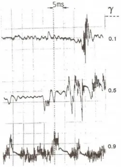
(with respect to γ) to the similarly unfiltered hot-wire signal traces of Figure 2-6 by Fasihfar and Johnson (1992). Figure 2-7 also provides a demonstration of how the filtered near wall hot-wire velocity profiles vary with increasing streamwise displacement (and therefore intermittency). Please note that these signals have been arbitrarily offset (by their integer count index * 5 m/s, where the filtered signals have been amplified by a factor of 3) such that they are stratified, rather than overlaid, for the sake of clarity. Additionally the quoted intermittency values in the plot legend are representative of the intermittencies experienced over the entire flow signal (of 30 seconds) but, again for the sake of clarity, only a small portion of the signal (the first 1 second) is shown such that discrete bursts are clearly visible.

Furthermore, each of the signal traces in the aforementioned demonstrative figure have been produced at a fixed height with each boundary layer rather than at self-similar non-dimensional wall normal displacements, with respect to the boundary layer thickness.

17

Figure 2-6 - Unfiltered hot-wire signal traces Fasihfar and Johnson (1992)

18

Figure 2-8 - Filtered velocity for intermittent signal (Fasihfar and Johnson (1992))

In addition to the advent of turbulent bursts for signals with non-zero intermittency, one can also observe from Figure 2-7 that the burst frequency (as in the rate at which bursts occur as opposed to frequencies associated with the burst structures themselves) increases with Reynolds number until the flow signal is effectively saturated with turbulent bursts at 100% intermittency – the end of transition.

2.3.2 Influence of Freestream Turbulence on Transition – Intensity and Length Scale

In the past many researchers, such as Hall and Gibbings (1972) and Abu-Ghannam and Shaw (1980), have investigated the effects of freestream turbulence intensity on the onset and propagation of transition in flat plate two dimensional boundary layers. They have typically produced empirical transition correlations which predict the momentum thickness Reynolds numbers for the start and end of transition based on the freestream turbulence intensity.

19

preliminary design because transition is an extremely complex phenomenon and is highly dependent on the environment in which the tests were conducted. As such results can differ markedly from one testing environment to another and replicating the results of others is not something which is readily achievable. This is further compounded, particularly for low turbulence intensity

environments, by the effects of surface roughness in that no two plates or wings have identical roughness profiles and, as such, results for the same specification can be significantly different if, that is, the surfaces are not hydraulically smooth, albeit this is usually the case if so desired.

Jonáš et al. (2000) point out that when it comes to turbulence intensity and length scales it is the former which has benefited from the greatest degree of attention, in terms of the research undertaken, but there are reasons to expect that length scale imposes a significant influence also. This largely stems from the fact that the larger the length scale of the freestream turbulence, the lesser the dissipation/decay, with the opposite holding true. As a consequence the boundary layer is perturbed in a different manner downstream even if two initially dissimilar flows happen to match at the leading edge. Correlations do exist which characterise the flow in terms of both turbulence intensity and length scale and these have been applied with some success, see Jonáš et al. (2000).

2.3.3 Influence of Pressure Gradient on Transition

The effect of pressure gradient on the evolution of the transition process is very much dependent on the flow configuration itself. The significance of pressure gradients is most often taught within the context of incompressible 2-D boundary layer theory. That is typically to say that a positive pressure gradient in the streamwise direction will have an adverse effect on stability and, similarly, a negative pressure gradient conforms to favourable conditions, enhancing stability.

20

( ) Equation 2-10

If one considers a 2-D flow then is zero and since (for a flat surface, where u = 0) then

can be neglected, thus leaving Equation 2-11 as expressing the pressure gradient;

( ) Equation 2-11

Henceforth it is understood that the pressure gradient, both in its magnitude and polarity, will go a long way towards determining the shape of the velocity profile in the near wall region of a flat plate laminar boundary layer. For a negative pressure gradient causing the flow to accelerate in the streamwise direction, , must also be negative and this negative magnitude actually persists until . A negative pressure gradient has the effect of filling out the velocity profiles, due to the increased curvature, and hence the boundary layer thickness, displacement thickness and momentum thickness will be reduced for the trade-off that the shear stress on the fluid will be higher in the near wall region owing to the increased velocity gradients. All of which conspire to increase the stability of the boundary layers under the influence of such pressure gradients, hence in 2-D flows these are often termed favourable pressure gradients.

21

reduced stability and accelerate the transition process. As such positive streamwise pressure gradients in 2-D boundary layers are termed as being adverse pressure gradients. Should such an adverse pressure gradient be of sufficient severity, or persist for sufficient spatial duration, it is likely that separation would be instigated. Separation of the mean flow occurs when the shear stress, and therefore the wall normal velocity gradient, drops to 0.

The severity of adverse pressure gradient which a boundary layer can sustain without separation also depends on the nature (laminar, turbulent or indeed transitional) of the boundary layer itself. Turbulent boundary layers are known to be less susceptible to the effects of adverse pressure gradients owing to the enhanced mixing associated with turbulence which act to suppress

separation by producing a continuous flux of momentum towards the wall which effectively keeps the boundary layer energised and therefore attached.

This is perhaps best illustrated with the practical example of dimples on a golf ball where the Reynolds numbers are sufficiently high that separation occurs. The dimples act to turbulate the flow, maintaining flow attachment for longer, relative to the smooth, laminar counterpart of a perfect sphere and thus keeping pressure drag to a minimum by increasing the separation to approximately 130° from 80° in the laminar case and therefore minimising the size of the wake. Note that the separation angles quoted here are merely demonstrative figures and, in reality, the actual separation angles will vary depending on Reynolds number and the background environment.

22

2.4

Boundary Layer Theory

The following section provides a brief overview of the theoretical frameworks for which boundary layer theory has developed from, in strict relation to laminar, transitional and turbulent boundary layer flows. These are initially considered from the classical 2-D unswept viewpoint, whereafter (in section 2.5) the focus shifts towards 3-D boundary layers and Falkner-Skan-Cooke mean velocity profiles which are closely correlated to the flow fields which were present in the experimental and numerical work presented in Chapter 4 and Chapter 5.

2.4.1 Laminar Boundary Layers

In laminar flows the fluid particles tend to move in parallel layers (laminae) but in the boundary layer each laminate layer propagates at different relative velocities as the motion is restricted by the action of shear stress, initiated by the lack of slip (usually no slip) at the solid boundary.

For all flows considered in this thesis there are two (classical) physical conservation arguments which are abided by. These being; firstly that mass is conserved and secondly momentum is conserved.

The continuity equation, in three-dimensional Cartesian notation, for steady incompressible flow, where source terms and body forces due to gravity can be ignored (where air is considered to be the fluid medium) is as follows in Equation 2-12.

Equation 2-12

23

Equation 2-13

Likewise the momentum equations are;

( )

( ) Equation 2-14

( )

( ) Equation 2-15

( )

( ) Equation 2-16

again, in vector notation;

( ) Equation 2-17

Note that, subject to the inclusion of the transient term; , the above equations are those which are solved for direct numerical simulations (DNS) in incompressible flows, in that no modelling of the fluctuating terms is used for solution time brevity, at the expense of accuracy/physicality.

2.4.2 Transitional Boundary Layers

24

This approach involves quantifying the positions, with respect to the streamwise displacements from the leading edge and their respective target intermittencies for unskewed boundary layer profiles. The following streamwise positions can then be trapped through linear interpolation of the near wall data points; at 1%, 25%, 75% and 99% intermittency. 1% is considered to be where the transition starts and 99% where transition is completed and the difference between these two parameters represents the streamwise displacement over which the transition takes place – i.e. the transition length.

Dhawan and Narasimha (1958) then postulated the following relationship (Equation 2-19) for the distribution of intermittency with respect to a flat plate zero pressure gradient boundary layer in the near wall region, where Equation 2-18 provides the definition of the arbitrary λ parameter.

Equation 2-18

( ) ( ( ) ) Equation 2-19

Thereafter transitional boundary layer parameters can be approximated as an intermittency

weighted average of laminar and turbulent profiles, as suggested by Emmons (1951), for example for the skin friction coefficient where L and T denote laminar and turbulent portions;

( ) Equation 2-20

25

empirical correlation of Abu-Ghannam and Shaw (1980) – Equation 2-21 to predict the start of transition.

( ) Equation 2-21

Unfortunately, the computational effort required to directly solve the Navier-Stokes equations at relevant Reynolds numbers using DNS is large and so the use of empirically based RANS methods are more commonplace. Such approaches are perhaps valid (and have certainly proven to be successful commercially) and to a limited extent physically realistic, where one does not deviate significantly from simple test cases (for example the T3 ERCOFTAC test cases zero pressure gradient test cases from Savill (1992) as in Steelant and Dick (1996)) but reliable, robust general transition models which span a wide variety of problems don’t exist, as of yet.

In Johnson (2002) a method of predicting transition without empiricism or DNS is presented by studying the receptivity of Poulhausen boundary layer profiles to various vortex orientations. This was subsequently improved to similar studies on developing laminar boundary layer profiles in Johnson (2011a). One of the objectives of the current thesis is to extend this to non-zero pressure gradients and swept flows.

2.4.3 Turbulent Boundary Layers

26

expressed all properties as the sum of mean and fluctuating components, therefore, in the case of incompressible, isothermal flows, forming the time-averaged continuity and Navier stokes

equations. Furthermore, since virtually all engineering problems involve inhomogeneous turbulence, time-averaging represents the most appropriate form of Reynolds averaging (Wilcox (1998)). There are several statistical averaging choices available, but given that hot-wire

measurements are frequently recorded with single component hot-wires resolving the Reynolds stresses is not something which can be achieved from single wire data. This is clear with the following explanation of the Reynolds-averaged Navier-Stokes equations (RANS) in the case of spatially stationary turbulence.

To start with we formally express the instantaneous velocity, ( ), of such a flow as;

( ) ( ) ( ) Equation 2-22

This is to say that the instantaneous velocity is the sum of the mean and the fluctuating component where the mean is time-averaged, as in Equation 2-23;

( )

∫ ( )

Equation 2-23

27

The time-average of the fluctuating component, on the other hand, is zero, owing to the mean and time-average of the mean being equivalent. However, there is no a priori reason for the product of different fluctuating properties to be zero, such as is in turbulent flows where ‘apparent stresses’ – i.e. the Reynolds stresses, are observed (Wilcox (1998)).

For the reader interested in studying turbulent flows the book by Tennekes and Lumley (1972) offers insight into most of the salient macroscopic features of such flows which are listed below;

Irregularity - Turbulent flows are irregular and chaotic. They are the product of a broad spectrum of different eddy-sizes/length scales. It is however, contrary to popular misconceptions, deterministic and fully described by the Navier-Stokes equations. That is to say for two separate ‘numerical experiments’ with the same set of input conditions that identical results will be produced. However, the background acoustic noise that one may observe during physical experimentation may, on the other hand, essentially be random. In order to sufficiently resolve such issues a valid DNS approach may have to include the full wind tunnel and possibly the laboratory environment itself in the calculation, which would of course be exceptionally (and prohibitively) expensive. As such many of the inflow boundary conditions on numerical simulations, which solve some form of the Navier-Stokes equations, utilise random algorithms to superimpose turbulent structures on the incoming mean flow to represent freestream turbulence, see the synthetic-eddy-method of Jarrin et al. (2006) for example. Theoretically, with a well-designed synthetic inflow boundary condition, which is representative of the complementary experimental set-up, it would be possible to obtain convergence with the statistically steady mean properties. This would hold true if the Reynolds averaged results for solution time tending towards infinity and, likewise, an infinite number of ensemble averaged experiments/Reynolds averaged experiments over infinite sampling time.

28

pressure losses due to increased ‘blockage’. Furthermore, owing to the enhanced diffusivity, the fluid stress can be several orders of magnitude greater than that of a corresponding laminar flow field.

Three-dimensionality - Turbulent flows are inherently three-dimensional, as discussed previously in chapter 1 and in Versteeg and Malalasekera (2007).

Dissipation - Turbulent flows dissipate their energy through a cascade process. The largest eddies, operating at the integral length scale, which are on the order of the flow geometry (e.g. mesh spacing size), extract their kinetic energy from the freestream. Smaller eddies consume their energy from the larger eddies, and the kinetic energy of the smallest eddies (operating at the Kolmogorov lengthscale) are dissipated as heat/internal energy through the action of molecular viscosity. This process of energy transferral, from the largest to the smallest eddies, is called the cascade process. Continuum – The smallest turbulent eddies are typically much larger than the molecular scale and, hence, classical continuum assumptions, analogous to those in classical mechanics, are applicable. That is to say for turbulent flows, in the case of numerical simulations, there is no necessity to model discrete particle collisions although there are methods which model the particle collisions, such as Lattice-Boltzmann methods.

29

( ) Equation 2-24

where the empirical coefficient 2.44 is the reciprocal of von Karman’s constant κ of 0.41, attributed to Von Karman (1930) and the latter coefficient (often termed the ‘additive constant’ as in Marusic et al. (2010)) of 4.9 (or C+) is typical of those expressed for smooth walls, e.g. in Schlichting and Gersten (2000) the value 5.0 is quoted. Furthermore u+ and y+ are defined as follows, with uτ, also known as the friction velocity, given in Equation 2-27;

Equation 2-25

Equation 2-26

where; √ Equation 2-27

The law of the wall (in the form of Equation 2-24) effectively states that the mean velocity in the form of u+ in a turbulent flow is proportional to the natural logarithmic distance from the boundary within a certain range of y+ values. The empirical law is generally found to be applicable for y+ values greater than 70, Schlichting and Gersten (2000), although some sources observe collapse in their data down to y+ of 30, e.g. Kline et al. (1967).

Beneath the law of the wall region resides the viscous sublayer, with a buffer layer in between. In Schlichting and Gersten (2000) the viscous sublayer is said to exist for y+ values below 5, with the buffer layer spanning the gap to the log law region. In the viscous sublayer the u+ and y+ values are observed to be equal in magnitude, i.e;

30

However, in the buffer layer Equation 2-24 and Equation 2-25 are not applicable. Nevertheless the buffer layer is still considered as part of the near wall region, which was defined as being by Cantwell (1981) within which region the majority of turbulent energy production is contained so it is therefore not to be considered an insignificant region.

2.5

3-D Boundary Layers

There are many forms of classical 3-D (including axisymmetrical) boundary layers, as in boundary layers where the direction of the mean flow forms a function of the normal coordinate, Schmid and Henningson (2001), which have been the subject of several high quality research studies. The majority of these classical problems are discussed in Schlichting’s Boundary Layer Theory (Schlichting (1968)) and include the boundary layers on yawed cylinders, rotating disks, cones, spheres,

ellipsoids, various combinations of geometrical intersections (‘interference drag’) and of course flat plates, with and without sweep. Gregory et al. (1955) were able to arrive at the conclusion that the flow over a rotating disk is similar to that of swept wing flow, given that the crossflow vortices are corotating in both cases.

31

(2012), such as rotating discs (see Gregory et al. (1955)), rotating cones (see Kobayashi et al. (1983)) and swept cylinders (see Poll (1985)).

Similarly, two such well-studied flow configurations are boundary layers over swept wings and internally within turbomachinery, as previously discussed. Such cases are well described by a family of solutions to the boundary layer equations known as the Falkner-Skan-Cooke similarity solutions Kurian et al. (2011). These solutions are stable to the development of Tollmien-Schlichting waves but are sensitive to, and often governed by, crossflow instabilities Kurian et al. (2011). Crossflow instabilities exist as stationary or travelling waves and the transition process, where all other instability mechanisms (such as centrifugal and TS) remain sub-critical, will be governed by either waveform mode Kurian et al. (2011). Typically more effort is spent trying to replicate circumstances where stationary crossflow modes (as opposed to travelling) are deemed responsible for the

transition process as this is the scenario most often seen in free-flight conditions Kurian et al. (2011) on aircraft.

In order for this to be achieved there is a drive towards minimising freestream turbulence levels in wind tunnels. For instance at the MTL (Minimum Turbulence Level or Mårten Theodore Landahl, named after its late creator Lindgren and Johansson (2002b)) facility at KTH – Royal Institute of Technology in Sweden the streamwise freestream turbulence intensity is quoted as less than 0.025% (when high-pass filtered) at 35m/s in Lindgren and Johansson (2002b). It is interesting to note that similar readings were observed at the MTL facility a decade previously in Johansson (1992). Ideally (from their perspective) these turbulence intensities would tend towards 0% which would allow something of a replication of quiescent atmospheric conditions, in the relative frame of reference moving at the freestream velocity, similar to that experienced in free-flight. In Kachanov (2000a) it is stated that the main problem with all such low-turbulence facilities is that they don’t actually

32

of freestream turbulence are susceptible to errors caused by vibration. Thereafter changes in the freestream turbulence intensities, and often other important parameters such as turbulent length scale etc., can be successfully modulated through judicious choice and installation of turbulent generating grids upstream of the test section. Similarly, several experiments have been performed in water towing tank facilities, such as in Bippes (1990) – on cylinders in this case, following a similar rationale regarding freestream turbulence intensity.

Although crossflow instability has been studied extensively it is still not well described by the

method Kurian et al. (2011), which has been used successfully with 2-D boundary layer flows, see for example Arnal (1994) and other work on the parabolised stability equations (PSE) such as Herbert (1997). As with 2-D boundary layers, reliable prediction of the transition process is dependent upon detailed knowledge of the disturbance environment and, hence, accurate predictions require an understanding of the receptivity process (Kurian et al. (2011)). As such this is the area in which the efforts exerted for the current work have been channelled towards, both in terms of the

experimental and numerical receptivity work.

33

are blessed with the best resources are limited to Reynolds numbers which typically aren’t

comparable with what would be observed in ‘real-world’ scenarios. In general terms one can now reach realistic Reynolds numbers for bypass, albeit not for natural transition. For example Johnson (2013) performed a DNS on a flat plate boundary layer for Reθ = 2240 using a a grid with up to 140 million grid points, solving through a spectral method whilst utilising a periodic boundary condition in the streamwise direction. Such approximations are effectively necessary owing to the (present) prohibitively expensive nature of the process and, as with most modelling, each present their own numerical artefacts.

2.5.1 Falkner-Skan-Cooke Boundary Layer Example

Mathematically speaking, an approximation of the velocity profiles in swept three-dimensional boundary layers are successfully provided by the Falkner-Skan-Cooke similarity solutions derived by Cooke (1950). These similarity solutions effectively extend the von Karman-Pohlhausen method Pohlhausen (1921) to another dimension Cooke (1950) using the Falkner-Skan third order ordinary differential equation (ODE) for wedge flows attributed to Falkner and Skan (1931) as a starting point. The Falkner-Skan-Cooke boundary layer is frequently used as the base for swept wing analyses since it comprises both a pressure gradient and sweep angle, Tempelmann et al. (2010). Three

dimensional laminar boundary layers on swept wings with a pressure gradient are well described by these Falkner-Skan-Cooke similarity solutions to the boundary layer equations (Kurian et al. (2011)). Please note that the Falkner-Skan-Cooke general solutions can be reduced back to the special case of Blasius flow in the absence of crossflow and pressure gradient - Chevalier et al. (2007).

34

( ) Equation 2-29

where;

Equation 2-30

therefore;

Equation 2-31

The non-dimensional boundary layer thickness is also given by the similarity variable η as;

√( ) ( )

Equation 2-32

and when ; and , i.e tending towards potential flow outside of the boundary layer.

Using the stream function approach to implicitly solve continuity gives a stream function, ψ, of the following form;

( ) √(

) ( ) Equation 2-33

eventually yielding the following differential equations for Falkner-Skan-Cooke flow;

_{( ) Equation 2-34}

_{Equation 2-35}

35

The effects of the βH parameter (in Equation 2-34) on the Falkner-Skan equation were investigated by Hartree (1937) who found that physical solutions, using a shooting method approach, were viable for the range;

This was because values of m greater than unity resulted in floating point errors and, on the other periphery, too low a value of m will physically instigate flow separation. Stewartson (1954)

suggested that the Falkner-Skan equation can be thought of (qualitatively) as analogous to non-zero pressure gradient flows where the pressure gradient is prescribed by the βH parameter, hence the corresponding separation which occurs when the m (or βH) parameters are too severe and, by analogy, so too would be the pressure gradient.

The second of the two ODE’s (Equation 2-35) and, in essence, the contribution of Cooke (1950) utilises the previous solution for f in the Falkner-Skan equation and, once solved, allows for computation of the streamwise and crossflow velocities as follows;

( ) Equation 2-36

( ) ( ) Equation 2-37

where θ is relative to the leading edge and;

( ) _{Equation 2-38}

36

√( ) ( )

∫ ( ) Equation 2-39

The Falkner-Skan-Cooke equations can’t be solved analytically and, as such, approximate numerical methods are utilised to obtain solutions, in conjunction with the following boundary conditions for this boundary value problem;

( ) ( )

( )

( )

( )

The results of Stemmer (2010) are presented here for Falkner-Skan-Cooke profiles at two different βH values, -0.1 and 1.0, in Figure 2-9. These results are later replicated in section 4.2.4.

37

2.5.2 Instability Mechanisms for Swept Transition

There are four fundamental instability modes present on a swept (wing) laminar boundary layer flow and these comprise; attachment line, streamwise (Tollmien Schlichting), crossflow and centrifugal instabilities, Dagenhart and Saric (1999), and these are depicted in Figure 2-10, relative to their principal area of action. When dealing with flat plates, centrifugal instability, which can lead to the production of Görtler vortices in concave regions of wings, does not feature and, therefore, is afforded no additional consideration here.

Figure 2-10 - Possible instability mechanisms acting on a swept wing and their prevalent locations (Bippes (1999))

38

In Uranga et al. (2011) the parameters which are stated to be important in crossflow stability studies are the height of the inflection point, the velocity gradient at this point and the maximum crossflow velocity. An example of a critical Reynolds number for crossflow instability is given in Zurigat and Malik (1995) as Equation 2-40.

̅ Equation 2-40

where ̅ is the magnitude of the maximum crossflow velocity and is the boundary layer

thickness, within which the crossflow velocity is less than 10% of ̅ . Other forms of critical Recf exist and can even be compared with similar criteria for Tollmien-Schlichting natural transition, to

estimate the extent and influence of the respective regions for a given scenario.

The baseflow of attachment line instability is a swept Hiemenz flow, that is to say a stagnation flow with a superimposed crossflow/spanwise component (Gad-el-Hak and Tsai (2005)). Attachment-line instability is a linear viscous instability, Gad-el-Hak and Tsai (2005), whereas crossflow instabilities (whilst similarly linear) are of the inviscid type. As a consquence, passive suction methods (on which significant work has been conducted along with other transition control methodologies) for

controlling transition in swept wing flows are less effective where crossflow instability dominates, owing to crossflow instabilities being inflectional in nature. This is in contrast to Tollmien-Schlichting instabilities, which are more conducive to such control, given their viscous instability nature (Reed and Saric (1989)).

39

Downstream of the crossflow instability region at the leading edge streamwise instability (basically Tollmien Schlichting activity) tends to dominate swept natural transition processes, as depicted in Figure 2-11. In Saric and Yeates (1985) it is stated that for the mid-chord region of a swept wing the stability is governed by Tollmien-Schlichting waves, but this would only be applicable in cases where the freestream turbulence intensity is lower than that for bypass transition to take place, as is typically the case in free flight conditions.

In swept-wing boundary layers Tollmien-Schlichting instability waves can also play a significant role in the process of transition (Kachanov (2000a)). However, the most important mechanism

responsible for natural 3-D transition is associated with the crossflow instability (Kachanov (2000a)). Similar to swept wings, swept flat plate boundary layers are also known to exhibit strongly

inflectional (crossflow) instabilities (Tempelmann (2011)).

The reason why crossflow instability dominates towards the leading edge in (swept) natural transition is because the Tollmien Schlichting activity is attenuated by the initially favourable pressure gradient and, generally speaking, crossflow instability is the dominant instability

40

Figure 2-11 - Crossflow and Tollmien Schlichting instability waves on a swept wing - Oertel (2010)

41

However, with significantly increased freestream turbulence intensity these primary instability modes will largely by bypassed and the transition will take place through a bypass mechanism. For a boundary layer transitioning through a bypass mechanism the flow is characterised by the growth of high and low speed streaks which are generated through what’s known as the Klebanoff mode (Kendall (1985)). These streaks are also observed in the near wall region of fully turbulent flow.

In Brandt (2003) it is stated that streaks are seen to appear with boundary layers that are subject to significantly high free-stream turbulence levels, as such attention is now drawn to streaky structures and Klebanoff modes. Klebanoff modes appear to be caused by freestream turbulence and take the form of streamwise streaks (Kudar et al. (2006)). Klebanoff modes are fundamentally different to TS instability modes in that the former grows algebraically, as opposed to the latter which grow in an exponential fashion (Kudar et al. (2006)). Klebanoff modes are, therefore, not wavelike in form.

It was observed by Gray (1952) (in both real flight and wind tunnel conditions on swept wings - Kohama (1987)) that regularly-aligned streaks appear almost along the outer streamline of the boundary layer. These flow patterns are also observed in non-zero pressure gradients on swept flat plates, as in Saric and Yeates (1985). It is thought that these streaks are caused via the action of co-rotating stationary vortices (Kohama (1987)) and, as such, are perhaps limited to cases where the freestream turbulence intensity is below the order of magnitude where the vortices become unsteady

Kudar et al. (2006) presented a study of Klebanoff modes, in the context of 3-D transition, through a simplified DNS study, with the high values of turbulence intensity approximated through a fictitious body force, using the aforementioned Falkner-Skan-Cooke family of velocity profiles as their

42

al. (2004), have artificially generated similar streaks using spanwise arrays of cylindrical roughness elements.

2.5.3 Receptivity in 3-D Boundary Layers

Receptivity as a term, if not a concept, was first coined in Morkovin (1969) and represents the first stage of the transition process Jahanmiri (2011) – see Figure 2-2. It is first of all important to understand that no flow in nature, or indeed in engineering applications, is free from disturbances Jahanmiri (2011) and that true transition prediction is dependent upon understanding/quantifying the disturbance environment and receptivity processes which trigger disturbances inside the boundary layer that subsequently grow Kurian et al. (2011).

The receptivity process, or mechanism, is that in which disturbances in the freestream enter, and have the effect of, exciting instability waves inside wall-bounded and free-shear layers (Kerschen (1993)). It is known that the nature of the stability of these respective layers (free vs. bounded) are fundamentally different (Saric et al. (2002)). In Kerschen (1993) receptivity is sub-divided into two categories – that of natural and forced receptivity. In natural receptivity the aforementioned waves are excited by acoustic and vortical disturbances which, as the name suggests, appear naturally in freestream flows.

43

application of surface non-uniformities, as per the theoretical studies of Fyodorov (1988) (in Russian) Kachanov (2000b) and the respective experimental studies and comparisons thereafter such as Ivanov and Kachanov (1994) and Crouch et al. (1997), or by introducing spanwise non-uniformity of the potential flow.

Since these freestream disturbances take the form of vorticity, sound, vibrations or surface

roughness, the influences are incompletely understood (Saric et al. (2002)). What is known however is that these disturbances can penetrate into the boundary layer via its respective boundaries Jahanmiri (2011), such as the horizon of the boundary layer thickness, at the boundary layer origin (such as the leading edge of a wing - Kachanov (2000a)) or the surface itself, such as a flat plate. Some combined methods of the above are also possible (Kachanov (2000a)).