Doctoral Thesis
Estimating the distribution of the mass
component of sea level trends using tide
gauges, altimetry and steric
reconstructions.
Author:
Clare
Bellingham
Supervisors:
Prof. Ric
Williams
Prof. Chris
Hughes
Dr. Simon
Holgate
Examiners:
Prof. Philip
Woodworth
Prof. Mikis
Tsimplis
A thesis submitted in fulfilment of the requirements
for the degree of Doctor of Philosophy
in the
Department of Earth, Ocean and Ecological Sciences SCHOOL OF ENVIRONMENTAL SCIENCES
I, ClareBellingham, declare that this thesis titled, ’Estimating the distribution
of the mass component of sea level trends using tide gauges, altimetry and steric reconstructions.’ and the work presented in it are my own. I confirm that:
∎ This work was done wholly or mainly while in candidature for a research
degree at this University.
∎ Where any part of this thesis has previously been submitted for a degree or
any other qualification at this University or any other institution, this has been clearly stated.
∎ Where I have consulted the published work of others, this is always clearly
attributed.
∎ Where I have quoted from the work of others, the source is always given.
With the exception of such quotations, this thesis is entirely my own work.
∎ I have acknowledged all main sources of help.
∎ Where the thesis is based on work done by myself jointly with others, I have
made clear exactly what was done by others and what I have contributed myself.
Signed: Clare Bellingham
Date: 10th June 2015
most of the life on Earth. 97% of Earth’s water is there. It’s the blue heart of the
planet - we should take care of our heart. It’s what makes life possible for us. We
still have a really good chance to make things better than they are. They won’t get
better unless we take the action and inspire others to do the same thing. No one
is without power. Everybody has the capacity to do something.”
Abstract
Department of Earth, Ocean and Ecological Sciences SCHOOL OF ENVIRONMENTAL SCIENCES
Doctor of Philosophy
Estimating the distribution of the mass component of sea level trends using tide gauges, altimetry and steric reconstructions.
by Clare Bellingham
This thesis is written with full acknowledgement of the contributions, discussions and insight from my supervisors Ric Williams, Chris Hughes and Simon Holgate. Additional discussions from Mark Tamisiea concerning the fingerprints, Svetlana Jevrejeva concerning tide gauges and land corrections and Simon Williams con-cerning the annealing code were invaluable.
Thanks to the University of Liverpool and the National Oceanography Centre Liverpool for offering me this valuable and rewarding experience.
With thanks for initial discussions and the use of the Smith et al. (2007) data set from Doug Smith and to everyone at PSMSL for help with using tide gauge data.
Thanks to the University of Hawai’i at M˜anoa, especially to Mark Merrifield and Phil Thompson for inspiring talks and useful comments towards this thesis.
Grateful acknowledgements to NERC for funding this PhD and to the University of Liverpool John Lennon Memorial Scholarship for the award to help with my childcare.
Special thanks to my children Leon, Jessie, Kara and Elliot for the inspiration to keep learning, and to friends and family who make it all worth while.
Declaration of Authorship i
Abstract iii
Acknowledgements iv
Contents v
List of Figures ix
List of Tables xiv
Abbreviations xvi
Symbols xviii
1 Background of Sea Level Trends 1
1.1 Paleo sea level . . . 3
1.2 Salt marsh and long tide gauges . . . 4
1.3 The global mean sea level time series . . . 4
1.4 The steric contribution . . . 5
1.5 Global sea level budget . . . 6
1.6 Altimetric measurements . . . 8
1.7 Mass changes . . . 9
1.8 Large scale variability . . . 11
1.9 Acceleration in sea level. . . 12
1.10 The use of zonal averages . . . 13
2 Theoretical Background 14 2.1 Introduction . . . 14
2.1.1 Mean sea level . . . 16
2.1.2 Geoid and definitions . . . 16
2.1.3 Basic definitions . . . 17
2.1.4 Absolute and Relative Sea Level . . . 17
2.1.5 Steric and mass components. . . 18
2.1.6 Gravitational corrections . . . 19
2.1.7 Crustal Motion. . . 20
2.2 Augmented Dynamic Topography . . . 20
2.3 Applying observing systems . . . 22
2.3.1 V LD correction to tide gauges using altimetry. . . 23
2.3.2 V LDcorrection to tide gauges using the Global Positioning System (GPS). . . 23
2.3.3 GIA only correction to tide gauges and altimetry . . . 24
2.4 Barystatic Sea Level . . . 24
2.5 Summary . . . 26
3 Tide Gauge Trends in Sea Level and the Effects of Different Sub-sets 27 3.1 Introduction . . . 28
3.1.1 Regional trends . . . 29
3.2 Tide gauge data . . . 30
3.2.1 Calculating tide gauge trends . . . 33
3.3 Choosing a subset . . . 34
3.3.1 All tide gauges . . . 35
3.3.2 Long time series gauges . . . 37
3.3.3 Uniform spatial coverage gauges . . . 38
3.3.4 500 gauges . . . 39
3.3.5 Data analysis. . . 40
3.4 V LD and G changes. . . 42
3.4.1 Converting ASL toτ . . . 42
3.4.2 Correcting ASL forGIA effects . . . 46
3.4.3 Mass redistribution model - Relative solutions for GIA. . . . 46
3.4.4 Altimetry at tide gauges . . . 48
3.4.5 Global Positioning System . . . 49
3.5 Comparing corrected tide gauge trends. . . 52
3.6 The global average from tide gauges . . . 54
3.7 Trends 1993 to 2010 as a function of latitude . . . 57
3.8 Discussion . . . 61
3.9 Summary . . . 63
4 Steric Height Trends in Sea Level 65 4.1 The steric height component of sea level . . . 65
4.2 Background . . . 67
4.3 Data . . . 71
4.3.1 The Smith and Murphy (2007) dataset . . . 72
4.3.2 The Ingleby and Huddleston (2007) dataset . . . 73
4.3.3 The Ishii and Kimoto (2009) dataset. . . 75
4.3.4 The Levitus et al. (2009) dataset . . . 76
4.3.5 The Carton et al. (2000) dataset . . . 76
4.4 The thermodynamic equation for sea water TEOS-10 . . . 77
4.4.1 Absolute Salinity and Practical Salinity . . . 78
4.4.2 Conservative and Potential Temperature . . . 79
4.5 Comparing the 5 data sets . . . 81
4.6 The global-average trend in steric height. . . 83
4.7 Zonal average of steric trends . . . 86
4.7.1 Zonal averages for different time periods for each data set . . 88
4.7.2 The relevance of the reference depth . . . 91
4.8 Summary . . . 94
5 Sea Level Trends from Altimeter Measurements 96 5.1 Absolute sea level . . . 97
5.2 Some background. . . 100
5.3 Data . . . 100
5.3.1 The global mean dynamic topography . . . 102
5.4 The global trend . . . 103
5.4.1 Inland Seas . . . 103
5.5 GIA corrections to the altimetry data . . . 104
5.6 Altimetry at tide gauges . . . 107
5.7 Reference frames . . . 110
5.8 Discussion . . . 110
5.9 Summary . . . 116
6 Calculation of the Implied Mass Component of Sea Level Trends118 6.1 Introduction . . . 119
6.1.1 Land exchange . . . 119
6.1.2 Exchange with the cryosphere. . . 120
6.1.3 Ice sheets . . . 121
6.1.4 Glaciers . . . 122
6.1.5 Measuring the mass component . . . 123
6.2 The implied mass. . . 124
6.3 Fingerprints . . . 126
6.4 Expectation of fingerprint response using IPCC AR5 values . . . 129
6.5 Comparing total and steric sea level . . . 130
6.5.1 Mass trends from tide gauges . . . 131
6.5.2 Mass trends from altimetry . . . 132
6.5.3 Mass derived from full depth steric only. . . 133
6.6 Solving for the melt rate coefficients . . . 134
6.7 Coefficient results . . . 137
6.7.1 Assessing the robustness of the analysis . . . 143
6.8 Weighting the results . . . 144
6.9 Weighted coefficient results . . . 147
6.10 Redefining the errors on rates from tide gauges and altimetry using
weights . . . 149
6.11 Discussion . . . 152
6.12 Summary . . . 157
7 Discussion and analysis 163 7.1 Basin scale distributions . . . 168
7.1.1 East and West contrasts . . . 169
7.2 Changes in rates . . . 169
7.3 Mass trends from each steric reconstruction . . . 173
7.4 Mass redistribution compared to higher recent rates . . . 177
7.5 Future development . . . 179
A Coefficients from all tide gauges 181
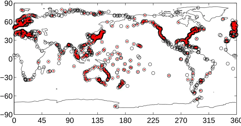
3.1 Map showing locations of all tide gauges in the PSMSL database
and those with data during 1993 - 2010 . . . 31
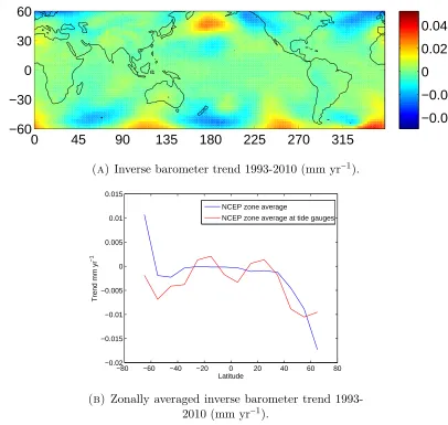
3.2 Map of the inverse barometer correction for 1993-2010 calculated
us-ing equation 3.1 usus-ing data downloaded from NCEP (figure (3.2a)). Shown also as zonal averages (figure (3.2b)) both at all grid points
(blue) and at tide gauge locations (red). . . 32
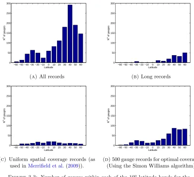
3.3 Number of gauges within each of the 10o latitude bands for the four
subsets of tide gauges . . . 35
3.4 Location of tide gauge stations for the four subsets of tide gauge
records.. . . 36
3.5 Relative sea level height (mm) measured by tide gauges as a function
of latitude.. . . 37
3.6 The convex hull shows the volume of Earth represented with 500
tide gauges. . . 40
3.7 Time series (1955-2010) of tide gauge 18 year running trends (mm
yr−1) within latitude bands . . . 43
3.8 Histograms showing tide gauge trends from all tide gauges with
trends from 1993 - 2010 for each latitude band.. . . 44
3.9 GIA contribution to rate of change of (G′
+V LD). . . 47
3.10 V LDvalues added to each tide gauge as a correction forGIAusing
the mass redistribution model, ICE-5G (Peltier, 2004) (mm yr−1). . 47
3.11 Miyake Sima time series (mm). . . 49
3.12 Tide gauge locations showing the difference in trend for 1993 to
2010 between altimetry and tide gauges. . . 50
3.13 Location of tide gauges and GPS sites, showing their distances apart. 51
3.14 Location of tide gauges and GPS sites, showing tide gauges over
500km and 1000km from the nearest GPS site. . . 52
3.15 Values of V LD at GPS corrected tide gauge stations (mm yr−1) . . 53
3.16 All uncorrected PSMSL RLR tide gauges rates for the period 1993
to 2010 (mm yr−1) . . . 54
3.17 All tide gauges corrected for V LD and (G′+V LD) showing sea
level trends for 1993 to 2010. . . 55
3.18 The global trend for sea level using all tide gauges . . . 56
3.19 Trend as in 3.18a but for all gauges only in the Northern Hemisphere
between latitudes 20oN to 60oN (mm yr−1) . . . 56
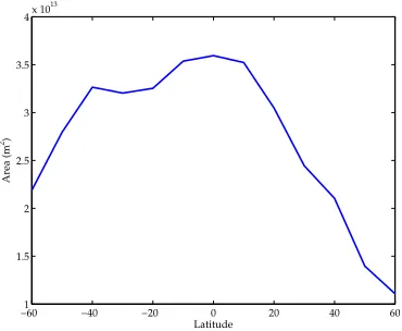
3.20 Area of ocean within each latitude band (m2). . . 58
3.21 Zonal averages of 1993 to 2010 trends in sea level for 4 tide gauge
selections showing 3 separate corrections for V LD. . . 59
3.22 Area weighted zonal averages of 1993 to 2010 trends in sea level. . . 60
4.1 Annual mean steric height (m), with the global annual mean
re-moved (Ishii and Kimoto, 2009) for the year 2009. . . 67
4.2 Observational subsurface temperature profile sampling comparing
January 1958 with January 2010 . . . 69
4.3 Absolute Salinity minus Practical Salinity cross sections of the
In-dian, Pacific and Atlantic and Southern Oceans (g kg−1) during 2008 80
4.4 Conservative Temperature mean depth profiles for 2008 (oC)
(In-gleby and Huddleston, 2007) . . . 81
4.5 Conservative Temperature minus Potential Temperature cross
sec-tions of the Pacific and Atlantic Oceans (oC) during 2008. . . . 82
4.6 Atlantic, Pacific and Indian Ocean comparison of 5 temperature
data sets using the 14o C isotherm anomaly, relative to the long
term average depth. . . 84
4.7 Latitudinal average of steric height anomaly (m) . . . 85
4.8 Time series of the area weighted global average steric mean trend
calculated as 18 year running linear trends centred on the middle
year for 5 data sets (mm yr−1). . . . 87
4.9 Steric trends between 1993 and 2010 (mm yr−1) for 5 data sets. . . . 88
4.10 Mean zonal trends of 5 steric reconstructions for 3 different time
periods (1993:2010, 1955:2010 and 1966:2010), mm yr1 . . . 89
4.11 Zonal averages for trends during 3 time periods, (1955-2010,
1966-2010 and 1993-1966-2010) for 5 steric reconstructions (mm yr−1). . . . 90
4.12 Zonal average of 5 steric reconstructions using 3 different reference depths (inferred level of no motion) for trends from 1993-2010 mm yr−1 . . . 92
5.1 Schematic to show definitions and measurements of the reference
ellipsoid, geoid Go, ASL and RSL from the perspective of satellite
altimetry. . . 98
5.2 Global 18 year mean dynamic topography from AVISO altimetry
for the years 1993 to 2010 (cm). . . 102
5.3 AVISO altimetry linear trend for the years 1993 to 2010 including
the Caspian Sea’s low negative trend, (mm yr−1). . . . 104
5.4 Local variability of the Caspian Sea (5.4a) and it’s influence on the
zonal average (5.4b) (mm yr−1). . . . 104
5.5 AVISO altimetry measure of absolute sea level linear trend for the
years 1993 to 2010 with the Caspian Sea removed, (mm yr−1). No
colour saturation has been applied. . . 105
5.6 AVISO altimetry measure of absolute sea level linear trend for the
years 1993 to 2010 with the Caspian Sea removed, (mm yr−1).
5.7 Spatial redistribution ofGplus global ocean average vertical crustal displacement as a result from Glacial Isostatic Adjustment. (mm yr−1). . . . 106
5.8 The zonal average of augmented dynamic topography with one
stan-dard error as calculated from ASL− (G′+V LD), (mm yr−1). . . 107
5.9 Zonal average of the trend in AVISO altimetry for 1993-2010 (mm
yr−1), calculated at every grid point and compared with altimetry
at tide gauge locations for the four subsets set out in Chapter 3. . . 108
5.10 Image from (Beckley et al., 2007) showing regional TOPEX (1993-2002) SSH trend differences from the ITRF2005 minus CSR95 orbit
differences, (0.1 mm yr−1). . . . 109
5.11 The residual trend (figure (5.11c)) of augmented dynamic topogra-phy from AVISO altimetry with the steric trend subtracted for the
years 1993 to 2010 (mm yr−1). . . . 113
5.12 Residual trends between 1993 and 2010 (mm yr−1), from augmented
dynamic topography (1o grid from AVISO) with steric trend
sub-tracted.. . . 114
5.13 Zonal average of the trend in AVISO altimetry trends between 1993
to 2010 with one standard error (mm yr−1). The 2 mm yr−1 line is
shown for reference. . . 114
5.14 Zonally averaged trends of augmented dynamic topography from 1993 to 2010 for 4 tide gauge selections showing 3 separate
correc-tions for V LD and compared with the zonal average of altimetry
derived augmented dynamic topography for the same time period. . 115
6.1 Map showing areas of the cryosphere (dark blue) taken from the
National Snow and Ice Data Center at the University of Colorado. . 121
6.2 Fingerprints showing the tide gauge and altimetry views for melting
at Greenland (6.2a,6.2b), West Antarctic (6.2c,6.2d) and Glaciers
(6.2e,6.2f) equivalent to a sea level rise of 1mm yr−1. (Tamisiea
et al., 2001) . . . 127
6.3 The zonal average of each of the three fingerprint maps shown in
figure (6.2). . . 128
6.4 Sum of Greenland, West Antarctica and glacial fingerprints when
weighted with respective values of equivalent sea level trends for the time periods 1993 to 2009 (black), and 2005 to 2009 (green) as
reported in IPCC Fifth Assessment Report. . . 129
6.5 Mass trends calculated from AVISO altimetry reduced to a 1o grid
and corrected forGIA, minus steric (using Ingleby and Huddleston
(2007) data set) trends for the years 1993 to 2010 (mm yr−1) . . . . 130
6.6 Global average trends in both sea level using tide gauges, GIA
corrected (Peltier, 2004)(black), and 18 year steric trends using the
mean of 5 data sets (blue) (mm yr−1). . . 131
6.7 Implied mass trends using altimetry at 500 gauges (GIAcorrected)
6.8 Implied mass trends using 500 gauges (GIA corrected) minus the
mean trend of 5 steric reconstructions . . . 133
6.9 Implied mass trend calculated using altimetry (GIAcorrected) and
steric reconstructions . . . 134
6.10 Steric zonal average of 5 reconstructions compared with the 3 full
depth reconstructions . . . 135
6.11 The zonal averages of implied mass trends using only full depth
steric analysis . . . 136
6.12 Amplitudes of West Antarctic, Greenland and other coefficients from the simple fit (where the other term is constant at every lati-tude), between 3 fingerprints and altimetry, tide gauges at altimetry
and tide gauges. . . 142
6.13 The square of the difference (mm2 yr−2) in trend between the zonal
average of altimetry compared to the zonal average of altimetry at tide gauges (red), with the weighted inverse of the number of tide
gauges per latitude (blue). . . 145
6.14 Each weighting term (mm−2 yr2) as a function of latitude shows
proportionally how the data is weighted. Altimetry weight (blue),
Altimetry at tide gauges (green), tide gauges (cyan). . . 146
6.15 Greenland fingerprints plus ’other’ function spatial fingerprint which
is the same with latitude from table 6.5 (highlighted yellow). . . 150
6.16 Coefficients of weighted fit with combinations of West Antarctic and Greenland fingerprints and ’other’ spatial fingerprint (equal at all latitudes), with mass calculated using altimetry at tide gauges.
Documented in table 6.6 (highlighted yellow). . . 151
6.17 Coefficients from a least square fit of mass trends from tide gauges with combined fingerprints from West Antarctica and Greenland
(mm yr−1). Documented in table 6.7 (highlighted yellow). . . . 152
6.18 West Antarctic and Greenland (6.18a) and West Antarctic and glacial coefficients (6.18b) calculated using tide gauges with a weighted
fit. Documented in table 6.8 (highlighted yellow). . . 153
6.19 Comparing mass trends (with standard error and revised error weight-ing to the West Antarctic, Greenland and glacial fweight-ingerprints weighted
with IPCC AR5 1993 to 2009 trends . . . 154
7.1 Tide gauge relative sea surface heights de-trended for the period
1955 to 2010 and plotted as a function of latitude (mm) . . . 170
7.2 Zonal trends of τ, SSL and implied mass calculated using long
record tide gauges forτ and 5 steric gridded data sets for SSL, for
the period 1955-2010 and 1993-2010 . . . 171
7.3 Implied mass trend difference between 1993-2010 minus 1955-2010
trends (mm yr−1). . . . 172
7.4 Implied mass trends (orange) between 1993-2010 when using
al-timetry (black) minus each of the 5 steric data sets individually as
7.5 Implied mass trends (orange) between 1993-2010 when using 500
tide gauges corrected for GIA using Peltier (2004) (black) minus
each of the 5 steric data sets individually as labelled on figures
(7.5a-7.5e)(blue), mm yr−1. . . . 175
7.6 Implied mass trends (orange) between 1993-2010 when using all tide
gauges corrected forGIAusing Peltier (2004) (black), minus each of
the 5 steric data sets individually as labelled on figures (7.6a-7.6e)
(blue), mm yr−1. . . . 176
7.7 Comparing mass trends (with standard error and revised error
weight-ing to the West Antarctic, Greenland and glacial fweight-ingerprints weighted
with IPCC AR5 2005 to 2010 trends . . . 178
A.1 All tide gauges used to estimate the zonal mass distribution . . . 184
A.2 Unweighted coefficient contributions taken from table (A.1) of tide gauge (figures (A.2a and A.2b) and altimetry at tide gauge (figures (A.2c and A.2d) coefficients using West Antarctic, Greenland and
4.1 Overview of the 5 data sets used for the steric reanalysis . . . 72
6.1 Simple table of fits from the mass trend as calculated from
altime-try to one fingerprint, therefore we assume all melting is from one source. The other contribution represents a spatially constant
fin-gerprint. . . 138
6.2 Simple table of coefficients from a least square evaluation between
the mass curve as calculated from tide gauges (grey band) to one
fingerprint, where we assume all melting is from one source. The
other contribution represents a globally-uniform sea level rise . . . . 140
6.3 Simple table of coefficients from a least square evaluation between
the mass trend as calculated from altimetry (blue band), altime-try at tide gauges (green band) or tide gauges (grey band) to all 3 fingerprints (from West Antarctica, Greenland and glaciers), there-fore assuming melting from all 3 sources. The ’other’ fingerprint is
assumed to be a constant rate over the entire ocean. . . 141
6.4 Simple table of coefficients from a least square evaluation between
the mass trend as calculated from altimetry (blue band), altimetry at tide gauges (green band) or tide gauges (grey band) to all 3 fin-gerprints (from West Antarctica, Greenland and glaciers), therefore assuming melting from all 3 sources. The glacial fingerprint is sim-plified by the assumption that the distribution is uniform at each
latitude. . . 143
6.5 Table of coefficients from a simplified least squares evaluation using
altimetry or 500 tide gauges with the West Antarctic and Greenland fingerprints, contribution from all other sources equals 1 at each
latitude. . . 159
6.6 Table of coefficients from a simplified least squares evaluation using
altimetry or 500 tide gauges, as in table 6.5 but weighted fits using the West Antarctic and Greenland fingerprints. Contribution from
all other sources equals 1 at each latitude. . . 160
6.7 Table of coefficients from a least squares evaluation using altimetry
or 500 tide gauges with the 3 fingerprints. . . 161
6.8 Table of coefficients as in table 6.7 except for a weighted least
squares evaluation using altimetry or 500 tide gauges with the 3
fingerprints. . . 162
A.1 Coefficients of a least square fit with mass from altimetry and mass
from all tide gauges . . . 182
A.2 Weighted coefficients of a least square fit with mass from altimetry
AAO Antarctic Oscillation
AO Arctic Oscillation
ASBO Arctic Synoptic Basin-wide Observations
ASL AbsoluteSea Level
AVISO Archiving Validation and Interpretation of SatelliteOceanographic data
BSL BarystaticSeaLevel
CCI Climate Change Initiative
CMA CentreMultimissions Altim´etrique
CTD Conductivity Temperature Depth
CNES CentreNational d’E´tudes Spatiales
CSIRO Commonwealth Scientific and Industrial Research Organisation
ENACT Enhanced oceaN data Assimilation and Climate predicTion
ESA EuropeanSpace Agency
FOAM Forecasting Ocean Assimilation Model
GIA Global IsostaticAdjustment
GIS Greenland IceSheet
GPS Global Positioning System
GRACE Gravity Recovery AndClimate Experiment
GTSPP Global Temperature-Salinity Profile Program
IERS International Earth Rotation and Reference Systems Service
IOC Intergovernmental OceanographicCommission
IOD Indian Ocean Dipole
IPCC Intergovernmental Panel forClimate Change
IB Inverse Barometer
ITRF International Terrestrial Reference Frame
JMSDF Japan MaritimeSelf-Defence Force
MBT Mechanical BathyThermograph
MOC Meridional Overturning Circulation
NAO North Atlantic Oscillation
NASA National Aeronautics and Space Administration
NCEP National Centers for EnvironmentalPrediction
NOAA National Oceanic and Atmospheric Administration
NODC National OceanographyData Center
NOC National OceanographyCentre
PDO Pacific Decadal Oscillation
PSMSL Permanent Service for Mean Sea Level
PSU Practical Salinity Units
RLR Revised LocalReference
RSL Relative Sea Level
SAM Southern Annular Mode
SCOR Scientific Committee onOceanographicResearch
SIRAL Synthetic Aperture Interferometric Radar Altimeter
SLE Sea Level Equivalent
SOI Southern Oscillation Index
SONEL Syst`eme d’Observation du Niveau des Eaux Littorales
SSH Sea Surface Height
SSL Steric SeaLevel
UHSLC University of Hawai’i Sea Level Center
VLD VerticalLand Displacement
WOA World Ocean Atlas
WOCE World Ocean Circulation Experiment
WOD World Ocean Database
ρ density kgm−3
τ Augmented Dynamic Topography m
T Dynamic Topography m
σ one standard error
CT Conservative temperature oC G Gravitational potential surface m2 s−2
Go Geoid m2 s−2 SA Absolute Salinity g kg−1 SP Practical Salinity PSU
ˆ
δ specific volume anomaly m3 kg−1
p pressure Pa
Peter Thomas Bellingham
Clockmaker, father and inspiration
and
Judy Bellingham
Fairtrade Campaigner, mother and inspiration
Background of Sea Level Trends
Sea levels are currently rising at a rate of 3.2±0.4 mm yr−1 (Stocker et al.,2013).
This is due mostly to the oceans warming and the ice sheets and glaciers melting. This rate is twice the rate of global sea level rise over the last century, meaning that recent sea levels are rising much more rapidly than in the observed past. This is important because a large amount of the Earth’s population live in coastal cities and towns and a rise in the global mean sea level increases the risk of flooding and storm surge damage. We can observe from satellites that the Greenland Ice Sheet and many of Earth’s glaciers are melting due to the increase in atmospheric and ocean temperatures. Theory tells us that an increase in water into the ocean from melting glaciers and ice sheets will not uniformly spread over the globe. This is because of changes in the gravitational attraction between the former large ice masses and the ocean. The melting ice causes a reduction in this attraction and a decrease in sea level closer to the melt region is what is seen. Equally (or more) important, the solid Earth responds to the changing mass distribution, rising where mass reduced (causing a fall in relative sea level) and falling (causing a rise in relative sea level) where the mass increases. The increase in sea level should be seen much further away. This means that if both of the Earth’s ice sheets at polar latitudes lose significant mass, the increase in sea level would be much worse at tropical latitudes, where low lying coasts and islands, deltas and atolls are much more at risk and extreme events are more likely due to increased tropical ocean temperatures. This thesis gives two independent estimates of recent mass trends and the redistribution of this mass to broaden our understanding of these recent changes using observations available to date.
Ocean total volume increases from either an increase in ocean mass, or from ca reduction in the density arising from an increase in ocean temperature or decrease in salinity (termed steric changes). Sea level can be used to estimate changes to ocean total volume, however sea level is also affected by changes in the ocean basins through solid Earth processes including crustal movements, changes to the Earth’s spatial distribution of its gravitational field (due to processes such as mantle movement and from changes in ice coverage), that add to changes in sea level due to ocean dynamics forced by many processes such as the overturning circulation and ocean and atmospheric coupling.
The mass component of sea level trends has only been measured directly since March 2002 when the Gravity Recovery and Climate Experiment (GRACE) was launched into orbit. To quantify the trends of the mass component of sea level prior to that we must assume that the mass change can be derived from total sea level minus the contribution to the steric volume change from thermal expansion. This requires knowledge and expertise from many disciplines within the oceanog-raphy community. One motivation behind revisiting issues within this thesis is the broad range of expertise at Liverpool within both the University of Liverpool and the National Oceanography Centre Liverpool. Expert knowledge was sourced within the fields of sea level (Dr Simon Holgate, Dr Svetlana Jevrejeva, Prof Chris Hughes, Dr Andrew Matthews, Prof Philip Woodworth) and the Permanent Ser-vice for Mean Sea Level (PSMSL), ocean heat content (Prof Ric Williams, Dr Vassil Roussenov), GIA and fingerprint analysis (Dr Mark Tamisiea), satellite al-timetry, ocean dynamics (Prof Chris Hughes) and the Global Positioning System (GPS) (Dr Simon Williams). Discussions were also sought from the Sea Level Cen-ter at the University of Hawai’i at M˜anoa (UHSLC) with Prof. Mark Merrifield and Dr Philip Thompson. Useful discussion was provided by Prof John Church of Commonwealth Scientific and Industrial Research Organisation (CSIRO) and Dr Catia Domingues (University of Tasmania).
are of a duration that separating natural trends from amplified signals caused by anthropogenic forcing is complex (Cazenave and Llovel,2010). Leuliette and Willis
(2011) estimate that a minimum of 10 years is needed to meaningfully interpret and separate trends in global sea level rise and the mass and steric components. Ocean heat content and sea level changes are valuable indicators of climate change which are reported by the Intergovernmental Panel on Climate Change Fifth Assessment Report(IPCC AR5) in chapters 3 (Oceans (Rhein et al., 2013)), 4 (Cryosphere (Vaughan et al., 2013)) and 13 (Sea Level (Church et al., 2013)), outlining the results of the most recent research. Many studies have focused on balancing the sea level budget (Gregory et al., 2012, Leuliette and Willis, 2011,
Wake et al., 2006). The fluid dynamics of the ocean and it’s connectivity to the
atmosphere means that in order to make interpretations of sea level change over a period of time, the sea level budget (comprising of mass and steric changes while incorporating crustal, gravitational and dynamical factors) must be closed. By quantifying the causes of sea level change we will be able to better predict and adapt to future changes.
The following sections discuss various aspects to sea level and outline the current published work regarding sea level science within these areas.
1.1
Paleo sea level
Paleo studies point to sea level being much higher than we measure today, at certain points in Earth’s history. For instance, during the middle Pliocene (ap-proximately 3.3-2.9 Ma), global climate models estimate that sea level was 20
±10 m above current levels due to there being less polar and glacial ice (Miller
et al., 2012). This reduced ice mass was associated with the Greenland and West
Antarctic ice sheets and less associated with the East Antarctic ice sheet (Church
et al., 2013).
During the last interglacial around 125,000 years ago, global mean sea level was probably around 6 m above present day values (Dutton and Lambeck,2012,Kopp
et al., 2009). The primary source of the higher sea level compared to sea levels
from the Antarctic ice sheet with an input of between 4.1 and 5.8 m (McKay
et al., 2011), compared with Greenland’s contribution around 2 m. The evidence
is lacking to estimate how much mass glaciers added during this period, however current ice mass held within glaciers globally is around 0.6 m of equivalent sea level (Church et al., 2013). I comparison, at the peak of the last glacial period around 20,000 years ago, sea levels were around 120 m lower than those of today
(Gornitz, 2009).
1.2
Salt marsh and long tide gauges
For the period covering the past 2000 years, salt marsh records have provided re-constructions of sea level which can be validated using regional tide gauge records for the latest period. These salt marsh proxy records suggest that recent sea level rates increase from the late Holocene to present times by an order of magnitude, from around 0.2 mm yr−1 to the rates seen today of around 3 mm yr−1 (Gehrels and
Woodworth, 2013). Six long tide gauge records date back to the 1700s, although
they are all based in north-western Europe. More tide gauges were gradually in-stalled, although that were also located mostly in the northern hemisphere and as they were fixed to land, were sensitive to crustal movement. Due to the inhomo-geneous nature of the tide gauge data set, some studies have chosen to sub-sample the data set, excluding gauges affected by large local land movements (Jevrejeva
et al.,2006,2008), or only using those with long continuous time series (Hay et al.,
2015, Holgate, 2007,Holgate and Woodworth,2004).
1.3
The global mean sea level time series
The global sea level curve is reconstructed by, amongst others, bothChurch et al.
(2011) and Jevrejeva et al. (2009) from 1860 onwards. Both curves show a stable or slight increase in trend for the first 30 years of the 20th century. Church
et al. (2011) estimate a global mean sea level rise of around 210 mm from
1880-2009 (130 years) making the trend over this period 1.61 mm yr−1. Inter-annual
6 mm in 1988. Most inter-annual variability is within one standard deviation uncertainty estimates.
After 1930 both reconstructions show an increase in rate of sea level rise to around 1.7±0.3 mm yr−1. Both global mean sea level curves show decadal variability which
is linked to natural variability of varying frequencies linked to regional forcing
(Holgate,2007, Woodworth et al., 2009). The most recent part of the global time
series shows the global trend over 1993-2011 (computed using an ensemble mean of five different analyses of altimeter data) reported as 3.2 ±0.6 mm yr−1 (Ablain
et al.,2015,Church et al.,2011,Leuliette and Scharroo,2010,Stocker et al.,2013),
which is twice the size of the overall trend for the time series.
1.4
The steric contribution
The global mean steric sea level has also increased over the observational period and this increase is estimated at 0.7 mm yr−1 for 1972-2008 (Church and White,
2011). The increase over the more recent 1993-2003 period is estimated at 1.3 mm
yr−1 (Ishii and Kimoto,2009,Levitus et al.,2009). On average the ocean warming
accounts for approximately 1 ±0.3 mm yr−1 for 1993-2010 (Cazenave and Llovel,
2010, Stocker et al., 2013). The abyssal ocean is estimated to have contributed
0.1 ±0.15 mm yr−1 to this rise (Purkey and Johnson,2010).
Some of the variability in the global steric curve appears to be linked to major volcanic eruptions which cause cooling over the ocean temporarily, and account for negative anomalies in the time series (Church and White,2006,Grinsted et al.,
2007). The cooling process is forced by the volcanic stratospheric aerosol. Inter-estingly,Grinsted et al. (2007) find a considerable increase in sea level in the first year after the eruption (9±3 mm) which they account for by the initial disturbance
to the global hydrological cycle, where the decrease in radiative forcing from the aerosol reduces the ocean evaporation, leading to an anomalous increase in ocean mass from an imbalance in the mass fluxes.
have been detected amongst all measuring devices and several corrections are made available for this bias (Gouretski and Koltermann,2007,Lyman et al.,2010,
Wijffels et al., 2008).
In the same way that calculating historical global sea level is problematic due to gaps in spatial and temporal observations, calculating the steric changes from observed measurements faces the same issues. Until fairly recently measurements were confined to the top 700 m of the water column. Considering the overturning circulation of the global ocean this coverage is clearly inadequate, and the contri-bution of the steric changes within the deep and abyssal ocean are still relatively uncertain today. Ship based measurements from the World Ocean Circulation Experiment (WOCE), an internationally coordinated observations program, has provided unprecedented measurements from 1988-1998, with repeat cruises allow-ing differences in time to be monitored. Significant warmallow-ing in the abyssal waters have been reported (Johnson, 2008, Kouketsu et al., 2011, Purkey and Johnson,
2010, 2012) with Church et al. (2011) estimating the thermal expansion rate, in-cluding deep and abyssal contributions (below 700 m), was 0.7 ±0.2 mm yr−1 for
the time period 1972-2008.
Steric estimates for 1993-2003 are estimated at 1.3 mm yr−1 (Ishii and Kimoto,
2009,Levitus et al.,2009). The IPCC AR5 (Stocker et al.,2013) states that
obser-vations indicate that the steric contribution to sea level rise accounts for 30%-40% of the total observed rate. Cazenave and Llovel (2010) report that for the period 1993-2010, steric sea level is around 1.0 ±0.3 mm yr−1, which is approximately
30% of the trend reported from altimetry measurements. Analysis reveal that the oceans have warmed over all basins (Levitus et al., 2009), and also that there is a spatial dependence of warming trends over certain time periods which often can be linked to events such as El Ni˜no, or are correlated with circulation patterns such as the Meridional Overturning circulation (MOC) (Lozier et al.,2008).
1.5
Global sea level budget
increases, our ability to quantify the errors involved improves. Given the sparsity of the historical records understanding the different components of sea level trends is still a challenge, and the true errors involved, rather than statistical errors, are hard to adequately quantify. Estimates of sea level trends are higher over recent periods when compared to a longer time series suggesting that there is also an acceleration in changes of sea level. Domingues et al.(2008) find that rates of sea level trends for 1961-2003 were 1.6 ±0.2 mm yr−1. The budget in their estimates
was split such that the steric contribution was 0.7 ±0.5 mm yr−1 and the mass
contribution based on melting from glaciers and ice caps was 0.8 ±0.5 mm yr−1.
They noted that their estimates contained differences in the decadal variability between their estimated total sea level (which compared well with altimetry) and the sum of the contributions of the steric and mass components, highlighting the uncertainties still faced to give exact estimates on short or even decadal time scales of the components of sea level. The sum of their contributions for the later period of 1993-2003 is 2.4 mm yr−1.
Leuliette and Willis (2011) compare components of the sea level budget using
ARGO floats for the steric component and GRACE measurements for the mass estimates. They compare the sum of these two components with sea level measured by altimetry. The time series spans 2005-2010, which was the length of the GRACE time series at the time. Both the steric and the mass components increase during this time period, however it can be seen that the rate of increase in mass is greater than the rate of increase in steric results towards the end of the time series.
Jevrejeva et al. (2008) use tide gauges in their study of the mass and steric
con-tributions to sea level and find a correlation of 0.78 between global sea level and global ocean heat content. The difference in the two time series they explain by the introduction of mass caused by fresh water input. They also note that land storage plays a part. Their global sea level trend for the period 1993 to 2010 is 2.4 ±1.0 mm yr−1. They compare this with 2.6 ±0.7 mm yr−1 from their
masses and partly from the decadal variability associated with the hydrological cycle and terrestrial storage.
Church et al. (2011) evaluate the sea level budget in a more detailed analysis
quantifying contributions from shallow (0-700 m, 0.71±0.31 mm yr−1), deep
(700-3000 m, 0.07 ±0.10 mm yr−1) and abyssal (300 m-bottom, 0.10 ±0.06 mm yr−1)
ocean heat content, estimating a total thermal contribution between 1993-2008 of 0.88±0.33 mm yr−1. The mass contribution is detailed in terms of ice contribution
and terrestrial storage. They estimate that glaciers and ice caps contribute 0.99
±0.04 mm yr−1 between 1993-2008. Of the ice sheets, they estimate that Greenland
contributes 0.31 ±0.17 mm yr−1 while Antarctica contributes 0.43 ±0.20 mm yr−1
over the same time period leading to a combined contribution from the cryosphere of 1.73 ±0.27 mm yr−1. Terrestrial storage influences the global budget by -0.08 ±0.19 mm yr−1 which is the combined effects of groundwater depletion (0.35±0.07
mm yr−1), dam retention (-0.30
±0.15 mm yr−1) and natural storage (-0.14 ±0.10
mm yr−1) for the same time span. Their combined thermal and mass components
produce a sea level trend of 2.54 ±0.46 mm yr−1. This is compared with their two
total sea level estimates calculated using tide gauges, 2.61±0.55 mm yr−1 and tide
gauge and altimetry combined, 3.22 ±0.41 mm yr−1.
1.6
Altimetric measurements
Since 1992 a near global set of precise sea level measurements (10 day intervals for latitudes ±66o) has been provided by TOPEX/Poseidon and Jason 1 and 2.
Cazenave and Llovel (2010) note that global measurements of sea level using
al-timeters was not initially part of their design. Early precision from the Topex/-Poseidon altimeters was over 5 cm for a single sea surface height measurement
(Chelton et al., 2001). Measurements of sea surface height need to be within
1-2 cm in order to enable measuring trends to within around 0.1 mm yr−1 which
was possible due to the development of corrections and data processing techniques
(Leuliette et al., 2004, Nerem et al., 2010, 2006). These corrections allowed for
The rate of global sea level rise measured by altimetry during 1993-2008 is esti-mated at 3.4 ±0.4 mm yr−1 (Cazenave and Llovel, 2010) when allowing for the
ocean basin isostatic response to the last ice age (Peltier, 2004). This estimate compares well within error to other estimates over a similar time period (Ablain
et al.,2009,Beckley et al.,2007,Nerem et al., 2006). This rate is reduced slightly
to 3.2 ±0.5 mm yr−1 for the period 1993-2010 (Church et al., 2013). Satellite
al-timetry, by sampling on a more regular temporal and spatial scale, has enabled a new perspective on the distribution of global sea level trends. It has been shown that some areas of ocean (western Pacific, North Atlantic, south-eastern Indian ocean and around Australia) have up to 3 times higher rates than the global mean over the same time period (1993-2010) (Cazenave and Llovel,2010). In other areas (eastern Pacific and the west Indian oceans), trends were lower than the global mean. While the uneven regional distribution of sea level trends was already known from tide gauge measurements, altimetry allows for coverage of the open ocean. Wunsch et al. (2007) describe the regional variability seen as attributed to ocean warming and cooling, atmospheric-ocean freshwater exchanges and re-distribution of water masses, emphasizing that the ocean has a long term memory through which observations reflect both recent forcing patterns and historical forc-ing and past internal changes. This sea level variability then, will probably lead to different geographical patterns of sea level trends in the future to those observed today.
1.7
Mass changes
Glacier Inventory only contained around 10% of estimated total global glacier area
(Church et al., 2013, Stocker et al., 2013).
The IPCC AR4 estimated that the contribution to sea level rise due to mass addition from glaciers was 0.77 ±0.22 mm yr−1 for 1993-2003 (Solomon et al.,
2007) although reports from glaciers were highly variable due to the sparse data.
Cogley (2012), Stocker et al. (2013) assessment of recent mass loss from glaciers,
including those from Greenland and West Antarctica, report an equivalent of sea level rise of 0.94 ± 0.04 mm yr−1 for 1993-2009 with the largest loss rates from
Arctic Canada and Alaska.
The mass contributions from the Greenland and Antarctic ice sheets are estimated from satellite and airborne measurements. Mass budgets are calculates from accu-mulation due to snowfall and outflow of icebergs or calving, and run off from snow melt. Greenland’s contribution to sea level rise is likely to have increased over the past 2 decades with an estimated contribution of 0.34 ±0.04 mm yr−1 for the
period 1993-2009 and 0.61 ±0.18 mm yr−1 for the period 2005-2009. Antarctica is
estimated at contributing 0.24 ±0.09 mm yr−1 for the period 1993-2009, and 0.4 ±0.19 mm yr−1 for the period 2005-2009. This gives a total mass contribution to
sea level rise from both ice sheets of 0.58±0.19 mm yr−1 for the period 1993-2009,
and 1.01 ±0.37 mm yr−1 for the period 2005-2009 (Church et al., 2013, Stocker
et al., 2013).
In addition to ice melt from glaciers and ice sheets, changes in mass balance of the oceans occur due to changes in land based water storage. Again, observations are inadequate and global hydrological models are used to help assess fresh water storage in rivers, lakes and human built reservoirs, aquifers and wetlands (Church
et al., 2013). Location of precipitation is also a factor in the variability of ocean
mass. Global mean sea level is seen to be correlated with El Ni˜no and Southern Oscillation (ENSO) indices because during El Ni˜no events, ocean precipitation increases, whereas during La Ni˜na events precipitation increases over land (Llovel
et al.,2011). This influence on ocean mass by precipitation was shown byBoening
et al. (2012), when a strong La Ni˜na event in 2010 reduced global mean sea level
(through a reduction in ocean mass) by 5 cm. From GRACE and ocean models the annual cycle of water mass exchange between the ocean, cryosphere and hy-drosphere is equivalent to around 1 cm of sea level (Pugh and Woodworth, 2014,
Lorbacher et al. (2012) show with a global, coupled ocean sea-ice model that the response of ice-melt to the increase in ocean mass plays a dominant role in the barotropic response of sea level. They have shown that all regions of the global ocean experience sea level rise within 7-8 days after the initialization of polar ice melt through barotropic waves travelling at 200 m s−1. This rapid response is in
comparison to the steric changes linked to density changes, where the response is around 100 times slower, through baroclinic wave and advective processes. Inter-estingly, the heat required to raise the global sea level by 1 cm through thermal expansion is 40-70 times greater than the heat required to melt the equivalent amount of land ice (Leuliette and Willis, 2011).
Obtaining mass estimates from GRACE measurements is not entirely straightfor-ward due to the data resolution, separating the land and ocean measurements, and considering mantle movement. Errors on estimates of ocean mass change can reach 0.5 mm yr−1 (Quinn and Ponte, 2010, Stocker et al., 2013). GRACE
measurements are also sensitive to mass redistribution due to Global Isostatic Ad-justment (GIA). The corrections applied to GRACE measurements associated with GIAcan range from 1.2 mm yr−1 to 1.7 mm yr−1 due to different GIA
mod-els giving different results (Chambers and Schr¨oter,2011, Peltier, 2004,Tamisiea,
2011).
Estimates of the mass contribution to sea level rise from GRACE since 2002 range from 1 mm yr−1to 1.5 mm yr−1, and for the time period 2005-2010 are estimated at
1.1±0.6 mm yr−1(Leuliette and Willis,2011,Stocker et al.,2013). This is a smaller
estimate of the mass component that from other sources and possible reasons for this difference could be GIA uncertainty along with other residual errors not yet evaluated within this new technique. The difference could also be due to an error in evaluating melt water from glaciers, with the additional water mass possibly remaining on the continents rather than running into the oceans (Stocker et al.,
2013), as this value is significantly lower than the combined estimate from glaciers and ice sheets.
1.8
Large scale variability
winds which result in warm water being moved to the west of the ocean basin. Water is piled up resulting in the sea surface topography within this area being tens of centimetres higher than on the eastern side of the basin. Pressure dif-ferences between Tahiti and Darwin define the Southern Oscillation Index (SOI). When the SOI is negative, the Trade winds relax and is associated with an El Ni˜no event. The warm pool of water is transferred from the western to the eastern side of the Pacific basin, raising the sea level and deepening the thermocline. This event happens approximately every 3-7 years. The Pacific is restored to its normal state the following year (La Ni˜na). The Pacific Decadal Oscillation (PDO) also affects Pacific ocean temperatures north of 20o N over longer time scales of 20-30
years. The Indian Ocean Dipole (IOD) is a quasi-periodic oscillation that impacts regional monsoon weather in the Indian ocean. In the Atlantic ocean, the North Atlantic Oscillation (NAO) is defined by the air pressure contrast between the Azores high and the Icelandic low, and provides a measure of the strength and direction of westerly winds, and the jet stream. It is correlated with the Arctic Oscillation (AO). Both the NAO and the AO do not generally follow a particular periodicity. Other modes of large scale variability include the Southern Annular Mode (SAM), or Antarctic Oscillation (AAO), a measure of the meridional pres-sure gradient in the Southern Ocean and so related to the westerly winds and the Antarctic Circumpolar Current (ACC). Each mode is described in terms of an index based on sea surface temperatures (ENSO, PDO) or air pressures (ENSO, NAO, AO, SAM) (Pugh and Woodworth, 2014). Any time series of mean sea level will contain variability of short and long time scales, and is related to a combination of climate modes.
1.9
Acceleration in sea level
An acceleration in sea level is not assessed in this thesis, but for completion of the current discussion it is worth noting that there are studies revealing an acceleration in sea level trends. Jevrejeva et al.(2008) find an acceleration of 0.01 mm yr−2 for
1700-2003. Church and White(2011) estimate the acceleration to be 0.009±0.004
mm yr−2 for 1900-2009. Woodworth et al. (2011, 2009) note that they observe
Paleo sea level data finds evidence over the past 2,000 years for an increase in sea level trends in the late 19th century (1840–1920) from low rates of change to an order of magnitude increase to recent sea level trends. Long tide-gauge records and reconstructions of global averaged sea level extending back to the 19th century confirm this acceleration (Stocker et al., 2013). The acceleration signal from the salt marsh proxy is seen in both the northern and southern hemispheres (Gehrels
and Woodworth, 2013, Stocker et al., 2013).
1.10
The use of zonal averages
The trend in sea level rise has almost doubled from the long term trend of the last century to the recent trend seen over the altimetry period. Some higher rates have though been recorded in the 1940s and late 1970s (Church and White,
2011,Holgate and Woodworth,2004,Jevrejeva et al.,2008,Mitchum et al.,2010).
Merrifield et al. (2009) argue, though, that the recent trend is distinct to earlier
decadal variability as the observed trends occur simultaneously in the tropics and southern hemisphere, which is not seen in earlier periods. While this thesis looks at some regional spatial distribution of trends, the main results are shown as latitudinal averages for the following reasons. The poor spatial sampling of the tide gauge data lead to a bias within some areas in the Northern Hemisphere. By interpreting the results as latitudinal averages, the stronger regional trends are down weighted and the focus becomes the broader scale average, providing an intermediate view between global and regional averages. This analysis allows us to compare tide gauges with altimetry to provide two independent views of zonally-averaged sea level trends. This broad scale view is relevant when estimating mass trends due to the expected broad scale redistribution pattern of mass trends. The broad scale view is also a technique to look more closely at the global mass trend signal while not getting too caught up with the regional details, given the relatively large errors still at play within all current measuring techniques of the observational data.
Theoretical Background
2.1
Introduction
The aim of Chapter2is to establish the theoretical background that links the var-ious sea level definitions to one another in a physical manner. We introduce the term Augmented Dynamic Topography (τ) to make our variables consistent, al-lowing us to compare sea level derived from tide gauges and altimetry, to steric sea level derived using temperature and salinity from ocean profiles. When observing sea level on a global scale over time, we have to incorporate land displacement and changes in the Earth’s gravity field. These complex relationships are all defined in Chapter2and examined in more detail in Chapters 3,4and 5. The results are then used in Chapter 6 to estimate and analyse the recent distribution of ocean mass trends.
Sea level change occurs for many different reasons, such as change in waves, tides, winds, atmospheric pressure, ocean circulation, density and mass contributions. These changes happen over varying time scales. We can measure the tidal effects hourly and daily, seasonally and annually. We look at relationships between sea level and ocean heat content. Regional variability is dominated by the thermal contribution (Cazenave and Llovel,2010), however its global trend is dominated by the addition of mass, which is currently estimated to account for two thirds of the recent increase in sea level. There is, however, currently a problem with measuring this mass contribution. Our approach is to use trends over latitude bands. This choice is intermediate between the local and the global viewpoint. The motivation for the work follows Merrifield et al. (2009), where an anomalous acceleration
in sea level is diagnosed within the southern and tropical latitudes; Purkey and
Johnson (2010), who show that warming in the abyssal ocean is significant to
sea level trends; and Tamisiea et al. (2001), who show that the redistribution of mass in the ocean from ice sheet and glacial melt has a non uniform pattern (or fingerprint).
Ocean heat content is examined through changes in the steric height caused by density changes from thermal expansion and changing salinity. Changes in heat content are well correlated with sea level within some ocean basins (Jevrejeva et al.,
2008). This trend is not yet fully understood, although links with atmospheric modes and long term oscillations have become apparent through global coverage of sea surface height using satellite altimetry. Understanding this variability is vital to identifying vulnerable coastlines and making sea level predictions as sea levels rise during decades to come.
The problem with all components relating to sea level is the lack of data that we have, from the thin and clustered spatial distribution of tide gauges and short altimetry records, to sparse temperature and salinity data and even more limited bottom pressure records. This lack of data also extends to measurements of ice caps and glaciers, where large uncertainties remain as to the amount of melt water entering the oceans and the effects of this mass redistribution. At a time when sea level is changing rapidly, new technology has also increased. Satellite altimetry has revealed regional variability of sea level trends, and ARGO floats now provide temperature and salinity data to 2000 m, but because the length of these new time series is short, natural variability can mask long term trends. All uncertainty within the measurements add to the value of the error.
This thesis examines total sea level as well as its individual components of steric
Comparing measurements from different systems is a complex issue. The measur-ing reference frame of each system must be carefully considered and ultimately corrections need to be applied to bring all measuring systems into the same ref-erence frame. The theoretical background sets the scene for how each measured component is linked and how these corrections need to be applied.
2.1.1
Mean sea level
We define mean sea level M SL as sea level averaged over time (typically one year). Longer trends in sea level are changes to the mean sea level and are an important indicator of climate change. The distribution of mean sea level trends is observed to have regional complexity. Long term changes to mean sea level have a significant impact on the likelihood of higher frequency of extreme events. For example, on the east coast of England, an increase in the local mean sea level by 15 cm can double the frequency of flooding events because the high tides during storm surges are raised (Woodworth and Blackman,2004).
2.1.2
Geoid and definitions
The geoid is a surface which is perpendicular to the local direction of gravity
(Hughes and Bingham, 2008). If the oceans were not influenced by currents or
atmospheric forcing then sea level (the ocean surface) would coincide exactly with the geoid (Pugh and Woodworth,2014). Ocean dynamics cause the sea surface to depart from the geoid and this distance (from the geoid to the dynamical ocean surface) is called the dynamic topographyT. The geoid undulates by up to±100 m
globally (Hughes and Bingham,2008). This gravity field is a combination of both the mass composition of the Earth and the centrifugal forces. Global measurements of the geoidGoand it’s temporal variability have only been possible since GRACE
was launched in 2002.
The definition of the geoid has varied within literature and the Earth science com-munities since it was initially defined in 1873 (Listing, 1873). Geodesists denote the geoid as a defined equipotential surface (W0). The value of this potential value
is 62,636,856.0 m2 s−2 in the International Earth Rotation and Reference Systems
There are an infinite number of surfaces with a constant potential. The definition of the gravitational surface G is defined within this thesis as an equipotential surface over the Earth, with a geopotential that nearest matches the observed mean sea level M SL. This surface will change over time as physical processes affect the Earth’s spatial distribution of the gravitational field. These processes include movement of the Earth’s mantle, land displacement and ice growth or ice melt.
2.1.3
Basic definitions
ASL = Absolute Sea Level (the height above the ellipsoid)
RSL = Relative Sea Level (height above Earth’s crust, or ocean thickness)
M SL = Mean Sea Level (annual average of sea level)
V LD = Vertical Land Displacement (height of Earth’s crust relative to ellipsoid)
SSL = Steric Sea Level (Density related component)
BSL = Barystatic Sea Level (Mass component)
Go = Geoid (height of the gravity field above the ellipsoid) G = Gravitational potential surface
T = Dynamic Topography (height of sea level above G)
τ = Augmented Dynamic Topography (T + RSL)
V = Ocean Volume
A = Ocean Area
RSL = V/A
where overline represents an average over the area of the ocean.
2.1.4
Absolute and Relative Sea Level
∆ASL ´¹¹¹¹¹¹¹¸¹¹¹¹¹¹¹
Change in absolute sea level
= ∆RSL
´¹¹¹¹¹¹¹¸¹¹¹¹¹¹¹¹
Change in relative sea level
+ ∆V LD
´¹¹¹¹¹¹¹¹¹¸¹¹¹¹¹¹¹¹¹¹
Change in Vertical Land Displacement
(2.1)
over the whole basin. Tide gauges are a measure of this at the coast. Sea level at coastlines are subject to processes that would not be seen in the open ocean, such as western boundary currents.
Altimetry records what we define as absolute sea level (ASL) and is the distance of the sea surface above a reference ellipsoid. Measurements are made within a framework based on the centre of mass of the Earth system; the solid Earth plus the ocean and atmosphere. Absolute and relative sea level (and therefore altimetry and tide gauge data) are related through Vertical land displacement (V LD) as shown in equation 2.1. ∆ implies the change over time. The exact relationships defined in equation 2.1 become more approximate when measuring them directly with instruments as we are limited to the precision the instruments themselves as well as by data quality from gaps in the time series.
2.1.5
Steric and mass components
∆RSL=∆SSL ´¹¹¹¹¹¹¸¹¹¹¹¹¹¹¶ steric
+ ∆mass (2.2)
∆ASL=∆SSL+∆mass+∆V LD (2.3)
Relative sea level changes can be defined by physical processes. The physics can be split into two categories; steric and mass. The term barystatic has been in-troduced by Gregory et al. (2012) to describe the mass component of sea level. We use estimates of barystatic sea level BSL in Chapter 6 to compare our re-constructions to the expected theoretical redistribution from weighted fingerprints
(Tamisiea et al., 2001). Regionally there will be a tendency for the ocean mass
andV LD in equation (2.3) to partially cancel out in order to reduce gravitational anomalies. Locally, when the crust rises the water column shrinks and so the local mass reduces.
The mass change involves addition or subtraction of water to the ocean. Processes include evaporation and precipitation, melting of ice sheets and glaciers and wa-ter storage on land. Both swa-teric and mass changes can occur locally due to the redistribution of either density or mass as a result of ocean circulation.
2.1.6
Gravitational corrections
∆T =∆T +∆T′ (2.4)
∆ASL=∆T +∆G (2.5)
∆RSL=∆T +∆G−∆V LD (2.6)
In order to compare the measurements from altimetry and tide gauges with ocean processes involving density and mass changes, we must be aware that sea level data contains information resulting from gravitational changes. Gravitational changes occur from change in the distribution of the Earth’s mass and are linked to crustal displacement, as well as to ice mass loss, change within the mantle and changes in ocean circulation (Tamisiea and Mitrovica, 2011). Changes in the spatial distri-bution of the Earth’s gravity affect the gravitational surface (G), an equipotential reference surface describing the Earth’s gravity field. In the convention we will follow here, G is defined here as the surface where the global area average of the mean dynamic topography (T) is zero. T is comprised of a global mean T plus temporal deviation from that mean,T′as set out in equation (2.4). Change to the
global mean sea level then changes G rather than T, which is defined to be zero. The value ofGis adjusted with changes in RSLand ASLso thatT remains zero. Equations (2.5) and (2.6) describe the dynamic topography in terms of absolute and relative sea level.
While the theory is relatively simple, in practice measurements of changes to the geoidGoand any equipotential gravitational surfaceGare only recently becoming
available through satellite gravitational measurements. The Gravity Recovery and Climate Experiment (GRACE) satellites were launched in 2002 (Adam,2002). GRACE enables measurements of the difference from the mean ofG, orG′. Change
in G as a result of GIA (∆GGIA) is modelled using mass redistribution models
2.1.7
Crustal Motion
∆V LD=∆V LDGIA+∆V LDnonGIA (2.7)
∆G=∆GGIA+∆GnonGIA (2.8)
We can now go on to further define crustal motion as the vertical component of land displacement of Earth’s crust. V LD occurs, for example from local effects such as subsidence caused by mining or groundwater extraction, tectonic motion causing abrupt displacement through tremors and earthquakes and also as a re-bound effect from ice melt over land. V LD can be decomposed as in equation (2.7). The displacement involves both a current response from ice melting over Greenland, Antarctica and glaciers, as well as an ongoing response from the last glacial maximum around 20,000 years ago. During this time, large areas of land at high latitudes in the northern hemisphere, namely North America and Europe, were under ice several kilometres thick. The solid Earth is viscous and the weight of the ice caused a depression of the land and displacement in the mantle below it. As the process reversed during melting, the loading on the crust decreased. Sub-sequently the land rebounded and from this uplift the mantle was redistributed. This rebound effect is still ongoing today, generally typically -1 to 2 mmyr−1 and
reaching up to 10 mmyr−1 in parts of Canada. This response is called Glacial
Iso-static Adjustment (GIA). The GIA influence is not uniform over the globe, but has different patterns varying according to the mass loss (Tamisiea,2011), which is shown in Chapter 3, figure (3.9). All other contributions to vertical displacement is grouped together and termed nonGIA effects.
Changes inGcan be defined inGIAand nonGIAterms (equation (2.8)). ∆GnonGIA
defines all changes toGother than fromGIA. This includes any recent melting and uplift effects. We do not explicitly correct for ∆GnonGIA in this thesis, however,
we use fingerprints (Tamisiea et al., 2001) of the predicted mass redistribution controlling changes in local gravity, to look at recent ice melt in Chapter6.
2.2
Augmented Dynamic Topography
∆τ =∆T +∆RSL (2.9)
∆T =0 (2.11)
∆ASL=∆G (2.12)
In the ocean model environment, gravitational and crustal changes are ignored and sea level is typically defined as mean sea level (a constant value spatially) plus the dynamic topography. This is termed the Augmented Dynamic Topography (τ) and it is through this term that we can understand the link between absolute and relative sea level and our density related components in subsection2.1.5.
We have defined the dynamic topography in subsection 2.1.6 as sea level above the surface G. We can state by this definition that T, the global average dynamic topography = 0. This though, precludes T from representing any global mean sea level change. Using Augmented Dynamic Topography, τ we can now write equation 2.9, where RSL is the mean of relative sea level over the ocean and is what used to be referred to as eustatic sea level.
The volume of the oceanV is the areaAmultiplied by its average thickness RSL, equation (2.13).
V
A =RSL=τ (2.13)
This shows thatτ represents a form of sea level for which all latitude and longitude values are dynamically maintained.
We can use these relationships to relateτ to our observable quantitiesASL,RSL,
V LD and G. Starting with equation (2.9), using equation (2.5) to substitute for ∆T and (2.1) to substitute for ∆RSL we obtain
∆τ =∆ASL−∆G+∆ASL−∆V LD (2.14)
Then using (2.12) to substitute for ASL we derive
∆τ =∆ASL− (∆G′+∆V LD) (2.15)
where
∆G′
=∆G−∆G (2.16)
This is our relationship between τ and ASL as seen by altimetry. The term (∆G′
and crust, with no change to net ocean volume or dynamical processes (although some of these processes may be due to the addition of mass).
We can also relate τ to RSL. Starting with equation (2.1) to substitute for ASL into equation 2.1 we get
∆τ =∆RSL+∆V LD− (∆G′+∆V LD) (2.17)
which becomes
∆τ =∆RSL− (∆G′−∆V LD′) (2.18)
where
∆V LD′
=∆V LD−∆V LD (2.19)
This is the relationship between τ and tide gauge measurements. (∆G′
−∆V LD′)
is the relative sea level which is due to change in the gravitational surface and vertical crustal displacement rather than changes in ocean volume or dynamical processes.
We can think of these corrections to ASL and RSL such that in the absence of changes in ocean volume or dynamical processes, the sea surface, ASL will move with the gravity surface G (except for a constant offset to conserve volume) and the tide gauge will move with the crust V LD.
2.3
Applying observing systems
∆ASL ≈ ∆ASLaltimetry
∆RSL ≈ ∆RSLtidegauge
∆V LD ≈ ∆V LDGP S