Integrated target tracking and weapon guidance

(1)

Integrated Target Tracking and Weapon

Guidance

Thesis submitted in accordance with the requirements of

the University of Liverpool for the degree of Doctor in Philosophy

by

James M. Davies

(2)

Abstract

The requirements of a modern guided weapon will be established based on the current and perceived threats at the time the design is commissioned. However the design of a modern guided weapon is a long and expensive process which can result in the weapon entering service only for the original threat to have changed or passed, inevitably inducing a capability gap. The defence budgets of the ma-jor military powers such as the UK and USA continue to shrink. As a result the emphasis of military research is being placed on adapting current legacy systems to bridge these capability gaps. One such gap is the requirement to be able to intercept small relocatable, highly manoeuvrable targets.

It was demonstrated a number of years ago that the performance of a legacy weapon against manoeuvring targets could be potentially increased by retrofitting a data link to the weapon. The data link allows commands to be sent to the weapon in flight. The commands will result in the weapon executing one or more manoeuvres which will change the shape of the trajectory. This has the potential to improve the performance of current Advanced Anti-Armour Weapons (AAAW) against manoeuvring targets.

The issue which arises from data linking any weapon including an AAAW, is that the ability to shape the trajectory of the weapon will be limited due to the original design parameters of the non data linked system. Therefore in order to obtain the maximum performance increase, the trajectory shaping (retarget-ing) capability must be efficiently utilised over the duration of the weapon fly out.

It was postulated in this thesis that this could be achieved using an integrated fire control system which would seek to calculate an optimal shaped weapon tra-jectory. The optimal trajectory should maximise the ability of the weapon to respond to target manoeuvres, thereby improving the probability of a successful intercept occurring.

(3)

considering the scenario of a generic data linked AAAW which is to intercept a small highly manoeuvrable surface vessel.

A total of three integrated fire control systems were developed which calculated the optimal trajectory for different criteria.

The first system optimised the weapon trajectory considering multiple predicted target trajectories. Each trajectory had an associated probability. For a given weapon trajectory the seeker would be able to detect the target at one or more locations along certain predicted target trajectories. The sum of the probabili-ties associated with the detectable locations represented the total probability of intercept. The weapon trajectory was optimised by calculating the trajectory which achieved the maximum probability of intercept using simulated annealing and simple search optimisation algorithms.

The second system optimised the weapon trajectory considering only the most probable trajectory (M.P.T) from a distribution of predicted target trajectories. Appropriate commands were calculated such that a location along this M.P.T trajectory was detectable at some instant in time.

The third system presented in this thesis optimised the trajectory considering the maximum probability of intercept initially and then only the M.P.T trajec-tory later on in the engagement.

(4)

List of Figures

2.1 Earth Axes . . . 9

2.2 Body Axes . . . 10

2.3 Wind Axes . . . 11

2.4 + configuration . . . 18

2.5 Scan Pattern Calculation . . . 28

2.6 Scan Pattern Calculation . . . 29

2.7 Reachable Set with a Missile Launcher Heading of 0◦ . . . 31

2.8 Determination of Detectable Location within the Reachable Set . 32 2.9 Fire and Forget AAAW flow diagram . . . 34

2.10 AAAW successful direct attack strike, (plot set 1) . . . 36

2.11 AAAW successful direct attack strike (plot set 2) . . . 37

3.1 Off-boresight and equivalent Polar and Bearing angles . . . 42

3.2 Random Trajectory Calculation Flow Diagram . . . 45

3.3 Determination of valid detection point for a randomly generated target trajectory . . . 46

3.4 Calculation of deviation from LoS . . . 48

3.5 80 Random Target Trajectories . . . 49

3.8 Manoeuvring Target Miss by F.F AAAW (plot set 1) . . . 53

3.9 Manoeuvring Target Miss by F.F AAAW (plot set 2) . . . 54

3.10 Fire and Forget AAAW Results . . . 55

3.11 Successful Manoeuvring Target Intercept by F.F AAAW (plot set 1) . . . 57

3.12 Successful Manoeuvring Target Intercept by F.F AAAW (plot set 2) . . . 58

3.13 Example of a Shaped AAAW Trajectory . . . 60

(10)

4.1 Calculation of Behaviour Time for Target Trajectory Prediction . 66

4.2 Distribution of Predicted Trajectories . . . 68

4.3 Selected Predicted Target Trajectories . . . 69

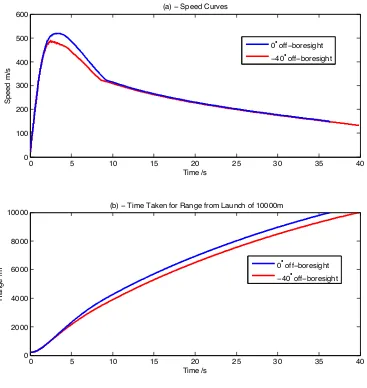
4.4 Speed Curve comparison of off-boresight angles of 0◦ and −40◦ . . 71

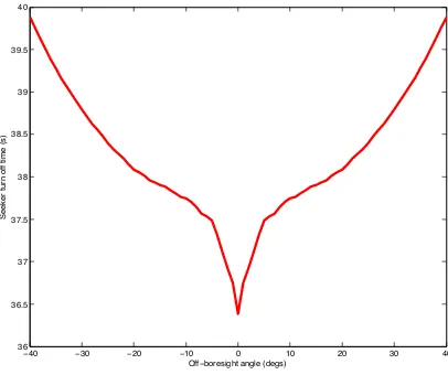
4.5 Seeker turn off time as a function of the launch off-boresight angle 72 4.6 Predicted target locations at 35s . . . 73

4.7 Total probability of intercept considering only the scan area asso-ciated with a direct attack . . . 74

4.8 Kalman Filter Example . . . 89

4.9 Typical Target Trajectory . . . 103

4.10 Ground Truth Data for a Typical IMM Run . . . 103

4.11 Associated Mode Probabilities . . . 104

4.12 ROC Curve Based on 100 runs . . . 106

4.13 Flow diagram for the integrated tracking and prediction system . 109 4.14 Example of Elimination of Predicted Trajectories by the Integrated Tracking and Prediction System . . . 110

5.1 Detectable predicted target locations determined using the 3 di-mensional method . . . 114

5.2 Detectable predicted target locations determined using the 2 di-mensional method . . . 115

5.3 Intercept Probability Distribution for a Single Off-boresight Angle Applied at Times T=0s....T=25s . . . 124

5.4 Intercept Probability Distribution for Two Off-boresight Angles Applied at T=0s and T=10s . . . 125

5.5 Effect of starting temperature on Simulated Annealing Performance129 5.6 Effect of Number of Runs at each Temperature on Simulated An-nealing Performance . . . 130

5.7 Effect of Cooling Constant on Simulated Annealing Performance . 131 5.8 Simulated Annealing - Example Path Taken in a 3 Dimension Op-timisation Process . . . 132

5.9 Feasible Trajectory Solution Area . . . 138

5.10 Feasible Trajectory Solution Area . . . 139

5.11 Typical Simulated Annealing Results at Weapon Initialisation . . 141

5.12 Data Link Activity for 0 Manoeuvre Detections by the IMM . . . 143

5.13 Data Link Activity for 1 Manoeuvre Detection by the IMM . . . . 144

5.14 Data Link Activity for 4 Manoeuvre Detections by the IMM . . . 146

(11)

5.17 S.A.S.S - Example Engagement Plot Set 1 . . . 150

5.18 S.A.S.S Example Engagement Plot Set 2 . . . 151

5.19 S.A.S.S results . . . 153

5.20 IMM Detections for each Simulated Engagement . . . 157

5.21 IMM Miss Detections . . . 158

5.22 S.A.S.S Failure Due to Scan Area Orientation . . . 160

6.1 Example Calculation of an Updated Target Trajectory in the M.P.T System and Associated Off-boresight Command . . . 164

6.2 Example Engagement of a Manoeuvring Target using the M.P.T Integrated Fire Control System . . . 165

6.3 Example Engagement of a Manoeuvring Target using the M.P.T Integrated Fire Control System plot set 2 . . . 166

6.4 M.P.T results . . . 168

6.5 Weapon Overcommitment in M.P.T Integrated Fire Control Sys-tem . . . 170

6.6 M.P.T System Component Fails . . . 172

(12)

List of Tables

3.1 Fire and Forget (F.F) System Results . . . 55

4.1 True State Data for a Typical Random Target Trajectory . . . 104

4.2 IMM Mode Detection Data for a Typical Random Target Trajectory105 4.3 IMM Confusion Matrix for 100 Random Target Trajectories . . . 105

5.1 S.A.S.S and F.F Results . . . 154

5.2 Observed Data . . . 155

5.3 Expected Data . . . 155

6.1 M.P.T and F.F Results . . . 168

(13)

List of Abbreviations

A.T.T Able to Transmit

Bo Boost Guidance Phase

C.T.L Coordinated Turn Left

C.T.R Coordinated Turn Right

C.V Constant Velocity

D Target Detectable

I.B.M Intercept Before Manoeuvre

I.F.T.R Inflight Trajectory Revision

Mi Midcourse Guidance Phase

M.T Manoeuvring Target

N.D Not Detectable

N.A.T Not Able to Transmit

N.M Non Manoeuvring Target

M.P.T Most Probable Trajectory

P.S.A Predicted Scan Area

W.I Weapon Initialisation

(14)

S.A Simulated Annealing

S.A.S.S Simulated Annealing and Simple Search

S.A.M.P.T Simulated Annealing and Most Probable Trajectory

(15)

Acknowledgements

I would like to thank my supervisor Dr Jason Ralph for his support, advice and encouragement for the duration of my PhD as well as the introduction to some excellent single malts.

Special thanks go to Dr Neil Oxtoby whose support and words of wisdom through the first two years of the PhD helped me to progress through some of the most difficult aspects of the research.

I am also grateful to Dr Ralph and the Department of Electrical Engineering for their financial support.

(16)

Chapter 1 Introduction

World War II saw the first operational use of a guided weapon, when the German Luftwaffe successfully deployed the Fritz X radio controlled bomb against the Italian Battleship Roma on the 21st July 1943. The Fritz X was equipped with moveable control surfaces, which could be deflected by an operator sending con-trol signals over a radio link. By deflecting the concon-trol surfaces the bomb could be steered onto the target thereby increasing the probability of a successful strike [1].

In the 70 years since the deployment of the Fritz X, guided weapon technology has advanced rapidly with an assortment of weapons being developed to fulfil a variety of roles and operational requirements across a wide range of launch plat-forms. The configuration of a guided weapon depends on a number of factors such as the desired weapon stand off range, operating conditions and launch platform.

For example, the Storm Shadow missile was developed as a long range, air launched cruise missile, which is deployed against high value targets. The long stand off range (maximum range at which the weapon can be launched such that it can reach its intended target [2]) allows the aircraft to engage a target beyond the engagement range of enemy air defence systems thereby increasing the surviv-ability of the launch platform itself [3]. Another example of a guided weapon is the Sea Wolf missile system which is designed as a last resort naval point defence weapon to destroy enemy ships, aircraft and missiles [4].

(17)

has changed or disappeared.

The Brimstone Missile system for example, was originally selected to meet the RAF requirement for a long range Anti-Armour Weapon in 1997. This require-ment was identified from the substantial use of tanks and armoured vehicles by Iraq forces during the 1st Gulf War. However the weapon only entered into ser-vice in 2005 after a development cost of£370 million [5], by which time the Gulf War was over.

Over the past few years a requirement to be able to intercept highly manoeu-vrable relocatable targets has emerged [6], especially within Naval operations as demonstrated by the emergence of the small boat threat [7]. As the defence budgets of prominent military powers such as the UK and the USA continue to shrink, greater emphasis is being placed on adapting current legacy systems to respond to new operational requirements such as these.

In 2006, an Enhanced Paveway II (ePwyII) bomb was fitted with a data link and released from a Tornado GR4 aircraft [8]. In a standard ePwyII bomb the weapon would have followed a trajectory to a preset target location. The tra-jectory flown by the weapon would have been governed by the onboard guidance system.

However in this weapon trial the target co-ordinates where updated in flight using the data link. The bomb would then have performed one or more manoeu-vres thereby changing the shape of its trajectory in order to reach the updated target location. The trial was successful, with the weapon successfully flying to the updated target location.

The demonstrated ability to shape the trajectory of an inflight data linked weapon has the potential to significantly increase the performance of some legacy systems to intercept highly manoeuvrable targets. One possible candidate for this type of approach is the Advanced Anti-Armour Weapon (AAAW).

(18)

the duration of the weapon fly out (maximum flight time of the weapon).

It is postulated in this thesis that this can be achieved through the use of an integrated fire control system. The system will seek to calculate an optimal shaped weapon trajectory which should maximise the ability of the weapon to respond to target manoeuvres thereby improving the probability of a successful interception occurring.

The potential effectiveness of an integrated fire control system is explored by considering the scenario of a generic data linked AAAW which is to intercept a small agile highly manoeuvrable surface vessel.

1.1 Structure of thesis

This thesis is divided into seven chapters :

• Chapter 2 - Weapon Model, describes the fundamental concepts associated with tactical missile design and the specification of the AAAW model.

• Chapter 3 - The Small Boat Threat, discusses a realistic target model rep-resentative of a small boat threat. A performance evaluation of the AAAW as a Fire and Forget system using 80 random target trajectories is provided.

• Chapter 4 - Integrated Tracking and Trajectory Prediction, describes the design and implementation of an integrated tracking and target trajectory prediction system

• Chapter 5 - Integrated System One (S.A.S.S), describes the design, im-plementation and results of the first integrated fire control system to be discussed in the thesis.

• Chapter 6 - Integrated System Two (M.P.T), describes the design, imple-mentation and results of the second integrated fire control system to be discussed in the thesis.

• Chapter 7 - Integrated System Three (S.A.M.P.T), describes the design, implementation and results of the final integrated fire control system to be discussed in the thesis.

(19)

1.2 Original contributions of this thesis

The contribution of this thesis is to demonstrate that an integrated fire control system can significantly improve the performance of a weapon against manoeu-vring targets.

Though the focus of the research is the scenario of an AAAW intercepting a small boat, the techniques and systems discussed in the thesis can potentially be applied to a wide range of targets and weapon systems.

(20)

Chapter 2 Weapon Model

The research discussed in this thesis is based around a fixed launcher Advanced Anti Armour Weapon (AAAW) which is simulated using the Matlab program-ming language. The AAAW model is classed as a tactical missile. The details surrounding the model itself and the justification for its selection in this particular project will become apparent later on in the chapter. However many of the con-cepts and much of the terminology surrounding tactical missiles will be unknown to the non expert. Therefore the purpose of this chapter is firstly to present a brief overview of these fundamental concepts such as aerodynamics, weapon guidance and control and rocket propulsion and then to outline the specifics of the model and its role within this research project, beginning with the definition of a missile.

2.1 The Main Components of a Tactical Missile

A missile can be defined as a self propelled aerospace vehicle designed for the purpose of inflicting damage on a designated target [11]. There are two main classes, strategic and tactical. Strategic missiles are long range weapons designed to inflict a significant amount of damage onto a target, with the most widely recognised form of strategic missile being the intercontinental ballistic missile (ICBM), which carries a high yield nuclear warhead. Tactical missiles are gener-ally much smaller weapons, carrying conventional warheads and are used against specific threats such as aircraft, ships and enemy missiles.

(21)

cruise missile.

The AAAW model is of the tactical class, which having a fixed launcher sys-tem will always be launched at the same pitch, yaw (heading) and roll for each engagement. By considering a fixed launcher, the performance of the integrated fire control systems discussed in later chapters is then dependent only on the mis-sile sizing and associated aerodynamic capability and the quality of the weapon trajectory optimisation methods.

2.2 Basic Aerodynamics and Fundamental

Con-cepts

A dynamic model describes the motion of the missile within one or more degrees of freedom. Each degree of freedom describes either the translational or rotational motion of the airframe. The number of degrees of freedom used depends on the specific application of the model. The greater the number of degrees of freedom which are used to describe the motion, the more computationally intensive the model will be. This will be due to the increased number of equations required to be solved to model the airframe dynamics. The choice of model is therefore determined based on the user’s requirements.

The dynamics of a missile airframe are normally modelled assuming rigid body dynamics [13] which for general spatial motion results in three translational and three rotational degrees of freedom. This is known as a Six Degrees of Freedom (6DoF) model.

In a 6DoF model the translational motion is described as translation in (X, Y, Z) with the rotational motion defined in terms of three angles (pitch θ, heading ψ

and roll φ). However if only the longitudinal motion of the weapon was of inter-est e.g. in an assumed planar engagement, then the dynamics could be modelled using a 3DoF model [14], considering only the translation of the airframe in the

X and Z axis and the weapon pitch.

Different combinations of translational and rotational motion can be used to define a variety of dynamic models. An overview of the most common dynamic models used in missile simulation today can be found in [15].

(22)

both longitudinal and lateral guidance commands to be generated. The weapon is a roll, stabilised missile, requiring roll stabilisation commands to be generated by the guidance computer. Therefore a full 6DoF model is required to model the motion of the missile airframe using three translational and three rotational degrees of freedom.

A 6DoF model requires the rate of change of both the translational and rota-tional degrees of freedom to be determined. The associated variables for the translational and rotational movement are the translational velocities and accel-erations and the Euler angle rates.

The translational velocities (vx, vy, vz) and accelerations (ax, ay, az) are relatively

simple to determine, they are the first and second time derivatives of the airframe position in 3DoF. The Euler angle rates ( ˙ψ,θ,˙ φ˙) (defined in Earth-orientated axes) however are more complicated to determine. The Euler rates are func-tions of the angular velocities (P, Q, R) (defined in body orientated axes) and the weapon attitudes. The Euler rates are calculated using the following equa-tions [16] :

˙

φ=P +Qsinφtanθ+Rcosϕtanθ. (2.1) ˙

θ =Qcosφ−Rsinφ. (2.2) ˙

ψ =Qsinψ

cosθ +R

cosψ

cosθ (2.3)

The dynamics of the missile are dependent on the aerodynamic forces and mo-ments which act on the airframe during flight. The aerodynamic forces as well as the moments are produced by the variations in pressure and velocity due to the flow of air around the missile. The propulsive force (i.e thrust) is generated from the propulsion system on the missile.

(23)

The Drag force is produced by the pressure and skin forces which act on the surface of the missile. It acts parallel to the free stream velocity [11].

The Lift force is produced by the pressure forces acting on the surface of the missile. It acts perpendicular to the velocity vector of the missile and to the free stream [11].

The Side Force is the component of the resultant aerodynamic force which acts perpendicular to the lift and drag forces [11].

Three moments consisting of the Pitching, Yawing and Rolling moments are also defined which are created by varying the aerodynamic load distribution on the airframe using a control scheme.

2.3 Axes Systems

There are three important axes systems which are used within missile flight sim-ulation consisting of the Earth, Body and Wind axis systems.

The Earth axes is a right handed system [11] which is used to determine the true position of the missile at every time step during the simulation. TheX and

Y axes lie in the horizontal plane (Xe, Ye), with the Z axis pointing vertically

down in the direction of gravity (Ze). The Earth axes system [17] is shown in

(24)

APPENDIX C - Continued

X_t Lie in geometric plane of y_) Earth's surface

p- Nonrotati.ng E }

Figure 164.- Earth-axis system.

Body-Axis System

In the body-axis system the rectangular Cartesian axis system is oriented such

that the X-axis points out of the nose of the aircraft and is coincident with the longi-tudinal axis of the aircraft. The Y-axis is directed out of the right wing of the

air-craft and the Z-axis is perpendicular to both the X and Y axes and is directed downward. The origin of the entire system is taken to be the center of gravity of the

aircraft. At this point it is useful to define the important angular displacement terms

roll, pitch, and yaw.

Roll: the airplane rotates about its longitudinal axis (that is, X-axis). A positive roll is defined as the Y-axis turning toward the Z-axis, that is,

the right wing drops.

Pitch: the airplane rotates about the Y-axis. A positive pitch is defined as

the Z-axis turning toward the X-axis, that is, the nose of the airplane rises.

Yaw: the airplane rotates about the Z-axis. A positive yaw is defined as the

X-axis turning towards the Y-axis, that is, the nose moves to the right (clockwise when viewed from above).

194

Figure 2.1: Earth Axes

The missileBodyaxes is a right handed system which is used for calculating the aerodynamic forces and moments, with an origin defined by the missile centre of gravity. The X axis coincides with the longitudinal axis of the missile (Xb).

The positive Y axis is positive to the right and lies perpendicular to the X axis (Yb). TheZaxis is positive downwards (Zb) and is perpendicular to theXY plane.

Three rotations are also defined within this axes system, which are known as the Rollφ, Pitch θ and Yawψ.

1. Roll is a rotation about the Xb axis.

2. Pitch is a rotation about the Yb axis.

3. Yaw is a rotation about the Zb axis.

(25)

APPENDIX C - Continued

The body-axis system and the concepts of roll, pitch, and yaw are illustrated in figure 165.

YB

XB Roll

Yaw

Z B

Figure 165.- Body-axis system.

Wind-Axis System

In the general wind-axis system, the origin of the rectangular Cartesian system is at the center of gravity of the aircraft. The X-axis points into the direction of the oncoming free-stream velocity vector. The Z-axis lies in the plane of symmetry of the airplane and is perpendicular to the X-axis and is directed generally downward. The Y-axis is perpendicular to both the X and Z axes (fig. 166(a)). In many prob-lems of interest airplane motion is in the geometric plane of symmetry (no yawing motion) so that the X-axis also lies in the plane of symmetry. This means that the Y-axis points out of the right wing. The Z-axis again is in the plane of symmetry. The system then is termed the simplified wind-axis system and is illustrated in fig-ure 166(b)).

195

Figure 2.2: Body Axes

The Windaxes is right handed system which is used for the calculation of aero-dynamic coefficients. The X axis in the system is positive in the direction of the free stream Xw. The Y axis is perpendicular to the X axis and positive to the

right of theX axisYw and theZ axis is positive downwards perpendicular to the XY plane Zw. The missile/aircraft centre of gravity lies at the origin of the axes

(26)

APPENDIX

C - Concluded

Yw

Relative wind not in )'7 jc/Xw

Zw

the plane of symrnetry//_

(i"

(a)

General

wind-axis

system.

Z-axis

in plane

of

symmetry.

Yw

f

(b)

Simplified

wind-axis

system.

X

and

Z

axes

in plane

of

symmetry.

[image:26.612.162.493.69.321.2]

Figure

166.-

Wind-axis

system.

Figure 2.3: Wind Axes

During the missile simulation, variables such as the position and velocity in the Earth axes will be transformed into the Body axes position and velocity and vice versa. This is accomplished by multiplying the defined missile position vector in the Earth axes by rotation matrices in heading, pitch and roll about the bodyX

axis,Y axis andZ axis respectively. Rotations in heading (ψ), pitch (θ) and roll (φ) are calculated as follows [13] :

  X0 Y0 Z0  =  

cosψ sinψ 0

−sinψ cosψ 0

0 0 1

    X Y Z   (2.4)   X0 Y0 Z0  =  

cosθ 0 −sinθ

0 1 0

sinθ 0 cosθ     X Y Z   (2.5)   X0 Y0 Z0  =  

1 0 0

0 cosφ sinφ

0 −sinφ cosφ     X Y Z   (2.6)

The Earth coordinate system to Body coordinate system transformation matrix

Tb

e is then expressed as the multiplication of the following matrices [15]:

T_eB=

 

1 0 0

0 cosφ sinφ

0 −sinφ cosφ  

 

cosθ 0 sinθ

0 1 0

sinθ 0 cosθ  

 

cosψ sinψ 0

−sinψ cosψ 0

0 0 1

 

(2.7) The axes systems used in the weapon model assumes that the earth is flat and static. While both of these assumptions are approximate, they only become a

(27)

problem if distances are long, i.e if the trajectory of an ICBM was to be deter-mined the curvature of the earth and its rotation would have to be considered. The Advanced Anti Armour Weapon model used in this thesis has a range of less than 11000m therefore these approximations are acceptable.

2.4 Aerodynamic Force and Moment Equations

The forces and moments which act on the missile airframe, are calculated using the equations of motion for a rigid body. The use of a rigid airframe model is an approximation. An actual missile would flex slightly during flight. However the error induced in the calculated values for the forces and moments will only be very small as missiles are designed to withstand high lateral G-forces [13]. The use of a rigid body simplifies the calculation of the forces and moments consider-ably.

TheDrag(Fx),Side(Fy) andLift(Fz) forces are defined mathematically as [18]

:

Fx =−qS(CDcosαcosβ+CY cosαsinβ−CLsinα)−mgsinθ+T. (2.8)

Fy =−qS(CDsinβ−CY cosβ) +mgcosθsinϕ. (2.9) Fz =−qS(CDsinαcosβ+CY sinβ+CLcosα) +mgcosϕ. (2.10)

where :

q = Dynamic Pressure (P a)

S = Reference Area (m2₎

T = Thrust (N)

m = Mass of the weapon (kg)

g = Gravity constant of 9.81 (m/s2₎

α = Angle of attack (rads)

β = Angle of side slip (rads)

CD = Aerodynamic drag coefficient defined in the wind axis (dimensionless)

CY = Aerodynamic side force coefficient defined in the wind axis (dimensionless)

(28)

ThePitching (M),Yawing (N) and Rolling (L) moments are defined as [18] :

M =qSbCm. (2.11)

N =qSbCn. (2.12)

L=qSbCl. (2.13)

where :

b = Reference length (m)

Cm = Aerodynamic pitching moment coefficent (dimensionless)

CY = Aerodynamic yawing moment coefficient (dimensionless)

CL = Aerodynamic rolling coefficient (dimensionless)

The mathematical representation of the forces and moments has introduced a number of important quantities which must be properly defined and calculated such as, the definition of the reference area and length, the calculation of the dy-namic pressure and angles of attack and side slip. The remainder of this section will provide a brief description of each of the quantities defined in the force and moment equations beginning with the reference area and reference length.

The reference area (S) for a missile is defined as the body cross-sectional area and thereference length (b) is defined as the mean missile diameter [19]. Con-ventionally for an aircraft model, the reference area is defined as a wing plan form area and the reference length is defined as the wingspan for the calculation of the lifting and yawing moments and the mean aerodynamic chord for the calculation of the pitching moment.

The dynamic pressure (q) is calculated from the total airspeed (Va) and the

atmospheric air density (ρ) in kg/m3 _{at a height (}_h _{in metres) as follows [16] :}

q= 1 2ρV

2

a (2.14)

The atmospheric air density is defined as [16] :

ρ= 1.225(1−2.18×10−5h)4.2586. (2.15)

The total airspeed is calculated as :

Va =

q

(29)

where (u, v, w) are the components of the missile velocity vector and (ug, vg, wg)

are the components of the local wind velocity vector.

In order for aerodynamic lift to be generated by the missile, it must achieve an angle of attack [15]. The angle of attack α is defined as :

α = arctan

w−wg u−ug

(2.17)

The angle of sideslip β can be thought off as the directional angle of attack and is calculated from the body X axis and the wind corrected velocity vector as follows :

β = arcsin

v−vg

Va

(2.18)

The angles of attack and sideslip appear in the force equations because the aero-dynamic coefficients for Drag, Lift and Side force are often determined in the wind axes, however the force equations are solved within the body axes. The angles of attack and sideslip are used to correctly express the force coefficients in terms of the body axes instead of the wind axes

The Aerodynamic coefficients are used to calculate the aerodynamic forces and moments which act on the missile in flight [15]. They can be calculated from wind tunnel measurements or using analytical methods. The most common an-alytical method is to calculate stability derivatives which predict how the forces and moments which act on the airframe change as stability parameters such as the angle of attack are varied.

2.4.1 Calculation of Aerodynamic Coefficients

Each aerodynamic coefficient is defined by a set of stability derivatives which can be defined using a first order Taylor series expansion about a trim flight condition. A trim flight condition is a flight condition whereby the forces and moments on the missile sum to zero. The stability derivatives are then determined by considering all of the possible relationships which may exist between the force and moment coefficients and the parameters which affect the stability of the airframe, such as the angles of attack and sideslip. Before defining the aerodynamic coefficients, the calculation of a first order Taylor expansion [20] for a multivariate function is reviewed below :

(30)

2. The Taylor series expansion of the first order would then be defined as :

f(x, y) =f(a, b) +

(x−a)∂f

∂x + (y−b) ∂f ∂y

(2.19)

3. If a = 0 and b = 0, then the expansion becomes :

f(x, y) = f(0,0) +

(x)∂f

∂x + (y) ∂f ∂y

(2.20)

4. This can be more compactly defined as :

f(x, y) =f0+fxx+fyy (2.21)

The equations for each aerodynamic coefficient can then be defined as :

CD =CD0 +CDαα+CDββ+CDδpδp+CDδqδq+CDδrδr+CDδxδx+... CD_α2α

2

+CD_β2β 2

+CD_δ2 pδp

2 +C_D

δ2_qδq2 +CDδ2_rδr2 +CDδ_x2δx2 +... S

2Va

[CDα˙α˙ +CD_β˙β˙+CDpP +CDqQ+CDrR] (2.22)

CY =CY0 +CYαα+CYββ+CYδpδp+CYδqδq+CYδrδr+CYδxδx+... CY_α2α

2₊_C Y_β2β

2₊_C Y_δ2

pδp 2 +C_Y

δ2qδq 2 +C_Y

δ2rδr 2 +C_Y

δ2xδx 2 +... S

2Va

[CYα˙α˙ +CYβ˙

˙

β+CYpP +CYqQ+CYrR] (2.23)

CL =CL0 +CLαα+CLββ+CLδpδp+CLδqδq+CLδrδr+CLδxδx+... CL_α2α

2

+CL_β2β 2

+CL_δ2 pδp

2 +C_L

δ_q2δq2 +CLδ2_rδr2 +CLδ2_xδx2 +... S

2Va

[CLα˙α˙ +CLβ˙

˙

β+CLpP +CLqQ+CLrR] (2.24)

Cm =Cm0 +Cmαα+Cmββ+Cmδpδp+Cmδqδq+Cmδrδr+Cmδxδx+... Cm_α2α

2₊_C m_β2β

2₊_C m_δ2

pδp

2 +C_m δ2qδq

2 +C_m δr2δr

2 +C_m δ2xδx

2 +... S

2Va

[Cmα˙α˙ +Cmβ˙

˙

β+CmpP +CmqQ+CmrR] (2.25)

Cn =Cn0 +Cnαα+Cnββ+Cnδpδp+Cnδqδq+Cnδrδr+Cnδxδx+... Cn_α2α

2

+Cn_β2β 2

+Cn_δ2 pδp

2 +C_n

δ2_qδq2+Cnδ_r2δr2 +Cmδ2_xδx2 +... S

(31)

Cl =Cl0 +Clαα+Clββ+Clδpδp+Clδqδq+Clδrδr+Clδxδx+... Cl_α2α

2₊_C l_β2β

2₊_C l_δ2

p

δ_p2 +C_l

δ_q2δq2 +Clδ_r2δr2 +Clδ_x2δx2 +... S

2Va

[Clα˙α˙ +Cl_β˙β˙+ClpP +ClqQ+ClrR] (2.27)

The rotational derivatives such asCDα˙ are multiplied by S

2Va

as these derivatives are taken with respect to this quantity where S is the reference area and Va is

the total airspeed of the missile [21]. The value of each stability derivative listed in equations 2.22-2.27 is provided in Table 1 of Appendix A. Stability derivatives with a value of 0 indicate that there is no significant relationship between the sta-bility parameter and the respective coefficient. Stasta-bility derivatives with a non zero value are listed as the actual coefficient. This means that either a constant is known for that stability derivative or an expression is provided in [19] which can reliably predict the value of the derivative under various trim conditions.

The actual values of the non zero stability derivatives are sensitive and have therefore been omitted from the thesis.

It should be noted that there are a number textbooks for which expressions for non zero stability derivatives can be obtained (see references [11] and [15]), however [19] should be consulted in the first instance. This is because the text provides a number of reliable expressions for the calculation of several stability derivatives for the moment (Cl, Cm, Cn) and side force (CY) coefficient

expres-sions as well as an in-depth calculation of the drag coefficient. The reliability of these expressions has been verified by comparing predicated values from this text to known parameters for a classified weapon model.

(32)

2.4.1.1 Conventional Weapon Control

Conventional aerodynamic control of a tactical missile is often very different to that of an aircraft. Changes in the roll, pitch and yaw of an aircraft is achieved by using elevators, ailerons and rudders. However the attitudes of a tactical missile (which uses conventional aerodynamic control) are normally manipulated using external control surfaces of which there are three main types, consisting of ca-nards, wings and fins.

Canards are small surfaces located at the front of the body, wings are larger surfaces located within the middle of the body andfinsare small surfaces located at the rear of the body. Other control methods exist, such as, thrust vectoring and reaction jet control which manipulate the direction of the thrust produced by the rocket engine to achieve attitude changes. The choice of control scheme is dependent on a number of factors which are beyond the scope of this thesis, however an in-depth discussion of each control scheme is provided in [19] for the interested reader.

The simulated AAAW in this thesis utilises a conventional fin control scheme. A fin control scheme allows the guidance computer on the weapon to produce four control deflections, which consist of, a required change in pitch (δq), heading

(δr), roll (δp) and drag (δx). Drag control is used in some Laser Guided Bombs

to increase the amount of drag on the bomb to reduce the speed of descent. Drag control is not utilised in the guidance and control scheme of the AAAW model.

(33)

Figure 2.4: + configuration

In the simple case of (+) roll orientated weapon using four control surfaces (as in this model) [19], a pitching moment is created by deflecting fins 2 and 4 which results in a normal force in the direction of the required pitch. A yawing moment is created by deflecting fins 1 and 3 in alternative directions, inducing a side force into the desired yaw direction. A rolling moment is created by deflecting all 4 fins in either a clockwise or counter clockwise direction.

2.4.2 Coefficient of Drag Calculation

The coefficient of drag is the summation of the drag due to the body (CD0body)

control surfaces (CD0controlsurf aces) and stabilising surfaces (CD0stable). Control and

stabilising surfaces consist of wings, fins and canards. A missile can have either 1-3 sets of surfaces, for instance the Starburst missile system [19] has only canards and a tail. This section will explore the calculation of the drag due to the body and then due to the external control and stabilising surfaces.

2.4.2.1 Body Drag

The body drag consists of three parts, the drag due to the shock wave on the nose, the drag due to the body base and the drag due to the body skin friction.

The drag due to the shockwave on the nose is determined based on its geometry, namely the nose length (ln), nose diameter (dn), missile reference area (Sref) and

(34)

number (M) which is calculated as [15] :

M = Va

a (2.28)

whereVais the missile airspeed anda is the speed of sound (which is 343.2 m/s at

sea level and standard atmospheric pressure [15]). The drag due to the shockwave on the nose CD0nose can then be defined as [19] :

CD0nose =

3.6

(ln

d)(M −1) + 3

(Sref −SHemi) Sref

+ 3.6

0.5

M −1+ 3

SHemi

Sref

(2.29)

It is worth mentioning that the drag due to the shockwave on the nose only be-comes significant if the missile is travelling at supersonic speeds, it is relatively small for subsonic speeds.

The drag due to the body base depends on whether the missile is coasting or is powered and if the missile is at subsonic or supersonic speeds when the aero-dynamic drag due to the body base is computed.

If the missile is travelling at supersonic speeds and is coasting then the drag due to the body base (CDBase,Coast) will be [19] :

(CDBase,Coast) = 0.25/M (2.30)

If the missile is travelling at subsonic speeds and coasting then (CDBase,Coast)

becomes [19] :

(CDBase,Coast) = 0.12 + 0.13M 2

(2.31)

However if the missile is powered then the base drag is reduced by a factor of (1−Ae/SRef) (where Ae is the effective nozzle area ). The drag due to the body

base (CDBase,P owered) then becomes [19]:

(CDBase,P owered) = (1−Ae/SRef)(0.25/M) (2.32)

If the missile is travelling at subsonic speeds and is powered then the base drag becomes [19] :

(CDBase,P owered) = (1−Ae/SRef)(0.12 + 0.13M

2₎ _(2.33)

(35)

why the base drag is reduced at both subsonic and supersonic speeds during pow-ered flight.

At subsonic speeds the pressure waves created by the missile passing through the air will be smooth and gradual. The air begins to move out of the way of the missile before the missile reaches it. Therefore at subsonic speeds, the more significant contribution to the body drag in respect of the skin friction and nose shockwave will be the skin friction.

The drag due to the skin friction is a function of the body length (l), dynamic pressure (q) and Mach number (M) and is defined as [19] :

CD0Body,F riction = 0.053(l/d)[M/(ql)] 0.2

(2.34)

As the missile accelerates to the speed of sound, shockwaves appear on the upper and lower surfaces. Once the missile reaches the speed of sound (Mach 1), the shockwaves will arrive at the trailing edge of the airframe. A bow shockwave will also form at the nose. As the missile then accelerates past the speed of sound, the shockwaves on the nose and trailing edge will become more oblique. The drag due to the shockwave on the nose will then become the most significant contribution to the missile body drag at higher than Mach 1 speeds.

2.4.2.2 Drag Due to Control Surfaces and Stabilising Surfaces

There are two components to the drag produced by the aerodynamic surfaces, these are the drag due to the shockwave and the drag due to the skin friction.

The drag due to the shockwave for an external aerodynamic surface is a function of the Mach Number (M), the specific heat ratio (γ), the leading edge sweep and thickness angles (δLE,∆LE), the thickness of the mean aerodynamic chord

(tmac), the span (b) and the number of the specific aerodynamic surfaces being

considered (nw).

Taking the wing as example, the drag due to the shockwave on the wing (if

Mcos ∆LE >1) is defined as [19]:

CD0_wing,wave =nw

2

[(γ(Mcos ∆LE)2)]

((

[(γ+ 1)(M cos(∆LE)2]

2

) γ γ+ 1

(

(γ+ 1)

[2γ(Mcos ∆LE)2 ₋₍_γ₋_1)]

)

1

γ−1

−1

) sin2_γ

LEcos∆LEtmacb Sref

(36)

IfM∆LE <1 then the drag due to the shockwave CD0_{W ing,W ave} is 0.

The drag due to the wing friction CD0_{W ing,F riction} is a function of the number

of aerodynamic dynamic surfaces being considered (nw), the length of the mean

aerodynamic chord (Cmac), the dynamic pressure (q) and the wing platform and

reference areas (SW, SRef). It is defined as follows [19] :

CD0_{W ing,F riction} =nw[0.0133/(qCmac) 0.2

](2SW/SRef) (2.36)

Therefore the total drag due to the wings is equal to:

CD0_{W ing}=CD0_{W ing,W ave} +CD0_{W ing,F riction}

The weapon model in this thesis is fin controlled and uses fixed canards for airframe stabilisation. Therefore the total drag CD0 due to the body and the

aerodynamic surfaces is defined as [19] :

CD0 =CD0_body +CD0_canard +CD0_{f ins} (2.37)

The calculation of the aerodynamic drag coefficient concludes the discussion of the concepts and equations associated with the 6DoF dynamic model. The following sections will discuss the propulsion, warhead, guidance and control considerations.

2.5 Warheads

(37)

2.6 Propulsion

There are a variety of propulsion technologies which can be utilised in the design of a tactical missile. The main technologies are Turbofan/TurboJet, Ramjet and Solid Fuel Rockets [15]. Turbofan/Turbojet engines are the oldest form of air breathing jet engine and are most commonly used for subsonic cruise missiles. For missiles which travel at supersonic speeds of between Mach 2.5 and Mach 5, ramjet technology becomes preferable. However ramjets work by using the en-gine’s forward motion to compress incoming air. Therefore they cannot produce thrust at zero airspeed. In order to utilise a ramjet system, the missile must first be boosted to the ramjet take over speed using a rocket engine. The weapon model in this thesis is assumed to use a solid fuel rocket engine, to reflect the fact, that for the purposes of small to medium tactical missiles, solid fuel rocket motors are most often used. This is due to their simplicity, reliability and ability to produce thrust across the entire Mach range [19]. It is also very simple to produce a varying thrust profile.

Solid fuel rocket engines, like all rocket engines, work on the same Newtonian principle that “to every action, their is an equal and opposite reaction”. The propellent in solid rockets consists of fuel and oxidiser. The fuel and oxidiser mix and burn at high pressure within the propellent storage casing, creating a fluid exhaust in the form of a hot gas. The gas is passed through a supersonic propelling nozzle which uses the heat energy of the gas to accelerate the exhaust to a very high speed. The reaction to this produces thrust pushing the engine in the opposite direction.

Some weapons will have a varying thrust profile such as constant thrust or boost sustain thrust. In a solid fuel rocket engine, this is simple to achieve. The gas produced from the combustion chamber is a function of the burn area of the propellent. A large burn area results in more gas and hence greater thrust and vice versa, the change in burn area over time (burn rate), produces the required time varying thrust profile. To change the burn area, a cavity of different shapes such as a wagon wheel or star can be drilled through the centre of the propellent creating various thrust profiles.

(38)

the surface area of the burnt propellent, the greater the thrust produced.

Star and rod-and-tube cross section shapes are designed to produce the same burning surface area over the duration of the burn time, resulting in a constant thrust. A multi-fin shape is designed to produce a boost-sustain profile, which is achieved from the initial burn surface area increasing rapidly over a given burn time. The burn area will then stabilise and remain constant for the remainder of the propellent burn time.

In terms of modelling the rocket engine for the weapon model, the important concept is the specific impulse. The specific impulse Isp of a rocket engine is

a measure of how energetic the propellent or propellent combination is for that particular engine [24]. It is defined as the thrust (T) per unit mass flow ( ˙mg) of propellant (at the Earth’s surface) as follows :

Isp = T

˙

mg (2.38)

It is given in units of seconds, with typical values for solid fuel rockets being of the order 250s [19]. The AAAW model has a boost-coast profile, which is simply implemented as the rearrangement of the above equation :

T =Ispmg˙ (2.39)

The boost phase has a duration of 3s and boosts the missile to speeds of over Mach 2.

2.7 Guidance and Control

A missile guidance system can be divided into three distinct phases, known as the boost, midcourse and terminal phases [11]. In the boost phase, the missile accelerates from its launch platform. During the midcourse phase, the guidance system will make minor modifications to the trajectory of the missile in order to keep the target within the intercept capability of the weapon. In the terminal guidance phase, the weapon will lock on to the target and will perform rapid manoeuvres to intercept the target.

(39)

2.7.1 Command Guidance

Commanded missiles are guided by commands transmitted from the ground via a command link [25]. The missile and target are tracked by a measurement system such as radar [15]. A guidance computer then calculates the required accelerations and associated control commands required to steer the missile onto a collision course with the target. This type of guidance is referred to as command-to-line-of-sight, the midcourse part of the trajectory will normally be optimised to avoid excessive accelerations in the terminal phase of the engagement [26]. It should be noted that commanded missiles do not have their own seekers they can only execute orders, therefore their accuracy depends on the precision of the tracking system.

2.7.2 Beam Rider

A beam rider system consists of a missile with an on-board seeker, and a launch platform which has a radar or laser source [11]. The radar or laser source detects and tracks the target and launches the missile to engage. The seeker onboard the missile determines whether the missile lies within the centre of the beam. If the missile does not lie within the centre of the beam then its on-board guidance computer will apply controls to realign the missile with the target. As all the required information is extracted directly from the radar, there is no requirement for a command link which results in this type of system being relatively simple to implement. However the missile will often be forced to follow a trajectory that will require strong accelerations in the terminal phase, even if the target itself has not performed evasive manoeuvres [26].

2.7.3 Semi-active Homing

(40)

2.7.4 Active and Passive Homing

To overcome the constant illumination issue found in semi-active homing missiles, active seekers have been developed. Active homing missiles have a seeker which is both a transmitter and detector of radiation, with the most common form being radar [11]. An active homing missile will often have a two phase guidance system. In the first part of the engagement i.e the midcourse phase, the missile will be guided to the target using either command or inertial guidance. Once the target is within range of the seeker, the seeker will lock onto the target and proceed to the terminal phase of the trajectory often using a proportional navigation guid-ance law [26].

There are two disadvantages to this type of system. The first is that active homing missiles are considerably more expensive than other types of weapon. The second is that because the missile seeker is a transmitter as well as receiver, the target will often be able to detect that the missile is locked onto it, therefore covert operation will not be possible.

A passive homing missile works much the same way as an active homing mis-sile, however the seeker is only a detector of radiated energy from the target. For example an infrared homing missile is a system which locks onto the heat generated by a target such as in the anti air role, where the missile locks onto the heat produced by the aircraft’s engines.

2.8 AAAW - Guidance System

The weapon model in this thesis is classed as an active homing system, utilising a proportional control scheme and a radar seeker to detect and track targets. The guidance system is activated once the weapon has left the launcher. The missile will first climb to a predefined ride height (boost phase), at which point the midcourse guidance phase will begin. The weapon will now be unpowered and will therefore coast for the remainder of the flight. At a weapon range from launch of 3000m the radar seeker will be turned on. The seeker will now be in target detection mode which means it will scan for a potential target.

(41)

maxi-On the successful detection of a target the seeker will enter the tracking mode and the weapon will begin the terminal guidance phase. The accelerations ap-plied during this guidance stage will cause the weapon to lose altitude. The commanded accelerations will also manoeuvre the weapon to maintain the target within the seeker scan area during this final guidance phase. This is because the seeker is used to determine the position and velocity of the target which are required in order to calculate the appropriate accelerations. The accelerations for the terminal guidance stage are calculated using a Proportional Navigation (PN) law.

2.8.1 PN Guidance Law

Proportional navigation (PN) is the most widely used guidance law in use today [27]. The basic principle of PN guidance is to generate a missile acceleration “which will nullify the line-of-sight (LOS) rate between the target and intercepter [27] ”, where the line of sight R~LOS is defined as vector between the position of

the intercepter (R~i) and the position of the target (R~T).

~

RLOS =R~T −R~i (2.40)

The guidance law [28] can then be expressed as :

~ac= N

R2((R~LOS ×V~C)×V~i)−~g (2.41)

where a~c is the required airframe acceleration,V~C and V~i are the closing velocity

and intercepter velocity respectively, N is the navigation constant and R is the range from the weapon to the target. The gravity bias term ~g insures that the “intercepter is not pulled under the target in the terminal phase of the engage-ment” [28].

2.9 Fire and Forget AAAW Operation

The AAAW model used in this research was originally designed to be representa-tive of a Fire and Forget Anti-Tank weapon for an unrelated project. The weapon can either be launched on or off-boresight. An on-boresight launch is simple, the weapon will maintain the same yaw angle as the launcher once separation has been achieved. Anoff-boresightlaunch consists of the weapon executing a turn right or left after separation which will place the missile on a new heading. The new heading is referred to as the off-boresight angle Ob and is calculated as :

(42)

where ψ is the missile launcher yaw angle and ∆ψ is the required missile yaw change. The missile launcher heading and off-boresight angle are set at the be-ginning of the flight simulation. In this research, the missile launcher heading is always set at 0◦ to represent a fixed launcher situation. This means that the ini-tial yaw of the missile before a potenini-tial off-boresight command is iniini-tialised as 0◦.

If an off-boresight launch is simulated then the off-boresight command is executed by the weapon control system once the simulation clock reaches 1s. This time delay simulates the weapon clearing the launcher. The respective off-boresight angle is then achieved using a yaw control, which requires the deflection of two fins as previously shown in Figure 2.4.

In order to achieve a required fin deflection, gas is expended from a small tank on the missile which in turn moves the fin. The weapon has a limited amount of gas. Therefore the fins can only be deflected a limited number of times during the course of the missile flight. However the fins are responsible for the control of the weapon during all three guidance phases. Because of this, the weapon is restricted to a maximum launch off-boresight angle of 40◦ to ensure that the fins can deflected a sufficient number of times in order to facilitate weapon control during the midcourse and terminal guidance phases. The 40◦ limit was imposed in the original design specification. The AAAW can be launched with an off-boresight angle in the range of±40◦.

As the weapon in this case is simulated as a Fire and Forget system, no further off-boresight commands can be transmitted to the weapon once the simulation has begun. The weapon seeker is aligned to the centre of the missile airframe. The choice of an on-boresight or off-boresight launch will then dictate where the seeker will scan for a potential target.

2.9.1 Scan Area Prediction

In the weapon model the seeker, is simulated as a radar spot on the ground which is scanned back and forth continuously. The seeker scan will scan a limited area (within the xy plane) in front of the weapon as it flies. Only targets which have been successfully detected within the scan area at a given scan time can therefore be engaged and potentially intercepted by the AAAW. The x and y bounds of the seeker scan area are a function of the ride height (Rh), missile heading (ψ),

the seeker depression angle (θd) and the positive and negative seeker sweep angle

(43)

Figure 2.5: Scan Pattern Calculation

The coordinate limits of the scan area can then be calculated using equations 2.43 and 2.44 respectively.

x=x1 =x2 =Rhtan(90−θd) (2.43)

y±= ( q

x2₊_R2

h) tan(±α) (2.44)

In order to account for the heading of the missile, the x and y seeker limits are assembled as a vector and rotated using the following matrix :

cosψ −sinψ

sinψ cosψ

(44)

0 5000 10000

−100

−50 0 50 100

(a) − T = 7s

0 5000 10000

−100

−50 0 50 100

(b) − T = 20s

0 1000 2000 3000 4000 5000 6000 7000 8000 9000 10000 11000

−100

−50 0 50 100

(c) − T = 36.2s

[image:44.612.123.508.85.460.2]

Weapon Trajectory Area Scanned

Figure 2.6: Scan Pattern Calculation

In Figure 2.6 (a), the weapon range from launch is 3000m and therefore the seeker has been activated. In Figure 2.6 (b), the weapon has been in flight for 15s and, as can be seen from the plot, a large area has now been scanned by the seeker. In Figure 2.6 (c), the weapon has been in flight for 36.2s and is now 10000m from the launch point. The seeker has therefore been deactivated. It can be seen, from the Figure that applying an off-boresight angle will therefore change where the seeker will scan for a target for the duration of the weapon fly out.

(45)

weapon INS guidance system such as the Novatel UIMU-LN200 [29]. This system has an operating frequency of 200Hz which is equivalent to an integration period of 0.005s. The calculation of a weapon trajectory and associated scan area takes approximately 3s based on the PC specification outlined in Appendix B.

2.9.2 On or Off-Boresight Launch Selection Criteria

The AAAW model was originally designed to be initialised at the point that a target had been detected from a separate sensor system. The target range, speed and heading of the threat where therefore known. In order to launch the weapon, an appropriate off-boresight angle (if required) is determined by considering a predicted target trajectory and the weapon reachable set.

2.9.2.1 Target Trajectory Prediction

As the weapon model was developed to be representative of in service Anti-Armour Weapons, it was therefore designed to engage the type of targets that this class of weapon would be deployed against operationally. Anti-Armour weapons are used to engage targets which normally travel relatively slowly and in straight lines and/or constrained to terrain features such as roads [30]. Examples of this type of target are vehicles such as Main Battle Tanks, Air Defence Units and Armoured Personnel Carries.

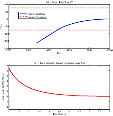
The weapon has a maximum flight time of approximately 40s, so will therefore engage the target in a short space of time.

The predicated target trajectory is calculated by assuming that the target will maintain the detected heading and speed for a duration of 40s, in essence the target will travel in a straight line. As the manoeuvrability of targets such as a Main Battle Tank is poor compared to the weapon, then even if the target does manoeuvre it will not significantly deviate from the predicted trajectory over such a small time period.

Once the predicted trajectory has been determined the appropriate off-boresight angle (if required) can be calculated by using the reachable set.

2.9.2.2 Reachable Set Calculation

(46)

[image:46.612.130.517.169.491.2]

seeker scan area for each off-boresight angle value and joining the respective scan areas together results in the reachable set of the weapon. The reachable set represents the maximum detection boundaries of the seeker and is shown Figure 2.7.

Figure 2.7: Reachable Set with a Missile Launcher Heading of 0◦

In order for the weapon to intercept a target, the target must have one or more points along its trajectory whereby it can be detected by the seeker within the boundaries of the reachable set.

2.9.2.3 Combination of Reachable Set and Predicted Target Trajec-tory

(47)

The off-boresight angle is incremented in steps of 1◦ until one or more valid detection points are determined for a given scan area. A valid detection point is simply when the target at a given time step will lie within the area being scanned by the weapon at the same time step. This requirement is depicted in Figure 2.8.

2000 3000 4000 5000 6000 7000 8000 9000 10000

−6000 −4000 −2000 0 2000 4000 6000 8000

X /m

Y /m

(b) − Target Detection in Reachable Set

9000 9050 9100 9150 9200 9250

1050 1100 1150 1200 1250

X /m

Y /m

(a) − Zoomed in Target Detection

Target Trajectory Reachable Set Target Postion at 31.5s Scan Area at 31.5s Total Scan Area

(48)

In Figure 2.8, the initial target position has been set at the Cartesian [x(0), y(0)] co-ordinate of [9920,1218]. The velocity of the target is 26m/s which is repre-sentative of the maximum road speed of a modern light tank such as the FV 107 in service with the British Army [31], the velocity components [vx(0), vy(0)] are

[−25.85,−2.717]. The predicted trajectory is then calculated using the following expression :     x vx y vy    

(t+dt) =

   

1 dt 0 9 0 1 0 0 0 0 1 dt

0 0 0 1

        x vx y vy    

(t) (2.45)

where t = the prediction time and dt is the prediction time step. The matrix within this expression is a constant velocity model [32]. A target which obeys this model will, maintain the same velocity for the 40s period hence the prediction of a non manoeuvring target trajectory. A time step (dt) of 0.005s is used to define the target at each point along the predicted trajectory. This time step is used to match the integration time for the weapon model. Based on the predicted trajectory, an off-boresight angle of 7◦ has been determined. This will result in a target detection by the seeker at 31.5s provided that the target follows the constant velocity prediction.

(49)

Y

Y Target State

T=0

Weapon State T = 0

Calculate Predicted

Trajectory Determine Off -Boresight angle

Y

N T = T + dt

Target Intercepted ?

Weapon R.F.L <10km ?

End Weapon Simulation Update Weapon

State

Update Target State

N N

Y

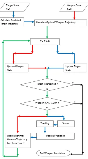
Figure 2.9: Fire and Forget AAAW flow diagram

(50)

2.9.3 Fire and Forget AAAW Demonstration

In order to demonstrate how the AAAW model engages a typical non manoeu-vring target, a simulation was performed with the target following the predicted trajectory determined in section 2.9.2. The results of the simulation are displayed using various plots in Figures 2.10 and 2.11.

In Figure 2.10 (a) the trajectory of the missile during the boost (W.T.B), mid-course (W.T.M) and terminal (W.T.T) guidance phases is shown.

In Figure 2.11 (a) the target detectability during the three guidance phases is shown. A state of N.D means that the target is not detectable by the seeker, in that the target does not lie in the area being scanned by the seeker at that point in time. A state of D means that the target is within the scan area of the weapon and is detectable. The seeker mode during the three guidance phases is depicted in Figure 2.11 (b). The seeker is either off (S/O), in detection mode (S/D) or in tracking mode (S/T).

The weapon altitude, speed, heading and range is shown for the boost (Bo), midcourse (Mi) and Terminal (Te) guidance phases.

(51)

Figure 2.10: AAAW successful direct attack strike, (plot set 1)

(52)

Figure 2.11: AAAW successful direct attack strike (plot set 2)

The seeker is in the detection mode during the midcourse guidance phases. As can be seen from Figure 2.11 (b) the seeker entering the tracking mode and the weapon beginning the terminal guidance phase happens simultaneously. The weapon altitude and yaw plots depicted in subplots (c) and (e) respectively indi-cate an underdamped control law.

Integrated target tracking and weapon guidance