Article
An Efficient Algorithm for Earth Surface
Interpretation from Satellite Imagery
Lawankorn Soimart
aand Mahasak Ketcham
b,*
Faculty of Information Technology, King Mongkut’s University of Technology North Bangkok
,
Bangkok, Thailand
E-mail: a[email protected], b[email protected] (Corresponding author)
Abstract.Many image segmentation algorithms are available but most of them are not fit for interpretation of satellite images. Mean-shift algorithm has been used in many recent researches as a promising image segmentation technique, which has the speed at O(kn2)
where n is the number of data points and k is the number of average iteration steps for each data point. This method computes using a brute-force in the iteration of a pixel to compare with the region it is in. This paper proposes a novel algorithm named First-order Neighborhood Mean-shift (FNM) segmentation, which is enhanced from Mean-shift segmentation. This algorithm provides information about the relationship of a pixel with its neighbors; and makes them fall into the same region which improve the speed to O(kn). In this experiment, FNM was compared to well-known algorithms, i.e., K-mean (KM), Constrained K-mean (CKM), Adaptive K-mean (AKM), Fuzzy C-mean (FCM) and Mean-shift (MS) using the reference map from the Landsat. FNM provided better results in terms of overall error and correctness criteria.
Keywords: Landsat, mean-shift algorithm, segmentation, remote sensing.
1.
Introduction
Remote sensing is the acquisition of information about the earth surface without touching objects in the earth so-called satellite image. Satellite image and aerial image have different recording and objective. An aerial image can directly demonstrate everything in the area from the top such as trees, grasses, roads, and river flows. In contrast, a satellite image is recorded in a long-distance from the land. Regions within the satellite image originate from radiation of the sun. The reflection of energy in one region is used to check the spectral value in order to distinguish one region over other regions. This process is called Passive Remote Sensing [1] as shown in Fig. 1. Most passive sensors use a scanner for imaging, such as Landsat, NOAAH, and MODIS etc. The sensor is equipped with spectrometers for measuring signals at several spectral bands simultaneously, so-called multispectral images which allow numerous interpretations [2]. Recording data for multispectral image depends on weather. The sensor inefficiently records data during raining or high density of cloud. This problem always occurs in tropical countries. Acquisition of multispectral image has low resolution which causes vague interpretation of image. These problems should be solved before interpretation [3].
Fig. 1. Spectral reflectance of satellite.
Interpretation of a satellite image is divided into human approach and computer approach [4]. Human approach needs expert’s profession. The interpreter should have a unique knowledge about the physical zone [5]; and interprets repeatedly which can originate the human-error. Furthermore, the more number of experts increase, the more interpretations are various. In computer approach, interpretation has necessary and sufficient techniques to extract information from the image. The accuracy of computer interpretation is directly affected by the quality of image segmentation [6]. Image segmentation is a great technique in computer vision for partitioning an image into several semantically homogeneous regions [7]. The similar properties of pixels are segmented into the same region. However, dissimilar pixels are grouped in different regions [8-12]. Segmentation algorithms can be applied in many other applications [13] such as image analysis, medical image analysis, pattern reorganization, etc. For satellite images, segmentation can visualize compositions of earth surface which implement for country development in cartography, disaster, oceanography, hydrology, geology, forest, and agriculture etc. [14-15].
Several researches reported application of satellite image segmentation techniques such as K-mean (KM) [7, 16], Constrained K-mean (CKM) [16-17], Adaptive K-mean (AKM) [16], Fuzzy C-mean (FCM) [13, 16, 18-19]. Most of their weakness is either pre-definition for initial number of clusters or outlier.
- Pre-definition of Initial number of clusters: the initial number of clusters is manually predefined by human before segmentation.
- Outlier: in case a group of pixels has less density, segmentation might cluster them as outlier. Or if an area of interest (AoI) is segmented as the outlier, the result of segmentation affects a large number of errors. Outlier filtering is the solution for this process.
1. Sunlight
[image:2.595.182.419.284.455.2]Mean-shift algorithm is a density-based which is simple and flexible for image segmentation. Ordering pixels are ascending then all pixels are grouped into windows. Hence, the pre-definition of clusters is unnecessary. As multispectral satellite image has a number of outliers such as cloudy, rainy and fog. This problem causes many unknown-values of pixels. There are many researches about mean-shift segmentation which not only insufficiently handled the outlier in satellite image but also had high latency time for self-defining the number of clusters [20-24].
In this paper, we propose a novel algorithm named First-order Neighborhood Mean-shift (FNM) segmentation, which is enhanced from Mean-shift segmentation. This algorithm provides information about the relationship of a pixel with its neighbors; and makes them fall into the same region which improve the speed to O(kn).
The contributions of this paper are as follows:
- To eliminate the outlier, we generated the estimation procedure for unknown pixel values using neighbors of pixel.
- To reduce latency time for self-defining the number of clusters, we parallelized similar values of neighbor pixels.
- To improve segmentation with self-defining the number of clusters that can be able to compare in term of correctness with the algorithms with pre-definition.
The rest of this paper is organized as follows: Section 2 provides a preliminary, followed by our proposed algorithm in Section 3. Section 4 has experimental results and discussion. The conclusion and future work are in Section 5.
2.
Preliminary
2.1. Mean-shift Algorithm
A mean-shift algorithm was originally introduced for valley-seeking procedures [22]. Later, this method was used to analyze an image; and essential to segment the composition of image. Moreover this method can use to track moving objects, analysis and clustering.
Mean-shift algorithm can be depicted as Fig. 2. Each color group is a region of the image. The density of each group depends on the mean calculated from density of all pixels in the same group. Each group has a mean value; and each pixel has a pixel value. Each pixel chooses one group that has a mean value similar to its pixel value.
Fig. 2. Mean-shift algorithm [23].
2.2. First order Neighborhood System
Neighborhood system N(s), where sites s∈S refer to each component of the random variable [25-27]. In this work, a first order neighborhood systemN1(s)( 1)
,
where the eight neighborhoods are definedby (1), and visualized by Fig. 3.
1
1 1 1 1 1 1 1 1 1 1 1 1
,
,
,
,
,
,
,
)
(
yx y x y x y x y x y x y x y
x
S
S
S
S
S
S
S
S
s
N
[image:3.595.145.451.492.583.2]Fig. 3. First -order neighborhood system [26].
3.
Proposed FNM Algorithm
This section describes concept of First-order Neighborhood Mean-shift (FNM) algorithm. FNM algorithm is integrated the advantage of first-order neighborhood and mean-shift algorithm. First-order neighborhood can increase the speed of FNM becomes higher than mean-shift algorithm. The system has three main schemes as shown in Fig. 4: Preprocessing, First-order neighborhood and Computational Shifting.
Fig. 4. Diagram of the FNM segmentation.
Converting RGB to Gray Scale
Input a pixel with its 8 neighbors per iteration
Select one pixel from window based on the highest frequency
A B C D
F
N
M
Seg
m
enta
ti
o
n
m
i i x x K n x p
1
2 ) ( 1 ) (
3. Computational Shifting
) ( () ) 1
(r t
x f x
Output
Input Satellite Image 1. Preprocessing
[image:4.595.233.358.78.194.2] [image:4.595.162.434.312.728.2]3.1. Preprocessing
The Landsat image is input. For low-level feature analysis of satellite images [28], each pixel of the raw image is converted from RGB to the gray scale values (0-255). Introductorily, gray scale value is a format of image in term of 256-valued brightness. In this paper, we used YIQ color space [29], as in (2), at the Y-axis to convert RGB to grayscale format as in Eq. (3).
B G R Q I Y 312 . 0 523 . 0 211 . 0 322 . 0 274 . 0 596 . 0 114 . 0 587 . 0 299 . 0 (2)
where R, G, B and Y are in the range between 0 and 1, I is between -0.5957 and 0.5957 and Q is between -0.5226 and -0.5226.
ij ij
ij
ij
R
G
B
Y
0
.
2989
0
.
5870
0
.
1140
(3)where Yij is the gray-scale value of a pixel at the position i and j within the image, Rij is the red-parameter of
a pixel at the position i and j within the image, Gij is the green-parameter of a pixel at the position i and j
within the image and Bij is the blue-parameter of a pixel at the position i and j within the image.
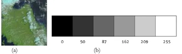
The more the pixel convergence to 0, the more the pixel becomes black. The more the pixel convergence to 255, the more the pixel becomes white, as in Fig. 5.
(a) (b)
Fig. 5. (a) Example of input image and (b) Gray scale range.
3.2. Fist-order Neighborhood
This sub-system has two parameters: group size and number of groups which are inversely dependent as in (4). From Fig. 6, the window has range between 0-255. If the group size is large, the window has a less number of groups. In case of small group size, the window has a huge number of groups. In each iteration, a pixel and its 8 neighbors (according to first-order neighborhood system), are input to the groups of window, where the range of the group is most similar to the pixel value. The highest frequency of group is chosen to store for processing in the next scheme.
[image:5.595.156.475.378.473.2]Fig. 6. Window, group size and number of groups.
3.3. Computational Shifting
As Fig. 4, all pixels of the image are input for computation. In the Mean-shift segmentation, a pixel chooses one group of window to move, where the range of the group is most similar to its pixel value. It computes Eq. (4) and (5), as pixel by pixel overall the image. This method takes long time to segment the region like brute-force at O(kn2). To segment a large-size image, or an image which has a pixel that is similar to many
pixels in the same image. First-order Neighborhood system chooses the representative value from the group instead of overall pixel value. It can solve the speed problem of mean-shift algorithm from O(kn2) to O(kn). The FNM algorithm consists of four main steps as Fig. 7.
Fig. 7. Visualization of computational shifting.
0 255
Group size = 51 Number of groups = 5
Group size = 17 Number of groups = 15 Window = 255
Group size = 255 Number of groups = 5
0 51 102 153 204 255
0 51 102 153 204 255
mean
0 51 102 153 204 255
0 51 102 153 204 255
0 51 102 153 204 255
Step 1.
Step 2.
Step 3.
[image:6.595.147.437.83.201.2] [image:6.595.149.454.357.738.2]Step 1. Compute the density of grayscale value of the group from every pixel which is chosen from the highest frequency of group, using (5). As shown in Fig.8, pixels are substituted by points.
Fig. 8. Window and groups.
(5)
where p(x) is a pixel at position x, n is number of pixels from the image, m is number of groups,
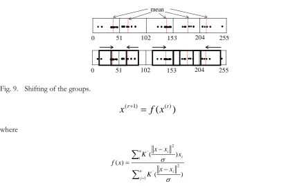
is a window size, K(t) is a kernel density function of the position which has the highest density in the considered area p(x)=0. [image:7.595.133.436.120.239.2] [image:7.595.68.511.319.588.2]Step 2. Calculate the mean of each group to shift the range of the group from (6) and (7), as shown in Fig. 9.
Fig. 9. Shifting of the groups.
)
(
()) 1
(r t
x
f
x
(6)where
n j i i i n i x x K x x x K x f 1 2 ' 2 ' ) ( ) ( ) ( (7)where p(x) is a pixel at position x, n is number of pixels from the image, m is number of groups,
is a window size, K(t) is a kernel density function of the position which has the highest density in the considered area p(x)=0.Step 3.The algorithm stops shifting when the same mean of different groups are partially overlapped, as shown in Fig. 10(a). And the final groups are iteratively reversed to the previous shifting as shown in Fig. 10(b).
0 51 102 153 204 255
m i i x x K n x p 1 2 ) ( 1 ) ( 0 51 102 153 204 255
mean
Fig. 10. Merging of groups and extension of groups (a) Partial overlapping of groups, (b) Reversing of final groups to the previous shifting.
[image:8.595.194.402.287.449.2]Step 4. From the neighborhood system, the pixel chooses one group, and also brings its neighbors which have similar pixel values to move to the same group –so called FNM Segmentation as in Fig. 11.
Fig. 11. Final result of FNM segmentation.
4.
Experimental Results and Comparison
4.1. Experimental Setup
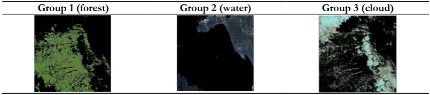
Images used in this experiment were from Landsat dataset with 100x100 pixels and wavelength at 0.45-0.69 µm (visible wavelength). This wavelength could be seen by eyes as blue, green and red. Image segmentation in this wavelength can be obviously segmented cloud, water, and land as shown in Table 1. Each pixel represents 30mx30m physical area.
The image was input to the system. The image was transformed from RGB to Grayscale. The system segmented the image by FNM segmentation. The value of pixel will consider which group the pixel was a member as shown in Fig. 10. In this system, we used 500 images to verify our FNM segmentation in the environment of CPU core i5 and 4GB RAM. The system was implemented by M-script language in Matlab.
Table 1. Detail of output.
Group 1 (forest) Group 2 (water) Group 3 (cloud)
0 51 102 153 204 255
0 51 102 153 204 255
0 51 102 153 204 255
0 51 102 153 204 255
(a)
[image:8.595.76.518.674.772.2]Fig. 12. Grayscale value and groups of output.
4.2. Run-time and Computational Complexity Analysis
4.2.1. Run-time Comparison between FNM and MS
The results and time comparison between Mean-shift and FNM are shown in Table 2 that each image consists of water (grey), forest (black) and cloud (white). The results show that our FNM is more suitable for high variant pixels than Mean-shift because FNM also considers the neighbors for segmentation. In case a pixel value did not recognized any groups, its value could be estimated the membership of one group from its neighbors. In term of time comparison, FNM has less processing time than mean-shift. In FNM, only the redundant value of pixel is selected as a representative into the group. However, Mean-shift has higher computational complexity because the iterations for computation have a large number for all pixels.
Table 2. Result and processing time between mean-shift and FNM segmentation.
Original Image Result Mean-shift Time Result FNM Time
12.83 10.97
15.71 11.12
.
.
.
.
.
.
.
.
.
.
.
.
.
.
.
Average 16.56 Average 11.48
46 171 52 49 50
40 178 179 52 49
114 53 173 170 184
48 56 183 171 171
51 53 53 48 51
1 3 1 1 1
1 3 3 1 1
2 1 3 3 3
1 1 3 3 3
1 1 1 1 1
grayscale value 5x5 pixels groups of output 5x5 pixels
[image:9.595.65.534.450.725.2]4.2.2. Computational complexities of FNM and other algorithms
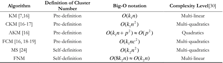
In this section, the computational complexity of FMM was compared with the other well-known segmentation algorithms, i.e., mean (KM) [7, 16], Constrained mean (CKM) [16-17], Adaptive K-mean (AKM) [16], Fuzzy C-K-mean (FCM) [16, 18-19] and Mean-shift (MS) [24]. These algorithms are divided into two groups: Pre-definition of cluster number (KM, CKM, AKM and FCM) and Self-definition of cluster number (MS and FNM). Introductorily, a high computational complexity needs more run-time for algorithm execution [30]. A mathematical asymptotic-notation named Big-O was used for complexity analysis as shown in Table 3. The Big-o parameters are k1, k2, n, p and c.
- k1 is a number of average iteration steps in pre-definition cluster number
- k2 is a number of average iteration steps in self-definition cluster number
- n is a number of data points - p is a number of data dimensions - c is a number of clusters
Table 3. Big-O notation comparison between FNM and other algorithms.
Algorithm Definition of Cluster Number Big-O notation Complexity Level[30]
KM [7,16] Pre-definition O(k1n) Multi-linear
CKM [16-17] Pre-definition
O
(
k
1n
2)
Multi-quadraticsAKM [16] Pre-definition
O
(
k
1n
p
2)
O
(
p
2)
QuadraticsFCM [16, 18-19] Pre-definition
O
(
k
1nc
2)
Multi-quadraticsMS [24] Self-definition
O
(
k
2n
2)
Multi-quadraticsFNM Self-definition O(8k2n)O(k2n) Multi-linear
From Table 3, KM and FNM are in the complexity level of multi-linear. AKM is a quadratics. CKM, FCM and MS are multi-quadratics. From the Big-o notation, multi-linear has the least computational complexity because the multiplied-growth function equals as k1n and k2n. Meanwhile, quadratics (as p2) and
multi-quadratics (as k1n2, k1nc2 and k2n2) need more multiplied-computation than multi-linear. Thus, KM
and FNM have the least time complexity. For the comparison between KM and FNM, we consider k1 and k2. However, FNM is an algorithm with automatic self-definition cluster number that is unnecessary to
manually predefine the number of clusters like KM.
4.3. Quality Comparisons between FNM and Other Algorithms
The evaluation of clustering/segmentation structures is the most difficult cluster analysis [31]. In this paper, evaluation of FNM used the reference map as a target class to compare with other well-known segmentation algorithms, i.e., K-mean (KM) [7,16], Constrained K-mean (CKM) [16-17], Adaptive K-mean (AKM) [16], Fuzzy C-mean (FCM) [16, 18-19] and Mean-shift (MS)[24]. The reference map was from Landsat (visible wavelength) in the zone of Dead Sea, Israel which was downloaded from https://earth.esa.int/web/earth-watching/change-detection/content/-/article/the-dead-sea [16]. The evaluation criteria consisted of Overall Error (OE), Commission Error (CE), Percentage Correct Classification (PCC), Precision (Precision), Recall (Recall), F1 Measure (F1), G Measure (G), and Mathew’s correlation Coefficient (MCC) as shown in Fig. 13. Definitions and formulas are shown in Table 4. These metrics have been calculated from TP, TN, FN and FP.
- TP is the number of changed pixels identified correctly. - TN is the number of pixels correctly identified as unchanged.
[image:10.595.64.534.291.425.2]Fig. 13. Evaluation diagram for algorithms.
Table 4. Evaluation criteria [16].
Evaluation
Criteria Formula Definition
Overall Error (OE)
TP FN
FN OE
OE deals with the probability that a changed pixel is wrongly identified as an unchanged
pixel. Commission Error
(CE) TN FP
FP CE
CE deals with the probability that unchanged pixel is wrongly identified as a changed pixel.
Percentage Correct Classification
(PCC) ( )
) ( FN FP TN TP TN TP PCC
PCC identifies the overall accuracy of the proposed method by means of detecting the changed pixels as changed and unchanged pixels as unchanged.
Precision FP TP TP ecision
Pr Precision is referred to the fraction of changed pixels identified correctly.
Recall FN TP TP call
Re Recall is referred to the fraction of changed pixels identified as unchanged.
F1 Measure call esicion call esicion F Re Pr Re Pr 2 1
F1 is a harmonic mean of precision and recall.
G Measure G PrecisionRecall G is a geometric mean of precision and recall.
Mathew’s correlation
Coefficient (MCC) (TP FP)(TN FN)(TP FN)(TN FP)
FN FP TN TP MCC
MCC is an accuracy of precision and recall.
Table 5. Quantitative comparison between FNM and other algorithms.
Algorithm OE (%) CE (%) PCC (%) Precision Recall F1 G MCC
KM[7,16] 40.7 23.7 76.0 0.0281 0.5928 0.053 0.1291 3.5168 CKM[16-17] 14.8 7.51 92.4 0.1161 0.8517 0.204 0.3144 6.1262 AKM[16] 17.8 10.0 89.8 0.0869 0.8213 0.157 0.2672 5.7765 FCM[16, 18-19] 19.3 10.3 89.5 0.0843 0.7991 0.152 0.2596 5.5900 MS[24] 44.5 25.5 72.7 0.0268 0.5874 0.049 0.1096 3.3795 FNM 15.1 7.86 91.7 0.1089 0.8500 0.192 0.305 6.073
Reference Map
KM, CKM, AKM ,FCM,
MS, FNM
OE CE PCC Precision Recall MeasureF1 G
Measure MCC
[image:11.595.61.541.243.528.2] [image:11.595.63.535.567.704.2](a) Original image (b) KM
(c) CKM (d) AKM
(e) FCM (f) MS
[image:12.595.111.489.73.723.2](g) FNM
From Table 5, overall error criteria (OE andCE) of CKM (QE=14.8 and CE=7.51) and FNM (QE=15.1 and CE=7.86) have similar efficiency. However, CKM needs to predefine the number of clusters as well as KM, AKM and FCM. In contrast, FNM and MS self-segment the cluster numbers. KM and MS’ outliers are from over-segmentation that is over-abundant computation as shown in Fig. 14 (b) and (f). Overall correctness (PCC, Precision, Recall, F1, G and MCC) of FNM (PCC=91.7, Precision=0.1089, Recall=0.8500, F1=0.192, G=0.305 and MCC=6.073) provides hugely better result than MS that can be comparable with other existing algorithms, especially CKM (PCC=92.4, Precision=0.1161, Recall=0.8517, F1=0.204, G=0.3144 and MCC=6.1262). FNM and CKM are robust for over-segmentation among variant pixel values as shown in Fig. 14 (c) and (g).
5.
Conclusion
This paper proposed a novel algorithm named FNM segmentation with O(kn). It improved from Mean-shift (MS) segmentation with O(kn2). The advantage of MS: non-predefined cluster numbers was applied in
our segmentation. However, MS has drawbacks: outlier and latency time. FNM could improve speed using First-order Neighborhood system. Moreover, this concept could reduce over-segmentation of mean-shift algorithm. Experimental images were from Landsat dataset with 100x100 pixels and wavelength at 0.45-0.69 µm.
Furthermore, FNM were compared to well-known algorithms, i.e., K-mean (KM), Constrained K-mean (CKM), Adaptive K-mean (AKM), Fuzzy C-mean (FCM) and Mean-shift (MS). The evaluation criteria consisted of Overall Error (OE), Commission Error (CE), Percentage Correct Classification (PCC), Precision, Recall, F1 Measure, G Measure, and Mathew’s correlation Coefficient (MCC). The results show that our FNM has overall error and correctness comparable to CKM. Although CKM can reduce over-segmentation, the number of clusters must be predefined. In contrast, neighbors of pixel are considered in our FNM for reduction of over-segmentation without pre-defined cluster numbers.
For future work, FNM segmentation may use further for other image types, such as medical image or surveillance image. Moreover, FNM segmentation uses the first-order neighbors of a pixel; but the second-ordinary neighbors of a pixel can be used in image segmentation.
References
[1] Y. H. Lee and J. K. Lee, “Passive Remote Sensing of Three-layers Anisotropic Random Media,” in Proc. IEEE International on Geoscience and remote Sensing Symposium, 1993, pp. 249-251.
[2] A. Kaarna, P. Zemcik, H. Kalviainen, and J. Parkkinen, “Multispectral image compression,” in Proc. Pattern Recognition, 1998, pp. 1264-1267.
[3] Q. Xing, C. Q. Chen, and P. Shi, “Method of integrating Landsat-5 and Landsat-7 data to retrieve sea surface temperature in coastal waters on the basic of local empirical algorithm,” in Proc. Ocean Science Journal, 2006, pp. 97-104.
[4] JARS, “Image interpretation,” Japan Association Remote Sensing, 2010.
[5] Natural Resources Canada. (2013). Image Interpretation & Analysis. Available: www.nrcan.gc.ca [6] J. X. Zhou, Z. W. Li, C. Fan, “Improved fast mean shift algorithm for remote sensing image
segmentation,”IET Image Processing, vol. 9, no. 5, pp. 389-394, 2015.
[7] A. K. Jain, M. N. Murty, and P. J. Flynn, “Data clustering: A review,” ACM Computing Surveys, vol. 31, no. 3, pp. 264-323, 1999.
[8] S. Mitra and P. P. Kundu, “Satellite image segmentation with shadowed C-means,”Information Sciences, 2011, vol. 181, no. 17, pp. 3601-3613, 2011.
[9] W. Tao, H. Jin, and Y. Zhang, “Color image segmentation based on mean shift and normalized cuts,” IEEE Transaction on System, Man, and Cybernetics, vol. 37, no. 5, pp. 1382-1389, 2007.
[10] M. Oilveira, A. D. Sappa, and V. Santos, “A Probabilistic Approach for Color Correction in Image Mosaicking Applications,” IEEE Signal Processing Society, vol. 24, no. 2, pp. 508-523, 2015.
[13] M. Palanivel and M. Duraisamy, “Color textured image segmentation using ICICM-interval type-2 fuzzy C-Means clustering hybrid approach,” Engineering Journal, vol. 16, no. 5, pp. 115-126, 2012. [14] L. Dandan, Z. Qingbo, H. Qing, L. Jia, and W. Limin, “Influence of scale variation on regional
precision of rape acreage remote sensing monitoring,” in Proc.IEEE International Conference on Agro-Geoinformatics, 2012, pp. 1-5.
[15] R. Thendral, A. Suhasini, and N Senthil, “A comparative analysis of edge and color based segmentation for orange fruit recognition,” in Proc.IEEE International Conference on Communications and Signal Processing, 2014, pp. 463-466.
[16] M. L. Anisha and S.M. Anouncia, “Semi-unsupervised change detection approach combining sparse fusion and constrained k means for multi-spectral remote sensing images,” The Egyptian Journal of Remote Sensing and Space Sciences, vol. 18, no. 2, pp. 279-288, 2015.
[17] K. Wagstaff, C. Cardie, S. Rogers, and S. Schrodl, “Constrain k-means clustering with background knowledge,” ICMI, vol. 1, pp. 577-584, 2001.
[18] J. F. Yang, S. S. Hao, and P. C. Chung, “Color image segmentation using fuzzy C-mean and Eigenspaceprojections,” Signal Processing, vol. 82, no. 3, pp. 461-472, 2002.
[19] N.S. Mishra, S. Ghosh, and A. Ghosh, “Fuzzy clustering algorithms incorporating local information for change detection in remotely sensed images,” Apply Soft Computing, vol. 12, no. 8, pp. 2683-2692, 2012.
[20] S. Saha and S. Bandyopadhyay, “Application of a new symmetry-based cluster validity index for satellite image segmentation,”IEEE Geosciences Remote Sensing, vol. 5, no. 2, pp. 166-170, 2009.
[21] C. Wemmert, A. Puissant, G. Forestier, and P. Gancarski, “Multiresolution remote sensing image clustering,” IEEE Geosciences Remote Sensing, vol. 6, no. 3, 2009, pp. 533-537, 2009.
[22] D. Comaiciu and P. Meer, “Mean shift: A robust approach toward feature space analysis,” IEEE Transactionon Pattern Analysis and Machine Intelligence, vol. 24, no. 5, pp. 603-619, 2002.
[23] S. H. Lee, E. Choi, and M. G. Kang, “Illumination change adaptive tracking based on color centroid shifting,” in Machine Vision; Pattern Recognition, 2011.
[24] B. Banerjee, V. Surender, and K. Buddhiraju, “Satellite image segmentation: A novel adaptive mean-shift clustering based approach,” in Proc. IEEE Geoscience and Remote Sensing Symposium, 2012, pp. 4319-4322.
[25] L. Soimart and M. Ketcham, “The segmentation of satellite image using transport mean-shift algorithm,” in Proc. 13th International Conference on IT Applications and Management (ITAM-13), 2015, pp. 124-128.
[26] X. Yang, X. Gao, D. Tao, X. Li, and J. Li, “An efficient MRF embedded level set method for image segmentation,” IEEE Signal Processing Society, vol. 24, no. 1, pp. 9-21, 2015.
[27] P. Mookdarsanit, L. Soimart, M. Ketcham, and N. Hnoohom, “Detecting image forgery using XOR and determinant of pixels for image forensics,” inProc. IEEE 11th International Conference on Signal-Image Technology and Internet-Based Systems (SITIS), 2015, pp. 613-616.
[28] S. Abburu and S. B. Golla, “An engineering evaluation on the glimpse of satellite image pre-processing utility tools,”Engineering Journal, vol. 19, no. 2, pp.129-138, 2015.
[29] Y. Hsieh, C. Chen, H. Chen, and Y. Tsai,“Application of YIQ color model for color pattern recognition with shifted and rotated training images in optoelectronic correlator,” Lecture Notes in Engineering and Computer Science, vol. 1, pp. 332-335,2015.
[30] T. H. Corman, C. Stein, R. L. Rivest, C. E. Leiserson, Introduction to Algorithms, 3rd ed. MIT Press,2009. [31] A. K. Jain and R. C. Dubes, Algorithms for Clustering Data.Upper Saddle River, NJ, USA: Prentice-Hall,

![Fig. 2. Mean-shift algorithm [23].](https://thumb-us.123doks.com/thumbv2/123dok_us/8108859.235799/3.595.145.451.492.583/fig-mean-shift-algorithm.webp)
![Fig. 3. First -order neighborhood system [26].](https://thumb-us.123doks.com/thumbv2/123dok_us/8108859.235799/4.595.162.434.312.728/fig-first-order-neighborhood-system.webp)


![Table 4. Evaluation criteria [16].](https://thumb-us.123doks.com/thumbv2/123dok_us/8108859.235799/11.595.61.541.243.528/table-evaluation-criteria.webp)
