Gold Price Modeling Using System Dynamics

Article

Gold Price Modeling Using System Dynamics

Wipawee Tharmmaphornphilas*, Haruetai Lohasiriwat, and Pathompol Vannasetta

Department of Industrial Engineering, Faculty of Engineering, Chulalongkorn University, Bangkok 10330, Thailand

* E-mail: [email protected]

Abstract. The global gold market has recently attracted a lot of attention and the price of gold is relatively higher than its historical trend. This paper constitutes the first exercise of

system dynamics applied topredict gold price in monthly frequency from January 2010 to

June 2011. Rather than static forecasting characteristics found in another quantitative method, time-series, system dynamics allows possibility for prediction based on capturing causal interactions and consequently the feedback loops usually found in a complex system behaviour such as the gold price system. Therefore, it was expected that moving toward forecasting method utilizing system dynamics model could result in better prediction of the gold price. Our paper supports such hypothesis. Having ability to take into account of qualitative factors particularly political chaos and economic crisis events, the model developed in this paper reduces the prediction error, mean absolute percent error (MAPE), to merely 2% compared to approximately 9% error found with Holt-Winter Exponential Smoothing and 11% error using Box-Jenkins Method.

Keywords: System dynamics model, gold price, forecasting.

ENGINEERING JOURNAL Volume 16 Issue 5 Received 20 March 2012

1.

Introduction

For many reasons, gold has been used in various sectors (e.g., jewellery, electronics, computers, medical, and aerospace). Governments use gold as a relative standard for currency equivalents. Investors hold gold reserves as a hedge against inflation, or currency devaluation and also to diverse their portfolio for managing risk purpose. Some manufacturers require the use of gold for its special qualification when other less expensive substitutes cannot be identified. It is not surprising if there will be growing demand in gold usage in the future. Today, like most commodities, the price of gold is driven by supply and demand as well as speculation. Due to limitation in the gold supply amount, its historical trend reveals continually raising in price. The price actually increases significantly since the beginning of 2009. Forecasting of gold price has been interested for long. This paper applies the system dynamics approach to study the behavior of the gold price movement. In system dynamics, a system is represented by a closed-loop structure which models the relationship and feedback among system factors [1] [2] [3]. A problem or a system (e.g., political system, mechanical system, or gold price system) is first represented as a stock and flow diagram. Stock shows the quantity of study factor while flows demonstrate factors which come in and out to change the stock level. For example, the stock and flow diagram of money in bank account may look like illustration in Fig. 1. “Stock” is the steady quantity of money in bank account and “Flow” is the money which comes in and out in the account. The inflow is the steady income including the interest payments and outflow is the spending. In addition, the positive (+) and negative (-) symbols shown with interaction arrows are used to define whether the relationship between variables at the two ends is in direct or inverse direction [4]. For instance, the interest rate and the interest payments will have a link with positive sign. Another important part in the system dynamics is feedback. A change of bank account balance will have feedback to interest payments and spending in the same direction, and hence positive signs are shown in the feedback arrow [5].

Fig. 1. System dynamics of money in bank account [5].

After developing the diagram, we can visualize a simple map of the studied system with all its constituent components and their interactions. This defined structure aids in analyzing process qualitatively. However, to be able to perform quantitative analysis, mathematical relationships will need to be developed to connect all factors in the structure. Only after this, then we can possibly ascertain the system’s behavior if there are any changes in system components quantitatively. For example, if the interest rate is changed, the interest payments is also changed which causes the money in the bank account to get higher or lower. The equation that we use to calculate the interest payment is multiplication of the bank account balance and the interest rate (interest payment = money in bank account x interest rate). This paper uses the linear regression analysis to form a relationship function among all factor relationships. By capturing interactions and consequently the feedback loops, our model enhances the understanding of the overall gold price system structure. It make possible for forecasting gold price by taking into account of all factor interactions and feedbacks at the same time. Having such ability is highly useful in gold investing market where making decision in the early process is considered an advantage. Also, the gold price inflation can be foreseen too.

we formulate mathematical relationships among the predefined factors using regression analysis by gathering the average monthly data available to public. The total of fifteen linear relationships was set up. Due to system dynamics model, when there is any change for a variable, all other related factors will automatically get affected. The calculated results are the model predicted values for those variables in next time period which feedback behaviour is included in the proposed model. Eventually, our proposed model was evaluated to compare its effectiveness against other forecasting methods. Some limitations of the model and suggested future studies for model improvement are discussed in the final section.

2.

Model Conceptualization

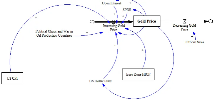
The objective of our forecasting model, gold price, is first set as a stock in the stock and flow diagram. The accumulation and reduction of gold price stock is a result of two major flows; rate of increasing price as the inflow and rate of decreasing price as the outflow. Six contributed factors to both flows are defined (see Fig. 2) via literature review in economics subject and interviewing with Thai practitioners in gold market.

Fig. 2. Factors affecting the gold price.

gold price or the one negatively relating to increasing of gold price is (5) U.S. Dollar Index, the performance measure of U.S. Dollar against a basket of currencies. Because the world gold market now seems to be dominated by U.S. dollar bloc, appreciations or depreciations of that dollar usually effects on the price of gold. The dollar depreciation results in increasing gold price due to the fact that investor wants to lower their risk on exchange rate. Then, the only main factor for outflows or decreasing of gold price is (6) Official Sales from various countries and organizations around the world. Whenever, some world’s largest gold holders announce official gold sales, it will negatively impact demand in gold market and finally reduce the market price. At this point we have come up with the system dynamic model for gold price and its related major factors as shown in Fig. 2. However, because consumer price indexes, both the U.S. and Euro zone ones, are highly affected from fluctuation of crude oil price, we then have to extend our model in more detail on the underlying factors associate with such indexes particularly the oil price. Added oil price modelling is illustrated in Fig. 3.

Fig. 3. Factors affecting the oil price and the gold price.

Readers interested in elaboration process of oil price modelling are recommended to refer to the author’s previous publication [8]. In summary, two out of six factors from gold price model are found to have impact on the oil price (i.e., U.S. Dollar Index and Chaos/War Factor). Like gold price model, U.S. Dollar Index ties to oil price negatively. When the dollar falls, oil prices rise because investors are more likely to transfer their investments toward more on oil (and gold as described earlier). In terms of chaos factor, whenever there is war or political issues in oil production countries, it means there will be limitation or tension of oil supply. Thus the oil price will be increasing as a consequent. Such circumstances have been evidenced for long through many world crisis periods such as the Suez Crisis in 1956, the Arab-Israel War in 1973, the Iranian Revolution (Islamic Revolution) in 1978 and the Persian Gulf War in 1990 [9].

Euro Dollar. Because the euro makes up most of the U.S. Dollar Index, a change in Euro will eventually affect the U.S. dollar index. Specifically speaking, increasing in exchange rate (e.g., 1.4 Euro/$US to be 1.6 Euro/$US) means increasing in U.S. Dollar Index therefore positive relationship is assigned between Euro exchange rate and U.S. Dollar Index.

Then, there is also the relationship between the inflation rate and the exchange rate. Using the Absolute Purchasing Power Parity Theory, which states that a bundle of goods should cost the same in any country once the exchange rate is taken into account. The law of one price between these two currencies can be expressed mathematically as shown in Eq. (1).

Exchange Rate Euro Dollar = Euro Customer Price Index (Euro Zone HICP) (1)

US Customer Price Index (US CPI)

The formula above clearly explains two relationships in our model; the positive correlation between exchange rate and Euro Zone HICP as well as the negative correlation between exchange rate and US CPI. At this instant, our system dynamic model elaborates casual relationships among all major variables influencing gold and oil prices as well as the relationship between them. The only economic variable included at present is the Customer Price Index (CPI). Having its own fluctuation, it is thus necessary to detail more regarding underlying factors controlling the CPI to come up with the better forecasting model. As a measure of inflation, any factors influencing inflation are incorporated in to our model at this stage as variables affect the CPIs, both US and Euro Zone CPI. Inflation is basically the change in the level of prices over time. Two main causes of inflation are Demand-Pull and Cost-Push Inflation. Demand-pull inflation occurs when there is an increase in aggregate demand due to economic growth. In the other words, there is positive relationship exists between the GDP and the increasing of CPI. Then, we further our model to include variables utilized in GDP calculation. A common used method for GDP computation is the expenditure approach, which involves counting expenditures on goods and services by different groups in the economy such as (11) personal consumption expenditures (C), (12) gross private domestic investment (I), (13) government consumption expenditures and gross investment (G), (14) exports of goods and services (X) and (15) imports of goods and services (M). In the expenditure approach, GDP is expressed in term of the above variables using Eq. (2).

GDP = C + I+ G + X – M (2)

Fig. 4. System dynamic model for the gold price.

3.

Mathematical Model Formulation

3.1. Quantitative Data

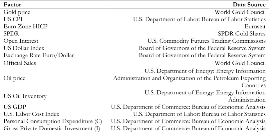
At this phase, it is necessary to identify all relationships shown in Fig. 4 mathematically in order to utilize the model for forecasting purpose. To perform this, we apply linear regression using least squares method. Historical data available to public are gathered from various data sources as listed in Table 1. Note that we used monthly historical data staring from year 2002 until 2009 to derive all relationships.

Table 1. Model variables and source of analysis data.

Factor Data Source

Gold price World Gold Council

US CPI U.S. Department of Labor: Bureau of Labor Statistics

Euro Zone HICP Eurostat

SPDR SPDR Gold Shares

Open Interest U.S. Commodity Futures Trading Commissions

US Dollar Index Board of Governors of the Federal Reserve System

Exchange Rate Euro/Dollar Board of Governors of the Federal Reserve System

Official Sales World Gold Council

Oil price Administration and Organization of the Petroleum Exporting U.S. Department of Energy: Energy Information Countries

US Oil Inventory U.S. Department of Energy: Energy Information _{Administration}

US GDP U.S. Department of Commerce: Bureau of Economic Analysis

U.S. Labor Cost Index U.S. Department of Labor: Bureau of Labor Statistics

Personal Consumption Expenditure (C) U.S. Department of Commerce: Bureau of Economic Analysis

Factor Data Source

Government Consumption

Expenditures and Gross Investment (G) U.S. Department of Commerce: Bureau of Economic Analysis

Exports of Goods and Services (X) U.S. Department of Commerce: Bureau of Economic Analysis

Imports of Goods and Services (M) U.S. Department of Commerce: Bureau of Economic Analysis

Euro Zone GDP Eurostat

Euro Zone Labor Cost Index Eurostat

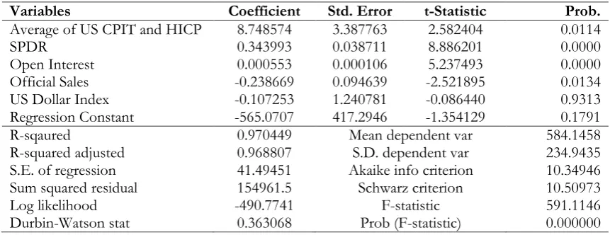
For example, the program run result for the relationship between Gold Price as a dependent variable and five independent variables (i.e., average of US CPI and Euro Zone HICP, SPDR, Open Interest, US Dollar Index, and Official Sales) is shown in Table 2.

Table 2. Linear regression analysis of the gold price model.

Variables Coefficient Std. Error t-Statistic Prob.

Average of US CPIT and HICP SPDR

Open Interest Official Sales US Dollar Index Regression Constant 8.748574 0.343993 0.000553 -0.238669 -0.107253 -565.0707 3.387763 0.038711 0.000106 0.094639 1.240781 417.2946 2.582404 8.886201 5.237493 -2.521895 -0.086440 -1.354129 0.0114 0.0000 0.0000 0.0134 0.9313 0.1791 R-sqaured R-squared adjusted S.E. of regression Sum squared residual Log likelihood Durbin-Watson stat 0.970449 0.968807 41.49451 154961.5 -490.7741 0.363068

Mean dependent var S.D. dependent var Akaike info criterion

Schwarz criterion F-statistic Prob (F-statistic) 584.1458 234.9435 10.34946 10.50973 591.1146 0.000000

Thus, equation used to predict gold price in our model is shown in Eq. (3). Note that this equation is used only under no chaos factor.

Gold Price t = 9 (average of US CPI t-1 and HICP t-1) + 0.35 SPDR t-1 + 0.00055 (3)

Open Interest t-1 – 0.239 Official Sales t-1 – 0.107 US Dollar Index t-1 -565

Utilizing similar methods repeatedly, we are able to describe all related regression relationships. These derived relationships sufficiently connect fifteen variables shown in the model whereas the qualitative factor (i.e., political chaos and war factor) will require different process discussed in the following section.

3.2. Qualitative Data

Because there is also qualitative variable in our model, transformation of this data into quantitative value is necessary. Through extensive reviewing of gold price and oil price historical data, we found that whenever there is economic crisis, the prices would soar up over our forecasting speculation. Average of 4% up for the gold price and 5% up for the oil price are found. Therefore, to quantify the effect of this variable, we have set up additional parameter to both gold and oil price formulas. This added parameter is calculating from percentage of price change multiplied by the price from its previous time period. Then, another regression analysis was performed to eventually gain Eq. (4) used to predict gold price under situation when there is chaos factor. In terms of inputting data for our dynamic model, the chaos variable holds default setting at “0” meaning that there is no political chaos or war in oil production countries. However, when it occurs, manually alters the variable input to be “1” is needed to trigger additional adjustment to eventually heighten up the gold price.

Gold Price t = 3.95 (average of US CPI t-1 and HICP t-1) + 0.17 SPDR t-1 + 0.00034 (4)

Open Interest t-1 -0.0823 Official Sales t-1 – 2.28 US Dollar Index t-1

Additionally, because the chaos and war factor is also expected to affect oil price, our model thus includes two separate equations used in the prediction of oil price under with and without chaos situation.

3.3. Example of Gold Price Prediction using System Dynamics Model

As mentioned in the earlier section, our model predicts gold price utilizing interactions among predefined variables. Basically, values from the prior time period will feedback and being inputs for predicting the other variables in the subsequent time. Also, there are variables which are not calculated results of the regression equations but rather being added into model under appropriate time. These variables include chaos factor and official sales.

For example, to predict gold price for January 2010 (t1), our model requires inputs including some

actual values from December 2009 (t0) (i.e., those in steps 1-5) and calculation results from regression

equations (i.e., those in steps 6-9) as shown in Table 3.

Table 3. Variable values for gold price prediction (t0).

Step Factors Values Status / Regression Equation

1 Gold Price (t0) 1,087.50 Initial Value

2 US CPI (t0) 110.56 Initial Value

3 Euro Zone HICP (t0) 108.91 Initial Value

4 Chaos Factor (t0) 0 Constant

5 Official Sales (t0) 0 Constant

6 SPDR (t0) 1,112.59 1.5 Gold Price (t0) – 518.66

7 Open Interest (t0) 496,208 363 Gold Price (t0) + 101445

8 Exchange Rate Euro/Dollar (t0) 0.734 5.74 (Euro Zone HICP (t0)/ US CPI (t0)) – 4.92

9 US Dollar Index (t0) 77.19 82.2001 Exchange Rate Euro/Dollar (t_{– 0.002 Gold Price (t} 0)

0) + 19

Then, gold price (t1) is calculated by inputting all values shown in Table 3 into Eq. (3)

Gold Price (t1)= 9 (110.56+108.91)/2 + 0.35(1,112.59) + 0.00055(496,208) - 0.239(0)

– 0.107(77.19) -565

= 1,076.68

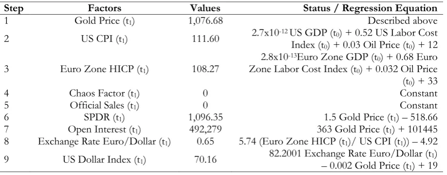
Once the model acquires this calculated gold price (t1), all other variables in which gold price is an

independent variable will further calculated. Example results for t1 are shown in Table 4.

Table 4. Variable values for gold price prediction (t1).

Step Factors Values Status / Regression Equation

1 Gold Price (t1) 1,076.68 Described above

2 US CPI (t1) 111.60 2.7x10

-12 _{US GDP (t0) + 0.52 US Labor Cost}

Index (t0) + 0.03 Oil Price (t0) + 12

3 Euro Zone HICP (t1) 108.27

2.8x10-13_{Euro Zone GDP (t0) + 0.68 Euro}

Zone Labor Cost Index (t0) + 0.032 Oil Price

(t0) + 33

4 Chaos Factor (t1) 0 Constant

5 Official Sales (t1) 0 Constant

6 SPDR (t1) 1,096.35 1.5 Gold Price (t1) – 518.66

7 Open Interest (t1) 492,279 363 Gold Price (t1) + 101445

8 Exchange Rate Euro/Dollar (t1) 0.65 5.74 (Euro Zone HICP (t1)/ US CPI (t1)) – 4.92

9 US Dollar Index (t1) 70.16 82.2001 Exchange Rate Euro/Dollar (t_{– 0.002 Gold Price (t} 1)

Note that in order to acquire values for independent variables related with US CPI and Euro Zone HICP, some other initial inputs are required at period t0.

4.

Model Evaluation

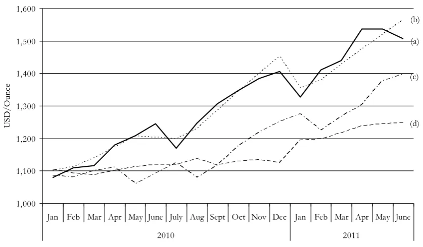
For evaluation purpose, we inputted initial value for all variables using actual available data of December 2009 (i.e., gold price, oil price, US CPI, Euro zone HICP, gross private domestic investment, exports and imports of goods) except the official sales and US oil inventory which manually input are required monthly. Then, the model will forecast gold price from January 2010 until the predefined end time. Note that we use Vensim system dynamic program as the tool for calculating all interaction effects defined earlier. Our basic assumption is that the model can forecast gold price until there is change in the qualitative variable or economic chaos factor. Therefore, as in year 2010, the first chaos happened around the end of February when there was a massive earthquake in Chile and Curacao and the productions of two oil refineries were halted due to the damages, the first estimation of year 2010 is run through only January and February. Then, to estimate price in March 2010 onward, we need to manually input the actual February data and change the Political chaos or war variable to “1” to illustrate that the event occurs so that the system will determine the 4% and 5% of growing up gold and oil price respectively. We hold these initial values and predict gold price from March 2010 until June 2010. Later, in June and July 2010, there was an excess oil supply that made the oil price lower than the predicted value. So another adjustment was made, by using actual data in June 2010 as initial input and switching “Political chaos or war in oil production countries” to be “0” and this setting can estimate the following two months until flooding problem happened in Pakistan during August 2010. Thus, another adjusting was made by using actual August 2010 data as the inputs combined with value “1” of chaos factor, here we can estimate gold price from September until December 2010. Note that various chaos factors actually happen along this time period, starting from an insurrection in France in September and October. Petrol shortages were spreading across the country as all 12 oil refineries had joined a continuous strike. Some 2,700 of France’s 12,600 petrol stations had completely run out of supplies. Also, there was crisis in Tunisia along this time. These chaos has relief around December 2010, thus we have again put December data and switch “0” to estimate January and February 2011 gold prices. Lastly, starting from the end of February 2011 until June 2011, there was agitation in Egypt and Libya, thus initial data of February 2011 was used and chaos factor is set at “1” to estimate gold price until June 2011. Following data input methodology discussed in this section, Fig. 5 compares the actual gold price data from January 2010 to June 2011 with the expected (forecast) counterparts.

Fig. 5. Comparison of (a) actual gold price data and the forecast gold price data using (b) system dynamics, (c) holt-winter exponential smoothing, and (d) box-jenkins.

1,000 1,100 1,200 1,300 1,400 1,500 1,600

Jan Feb Mar Apr May June July Aug Sept Oct Nov Dec Jan Feb Mar Apr May June

2010 2011

U

SD

/O

un

ce

(a) (b)

(c)

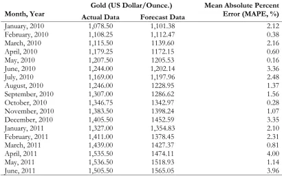
Our system dynamic model developed in this paper can forecast gold price with the average of 2% mean absolute percent error (MAPE). This prediction error is much lower than approximately 9% error found with Holt-Winter Exponential Smoothing and 11% error using Box-Jenkins Method. Approaches and formulas used in the later two methods are described in [12] and [13] respectively. Major underlying reasons for better prediction is expected to be the result of having ability to take into account of qualitative factors particularly political chaos and economic crisis events into system dynamic forecasting model. At the same time, system dynamic scheme allows possibility for incorporation of interaction and feedback effects among all related variables rather than relying solely on historical data as found in Time series. Table 3 shows the monthly percentage error from our model calculation.

Table 5. Results of monthly percentage of error.

Month, Year _{Actual Data} Gold (US Dollar/Ounce.) _{Forecast Data} Mean Absolute Percent Error (MAPE, %)

January, 2010 1,078.50 1,101.38 2.12

February, 2010 1,108.25 1,112.47 0.38

March, 2010 1,115.50 1139.60 2.16

April, 2010 1,179.25 1172.15 0.60

May, 2010 1,207.50 1205.53 0.16

June, 2010 1,244.00 1,202.14 3.36

July, 2010 1,169.00 1,197.96 2.48

August, 2010 1,246.00 1228.95 1.37

September, 2010 1,307.00 1286.62 1.56

October, 2010 1,346.75 1342.97 0.28

November, 2010 1,383.50 1398.24 1.07

December, 2010 1,405.50 1452.59 3.35

January, 2011 1,327.00 1,354.83 2.10

February, 2011 1,411.00 1378.45 2.31

March, 2011 1,439.00 1427.37 0.81

April, 2011 1,535.50 1474.11 4.00

May, 2011 1,536.50 1518.93 1.14

June, 2011 1,505.50 1565.05 3.96

5.

Limitation and Future Study

Although system dynamics model is shown to be a valid forecasting approach as discussed in the previous section, updating of data input approximately every three months is somewhat necessary. Without continually trace on chaos factor, the percentage error of gold price forecasting from January 2010 to June 2011 is nearly 9% in average with the maximum of 18% error around the last three months. Therefore, to effectively utilize our forecasting approach and maintain a low level of error term, the analyst shall follow closely to the world’s economics and political issues. This might be easier said than done because to trigger the chaos factor is relied entirely on the analyst’s decision and past experience. The same limitation is also present when making decision on taken off this qualitative factor from the model.

Lastly, as we all know, gold price is not affected from only U.S. and European countries’ economics but also from all other major countries such as the BRIC (i.e., Brazil, Russia, China, and India). The authors have well recognized this fact but due to constraint in language translation as well as accessibility to those countries’ economics data, the studied model have not yet included data from such nations. We strongly believe that taking into account all major countries concurrently will result in even more accurate model. Particularly with the fact that China’s economy has roared over the last 10 years and correlation between China’s CPI and gold prices over this period is shown to be higher than that with the U.S. CPI [14]. Also, as this study is thefirst exercise of system dynamics applied to the field of forecasting, there is possibility to utilize the same approach toward prediction of other interests than gold (e.g., rubber price, rice price, and other precious metals’ prices).

References

[1] E. F. Wolstenholme, “Qualitative v. quantitative modelling: The evolving balance,” J Oper Res Soc, vol. 50, no. 4, pp. 422-428, 1999.

[2] J. W. Forrester, and L. A. Martin, “Beginner exercises,” MIT System Dynamics in Education Project,

MIT, Cambridge, MA, Technical Report, 1997.

[3] S. G. Bantz, and M. L. Deaton, “Understanding U.S. biodiesel industry growth using system dynamics,”

in IEEE Systems and Information Engineering Design Symposium, Charlottesville, VA, pp. 156-161, 2006.

[4] S. Albin, “Building a system dynamics model part 1: Conceptualization,” MIT System Dynamics in

Education Project, MIT, Cambridge, MA, Technical Report, 1997.

[5] System Dynamics Group, “Guided study program in system dynamics,” MIT, Cambridge, MA,

Technical Report, 1998.

[6] L. A. Sjaastad, and F. Scacciavillani, “The price of gold and the exchange rate,” J Int Money Financ, vol. 15, no. 6, pp. 879-897, 1996.

[7] M. Feldstein, “The effects of inflation on the prices of land and gold,” J Public Econ, pp. 309-317, 1981.

[8] P. Vannasetta, and W. Tharmmaphornphilas, “Oil price using system dynamics,” in Proceedings of the

2nd _{International Conference on Business and Economics, Lhasa, Tibet, 2011.}

[9] J. H. Davis, and R.. A. Aliaga-Diaz, “Oil, the economy, and the stock market [online],” 2008.

Available http://ssrn.com/abstract=1136524 or http://dx.doi.org/10.2139/ssrn.1136524

[10] R. Pirog, “Oil industry profit review 2005,” CRS, Washington DC, Order Code RL33373, 2006.

[11] Thailand Securities Institute, in Economics 2nd ed., Bangkok, Thailand: The Stock Exchange of Thailand, 2005.

[12] T. Tanawut, and T. Keetashewa, “Forecasting system of gold bar price (in Thai).” Bachelor Thesis, Department of Computer Science, HCU, BKK, 2007.

[13] A. Mongkolkaset, “Analysis of influencing factors on gold price (in Thai).” Master Thesis,

Department of “Business Economics, UTCC, BKK, 2008.

[14] R. Cullen, “Do gold prices correlate with U.S. inflation? [online]” 2011. Available