Pattern vectors from algebraic graph theory

This is a repository copy of

Pattern vectors from algebraic graph theory

.

White Rose Research Online URL for this paper:

http://eprints.whiterose.ac.uk/1994/

Article:

Wilson, R C orcid.org/0000-0001-7265-3033, Hancock, E R

orcid.org/0000-0003-4496-2028 and Luo, B (2005) Pattern vectors from algebraic graph

theory. IEEE Transactions on Pattern Analysis and Machine Intelligence. pp. 1112-1124.

ISSN 0162-8828

https://doi.org/10.1109/TPAMI.2005.145

[email protected] https://eprints.whiterose.ac.uk/ Reuse

Items deposited in White Rose Research Online are protected by copyright, with all rights reserved unless indicated otherwise. They may be downloaded and/or printed for private study, or other acts as permitted by national copyright laws. The publisher or other rights holders may allow further reproduction and re-use of the full text version. This is indicated by the licence information on the White Rose Research Online record for the item.

Takedown

If you consider content in White Rose Research Online to be in breach of UK law, please notify us by

Pattern Vectors from Algebraic Graph Theory

Richard C. Wilson,

Member

,

IEEE Computer Society

, Edwin R. Hancock, and Bin Luo

Abstract—Graph structures have proven computationally cumbersome for pattern analysis. The reason for this is that, before graphs can be converted to pattern vectors, correspondences must be established between the nodes of structures which are potentially of different size. To overcome this problem, in this paper, we turn to the spectral decomposition of the Laplacian matrix. We show how the elements of the spectral matrix for the Laplacian can be used to construct symmetric polynomials that are permutation invariants. The coefficients of these polynomials can be used as graph features which can be encoded in a vectorial manner. We extend this representation to graphs in which there are unary attributes on the nodes and binary attributes on the edges by using the spectral decomposition of a Hermitian property matrix that can be viewed as a complex analogue of the Laplacian. To embed the graphs in a pattern space, we explore whether the vectors of invariants can be embedded in a low-dimensional space using a number of alternative strategies, including principal components analysis (PCA), multidimensional scaling (MDS), and locality preserving projection (LPP). Experimentally, we demonstrate that the embeddings result in well-defined graph clusters. Our experiments with the spectral representation involve both synthetic and real-world data. The experiments with synthetic data demonstrate that the distances between spectral feature vectors can be used to discriminate between graphs on the basis of their structure. The real-world experiments show that the method can be used to locate clusters of graphs.

Index Terms—Graph matching, graph features, spectral methods.

æ

1

I

NTRODUCTION

T

HEanalysis of relational patterns or graphs has proven to be considerably more elusive than the analysis of vectorial patterns. Relational patterns arise naturally in the representa-tion of data in which there is a structural arrangement and are encountered in computer vision, genomics, and network analysis. One of the challenges that arise in these domains is that of knowledge discovery from large graph data sets. The tools that are required in this endeavor are robust algorithms that can be used to organize, query, and navigate large sets of graphs. In particular, the graphs need to be embedded in a pattern space so that similar structures are close together and dissimilar ones are far apart. Moreover, if the graphs can be embedded on a manifold in a pattern space, then the modes of shape variation can be explored by traversing the manifold in a systematic way. The process of constructing low-dimen-sional spaces or manifolds is a routine procedure with pattern-vectors. A variety of well-established techniques, such as principal components analysis [12], multidimensional scaling [7], and independent components analysis, together with more recently developed ones, such as locally linear embed-ding [28], isomap [36], and the Laplacian eigenmap [2], exist for solving the problem. In addition to providing generic data analysis tools, these methods have been extensively exploited in computer vision to construct shape—spaces for 2D or 3D objects and, in particular, faces represented using coordinate and intensity data. Collectively, these methods

are sometimes referred to as manifold learning theory. However, there are few analogous methods which can be used to construct low-dimensional pattern spaces or mani-folds for sets of graphs.

There are two reasons why pattern-vectors are more easily manipulated than graphs. First, there is no natural ordering for the nodes in a graph, unlike the components of a vector. Hence, correspondences to a reference structure must be established as a prerequisite. The second problem is that the variation in the graphs of a particular class may manifest itself as subtle changes in structure, which may involve different numbers of nodes or different edge structure. Even if the nodes or the edges of a graph could be encoded in a vectorial manner, then the vectors would be of variable length. One way of circumventing these problems is to develop graph-clustering methods in which an explicit class archetype and correspondences with it are maintained [25], [31]. Graph clustering is an important process since it can be used to structure large databases of graphs [32] in a manner that renders retrieval efficient. One of the problems that hinders graph clustering is the need to define a class archetype that can capture both the salient structure of the class and the modes of variation contained within it. For instance, Munger et al. [22] have recently taken some important steps in this direction by developing a genetic algorithm for searching for median graphs. Variations in class structure can be captured and learned provided a suitable probability distribution can be defined over the nodes and edges of the archetype. For instance, the random graphs of Wong et al. [40] capture this distribution using a discretely defined probability distribu-tion and Bagdanov and Worring [1] have overcome some of the computational difficulties associated with this method by using continuous Gaussian distributions. There is a consider-able body of related literature in the graphical models community concerned with learning the structure of Baye-sian networks from data [11]. Moreover, in recent work, we have shown that, if reliable correspondence information is to hand, then the edge structure of the graph can be encoded as a . R.C. Wilson and E.R. Hancock are with the Department of Computer

Science, University of York, Heslington, York Y01 5DD, UK. E-mail: {wilson, erh}@cs.york.ac.uk.

. B. Luo is with the Key Lab of Intelligent Computing and Signal Processing of the Ministry of Education, Anhui University, Hefei 230039, P.R. China. E-mail: [email protected].

Manuscript received 3 Dec. 2003; revised 16 July 2004; accepted 1 Oct. 2004; published online 12 May 2005.

Recommended for acceptance by M. Basu.

For information on obtaining reprints of this article, please send e-mail to: [email protected] and reference IEEECS Log Number TPAMISI-0393-1203.

long-vector and embedded in a low-dimensional space using principal components analysis [20]. An alternative to using a probability distribution over a class archetype is to use pairwise clustering methods. Here, the starting point is a matrix of pairwise affinities between graphs. There are a variety of algorithms available for performing pairwise clustering, but one of the most popular approaches is to use spectral methods, which use the eigenvectors of an affinity matrix to define clusters [33], [13]. There are a number of examples of applying pairwise clustering methods to graph edit distances and similarity measures [19], [23].

However, one of the criticisms that can be aimed at these methods for learning the distribution of graphs is that they are, in a sense, brute force because of their need for correspondences either to establish an archetype or to compute graph similarity. For noisy graphs (those which are subject to structural differences), this problem is thought to be NP-hard. Although relatively robust approximate methods exist for computing correspondence [5], these can prove time consuming. In this paper, we are interested in the problem of constructing pattern vectors for graphs. These vectors represent the graph without the need to compute correspondences. These vectors are necessarily large, since they must represent the entire set of graphs of a particular size. For this reason, we are also interested in pattern spaces for families of graphs. In particular, we are interested in the problem of whether it is possible to construct a low-dimensional pattern space from our pattern vectors.

The adopted approach is based on spectral graph theory [6], [21], [3]. Although existing graph-spectral methods have proven effective for graph-matching and indexing [38], they have not made full use of the available spectral representa-tion and are restricted to the use of either the spectrum of eigenvalues or a single eigenvector.

1.1 Related Literature

Spectral graph theory is concerned with understanding how the structural properties of graphs can be characterized using the eigenvectors of the adjacency matrix or the closely related Laplacian matrix (the degree matrix minus the adjacency matrix). There are good introductory texts on the subject by Biggs [3] and Cvetkovic et al. [8]. Comprehensive reviews of recent progress in the field can be found in the research monograph of Chung [6] and the survey papers of Lovasc [17] and Mohar [21]. The subject has acquired considerable topicality in the computer science literature since spectral methods can be used to develop efficient methods for path planning and data clustering. In fact, the Googlebot search engine uses ideas derived from spectral graph theory. Techniques from spectral graph theory have been applied in a number of areas in computer vision, too, and have led to the development of algorithms for grouping and segmenta-tion [33], correspondence matching [38], [18], and shape indexing [34]. Among the first to apply spectral ideas to the grouping problem were Scott and Longuet-Higgins [30], who showed how to extract groups of points by relocating the eigenvectors of a point-proximity matrix. However, probably the best known work in this area is that of Shi and Malik [33], who showed how the Fiedler (second smallest) eigenvector of the Laplacian matrix could be used to locate groupings that optimize a normalized cut measure. In related work, both Perona and Freeman [24], and Sarkar and Boyer [29] have shown how the thresholded leading eigenvector of the weighted adjacency matrix can be used for grouping points

and line-segments. Robles-Kelly and Hancock [26] have developed a statistical variant of the method which avoids thresholding the leading eigenvector and instead employs the EM algorithm to iteratively locate clusters of objects.

The use of graph-spectral methods for correspondence matching has proven to be an altogether more elusive task. The idea underpinning spectral methods for correspondence analysis is to locate matches between nodes by comparing the eigenvectors of the adjacency matrix. However, although this method works well for graphs with the same number of nodes and small differences in edge structure, it does not work well when graphs of different size are being matched. The reason for this is that the eigenvectors of the adjacency matrix are unstable under changes in the size of the adjacency matrix. Turning to the literature, the algorithm of Umeyama [38] illustrates this point very clearly. The method commences by performing singular value decomposition on the adjacency matrices of the graphs under study. The permutation matrix which brings nodes of the graphs into correspondence is found by taking the sum of the outer products of the sets of corresponding singular vectors. The method cannot be operated when the adjacency matrices are of different size, i.e., the singular vectors are of different length. To overcome this problem, Luo and Hancock [18], have drawn on the apparatus of the EM algorithm and treat the correspondences as missing or hidden data. By introducing a correspondence probability matrix, they overcome problems associated with the different sizes of the adjacency matrices. An alternative solution to the problem of size difference is adopted by Kosinov and Caelli [16] who project the graph onto the eigenspace spanned by its leading eigenvectors. Provided that the eigenvectors are normalized, then the relative angles of the nodes are robust to size difference under the projection. In related work, Kesselman et al. have used a minimum distortion procedure to embed graphs in a low-dimensional space where correspondences can be located between groups of nodes [14]. Recent work by Robles-Kelly and Hancock [27] has shown how an eigenvector method can be used to sort the nodes of a graph into string order and how string matching methods can be used to overcome the size difference problem. Finally, Shokoufandeh et al. [34] have shown how to use the interleaving property of the eigenvalues to index shock trees.

1.2 Contribution

Size differences between graphs can be accommodated by padding the spectral matrix with trailing vectors of zeros.

The representation can be extended to attributed graphs using graph property matrices with complex entries instead of the real valued Laplacian. We show how weighted and attributed edges can be encoded by complex numbers with the weight as the magnitude or modulus and the attribute as the phase. If the property matrices are required to be Hermitian, then the eigenvalues are real and the eigenvectors are complex. The real and imaginary components of the eigenvectors can again be used to compute symmetric polynomials.

We explore how the spectral feature vectors may be used to construct pattern spaces for sets of graphs [14]. We investigate a number of different approaches. The first of these is to apply principal components analysis to the covariance matrix for the vectors. This locates a variance preserving embedding for the pattern vectors. The second approach is multidimensional scaling and this preserves the distance between vectors. The third approach is locally linear projection which aims to preserve both the variance of the data and the pattern of distances [10]. We demon-strate that this latter method gives the best graph-clusters.

The outline of this paper is as follows: Section 2 details our construction of the spectral matrix. In Section 3, we show how symmetric polynomials can be used to construct permutation invariants from the elements of the spectral matrix. Section 4 provides details of how the symmetric polynomials can be used to construct useful pattern vectors and how problems of variable node-set size can be accommodated. To accommodate attributes, in Section 5, we show how to extend the representation using complex numbers to construct a Hermitian property matrix. Section 6 briefly reviews how PCA, MDS, and locality preserving projection can be performed on the resulting pattern vectors. In Section 7, we present results on both synthetic and real-world data. Finally, Section 8 offers some conclu-sions and suggests directions for further investigation.

2

S

PECTRAL

G

RAPH

R

EPRESENTATION

Consider the undirected graphG ¼ ðV;E;WÞwith node-set

V ¼ f1; 2;. . .; ng, edge-set E ¼ fe1; e2;. . .; emg V V,

and weight functionW:E ! ð0;1. The adjacency matrixA

for the graphGis thennmatrix with elements

Aab¼ 1₀ if_otherwiseða; bÞ 2 E

:

In other words, the matrix represents the edge structure of the graph. Clearly since the graph is undirected, the matrixAis symmetric. If the graph edges are weighted, the adjacency matrix is defined to be

Aab¼ ₀Wða; bÞ if_otherwiseða; bÞ 2 E

:

The Laplacian of the graph is given byL_¼DA, whereD

is the diagonal node degree matrix whose elementsDaa¼

Pn

b¼1Aabare the number of edges which exit the individual

nodes. The Laplacian is more suitable for spectral analysis than the adjacency matrix since it is positive semidefinite.

In general, the task of comparing two such graphs,

G1 and G2, involves finding a correspondence mapping

between the nodes of the two graphs, f:_V1[$ V2[.

The recovery of the correspondence mapfcan be posed as that of minimizing an error criterion. The minimum value of the criterion can be taken as a measure of the similarity of the two graphs. The additional node “” represents a null match or dummy node. Extraneous or additional nodes are matched to the dummy node. A number of search and optimization methods have been developed to solve this problem [5], [9]. We may also consider the correspondence mapping problem as one of finding the permutation of nodes in the second graph which places them in the same order as that of the first graph. This permutation can be used to map the Laplacian matrix of the second graph onto that of the first. If the graphs are isomorphic, then this permutation matrix satisfies the

condition L1¼PL2PT. When the graphs are not

iso-morphic, then this condition no longer holds. However,

the Frobenius distance jjL1PL2PTjj between the

matrices can be used to gauge the degree of similarity between the two graphs. Spectral techniques have been used to solve this problem. For instance, working with adjacency matrices, Umeyama [38] seeks the

permutation matrix PU that minimizes the Frobenius

norm JðPUÞ ¼ jjPUA1PTUA2jj. The method performs

the singular value decompositions A1¼U11UT1 and

A2¼U22UT2, where theUs are orthogonal matrices and

the s are diagonal matrices. Once these factorizations

have been performed, the required permutation matrix is approximated by U2UT1.

In some applications, especially structural chemistry, eigenvalues have also been used to compare the structural similarity of different graphs. However, although the eigenvalue spectrum is a permutation invariant, it repre-sents only a fraction of the information residing in the eigensystem of the adjacency matrix.

Since the matrix L is positive semidefinite, it has

eigenvalues which are all either positive or zero. The spectral matrix is found by performing the eigenvector expansion for the Laplacian matrixL, i.e.,

L¼X

n i¼1

ieieTi;

wherei andei are then eigenvectors and eigenvalues of

the symmetric matrix L. The spectral matrix then has the scaled eigenvectors as columns and is given by

¼ ffiffiffiffiffi1

p

e1;

ffiffiffiffiffi 2

p

e2;. . .

ffiffiffiffiffi n

p

en

: ð1_Þ

The matrixis a complete representation of the graph in the sense that we can use it to reconstruct the original Laplacian matrix using the relationL_¼T.

The matrix is a unique representation of L iff all

3

N

ODE

P

ERMUTATIONS AND

I

NVARIANTS

The topology of a graph is invariant under permutations of the node labels. However, the adjacency matrix and, hence, the Laplacian matrix, is modified by the node order since the rows and columns are indexed by the node order. If we relabel the nodes, the Laplacian matrix undergoes a permutation of both rows and columns. Let the matrixPbe the permutation matrix representing the change in node order. The permuted matrix isL0¼PLPT. There is a family of Laplacian matrices which are can be transformed into one another using a permutation matrix. The spectral matrix is also modified by permutations, but the permutation only reorders the rows of the matrixTo show this, letLbe the Laplacian matrix of a graph G and let L0_¼PLPT be the Laplacian matrix obtained by relabeling the nodes using the permutationP. Further, letebe a normalized eigenvector of

Lwith associated eigenvalueand lete0_{¼Pe. With these}

ingredients, we have that

L0e0_¼PLPTPe_¼PLe_¼e0:

Hence,e0_{is an eigenvector ofL}0_{with associated eigenvalue.}

As a result, we can write the spectral matrix 0 of the

permuted Laplacian matrixL0¼00T as0¼P. Direct comparison of the spectral matrices for different graphs is, hence, not possible because of the unknown permutation.

The eigenvalues of the adjacency matrix have been used as a compact spectral representation for comparing graphs because they are not changed by the application of a permutation matrix. The eigenvalues can be recovered from the spectral matrix using the identity

j¼

Xn

i¼1

2_ij:

The expressionPn

i¼12ijis, in fact, asymmetric polynomialin

the components of eigenvectorei. A symmetric polynomial

is invariant under permutation of the variable indices. In this case, the polynomial is invariant under permutation of the row indexi.

In fact, the eigenvalue is just one example of a family of symmetric polynomials which can be defined on the components of the spectral matrix. However, there is a special set of these polynomials, referred to as theelementary symmetric polynomials(S) that form a basis set for symmetric polynomials. In other words, any symmetric polynomial can itself be expressed as a polynomial function of the elementary symmetric polynomials belonging to the setS.

We therefore turn our attention to the set of elementary symmetric polynomials. For a set of variablesfv1; v2. . .vng,

they can be defined as

S1ðv1;. . .vnÞ ¼P n i¼1

vi;

S2ðv1;. . .vnÞ ¼P n i¼1

Pn

j¼iþ1

vivj;

.. .

Srðv1;. . .vnÞ ¼ P i1<i2<...<ir

vi1vi2. . .vir;

.. .

Snðv1;. . .vnÞ ¼Q n i¼1

vi:

The power symmetric polynomial functions,

P1ðv1;. . .vnÞ ¼P n i¼1

vi;

P2ðv1;. . .vnÞ ¼P n i¼1

v2

i;

.. .

Prðv1;. . .vnÞ ¼P n i¼1

vr i;

.. .

Pnðv1;. . .vnÞ ¼P n i¼1

vn i;

also form a basis set over the set of symmetric polynomials. As a consequence, any function which is invariant to permuta-tion of the variable indices and that can be expanded as a Taylor series can be expressed in terms of one of these sets of polynomials. The two sets of polynomials are related to one another by the Newton-Girard formula:

Sr ¼ð

1_Þrþ1 r

Xr

k¼1

ð1ÞkþrPkSrk; ð2Þ

where we have used the shorthandSr for Srðv1;. . .: : ; vnÞ

andPrforPrðv1;. . .; vnÞ. As a consequence, the elementary

symmetric polynomials can be efficiently computed using the power symmetric polynomials.

In this paper, we intend to use the polynomials to construct invariants from the elements of the spectral matrix. The polynomials can provide spectral “features” which are invariant under node permutations of the nodes in a graph and utilize the full spectral matrix. These features are constructed as follows: Each column of the spectral matrix

forms the input to the set of spectral polynomials. For example, the columnf1;i;2;i;. . .;n;igproduces the

poly-nomials S1ð1;i;. . .;n;iÞ, S2ð1;i;. . .;n;iÞ;. . .; Snð1;i;. . .;

n;iÞ. The values of each of these polynomials is invariant to

the node order of the Laplacian. We can construct a set of

n2_{spectral features using thencolumns of the spectral matrix} in combination with thensymmetric polynomials.

Each set ofnfeatures for each spectral mode contains all the information about that mode up to a permutation of components. This means that it is possible to reconstruct the original components of the mode given the values of the features only. This is achieved using the relationship between the roots of a polynomial inxand the elementary symmetric polynomials. The polynomial

Y

i

ðxviÞ ¼0 ð3Þ

has rootsv1; v2;. . .; vn. Multiplying out (3) gives

xnS1xn1þS2xn2þ. . .þ ð1ÞnSn¼0; ð4Þ

where we have again used the shorthand Sr for

Srðv1;. . .: : ; vnÞ. By substituting the feature values into

4

P

ATTERN

V

ECTORS FROM

S

YMMETRIC

P

OLYNOMIALS

In this section, we detail how the symmetric polynomials can be used to construct graph feature vectors which can be used for the purposes of pattern analysis. There are two practical issues that need to be addressed. The first of these is how to deal with graphs which have node-sets of different size. The second is how to transform the vectors into an informative representation.

4.1 Graphs of Different Sizes

In order to accommodate graphs with different numbers of nodes, we need to be able to compare spectral representations of different sizes. This is achieved by expanding the

representation. Consider two graphs with m andn nodes,

respectively, wherem < n. If we addnmnodes with no connections to the smaller graph, we obtain two graphs of the same size. The edit cost in terms of edge insertions and deletions between these two graphs is identical to the original pair. The effect on the spectral representation is merely to add trailing zeros to each eigenvector and also additional zero

eigenmodes. As a consequence, the first m elementary

symmetric polynomials are unchanged and the subsequent

nmpolynomials are zero. The new representation in the symmetric polynomialsScan therefore be easily calculated. The corresponding power symmetric polynomials can be calculated using the Newton-Girard formula. This new representation can be directly compared with that for the larger graph.

4.2 Feature Distributions

While the elementary symmetric polynomials provide spectral features which are invariant to permutations, they are not suitable as a representation for gauging the difference between graphs. The distribution of Sr for large

ris highly non-Gaussian with a dominant tail because of the product terms appearing in the higher order polynomials. In order to make the distribution more tractable, it is convenient to take logarithms. If we wish to take logarithms, the conditionSr>08rmust hold. We therefore perform a

component transform and construct the following matrix from the symmetric polynomials

Fij¼signumSjð1;i;2;i;. . .;n;iÞ

ln 1þ jSjð1;i;2;i;. . .;n;iÞj

; ð5Þ

where 1in;1jn. The rows of this matrix are

stacked to form a long-vector

B¼ ðF1;1;. . .; F1;n; F2;1;. . .; F2;n;. . .; Fn;1;. . .; Fn;nÞT: ð6Þ

4.3 Complexity

The computational complexity of generating pattern vectors is governed by the eigendecomposition of the Laplacian matrix. This requires Oðn3

Þ operations, where n is the

number of vertices in the graph. Computation of the symmetric polynomials and subsequent feature representa-tions only requires Oðn2

Þ operations. These operations are effectively preprocessing of the graph structures. Matching of two graphs simply involves comparing two pattern vectors of lengthn2_{and, so, takesOðn}2_{Þoperations. Standard} inexact matching techniques are generally iterative and, for comparison, both the graduated assignment algorithm of

Gold and Rangarajan [9] and probabilistic relaxation [5] requireOðn4

Þoperations per iteration.

5

U

NARY AND

B

INARY

A

TTRIBUTES

Attributed graphs are an important class of representations and need to be accommodated in graph matching. Van Wyk and van Wyk [39] have suggested the use of an augmented matrix to capture additional measurement information. While it is possible to make use of a such an approach in conjunction with symmetric polynomials, another approach from the spectral theory of Hermitian matrices suggests itself. A Hermitian matrixHis a square matrix with complex elements that remains unchanged under the joint operation of transposition and complex conjugation of the elements (denoted by the dagger operatory), i.e.,Hy_¼H. Hermitian matrices can be viewed as the complex number counterpart of the symmetric matrix for real numbers. Each off-diagonal element is a complex number which has two components and can therefore represent a 2-component measurement vector on a graph edge. The on-diagonal elements are, necessarily, real quantities, so the node measurements are restricted to be scalar quantities.

There are some constraints on how the measurements may be represented in order to produce a positive semidefinite Hermitian matrix. Letfx1; x2;. . .; xng be a set of

measure-ments for the node-setV. Further, letfy1;2; y1;3;. . .; yn;ngbe the

set of measurements associated with the edges of the graph in addition to the graph weights. Each edge then has a pair of observations ðWa;b; ya;bÞ associated with it. There are a

number of ways in which the complex numberHa;b could

represent this information, for example, with the real part as

Wand the imaginary part asy. However, we would like our complex property matrix to reflect the Laplacian. As a result, the off-diagonal elements ofHare chosen to be

Ha;b¼ Wa;beiyab:

In other words, the connection weights are encoded by the magnitude of the complex numberHa;b and the additional

measurement by its phase. By using this encoding, the magnitude of the numbers is the same as in the original Laplacian matrix. Clearly, this encoding is most suitable when the measurements are angles. If the measurements are easily bounded, they can be mapped onto an angular interval and phase wrapping can be avoided. If the measurements are not easily bounded, then this encoding is not suitable.

The measurements must satisfy the conditions

ya;b< and ya;b¼ yb;a to produce a Hermitian matrix.

To ensure a positive definite matrix, we require

Haa>Pb6¼ajHabj. This condition is satisfied if

Haa¼xaþ

X

b6¼a

Wa;b

andxa0:

When defined in this way, the property matrix is a complex analogue of the weighted Laplacian for the graph.

For a Hermitian matrix, there is an orthogonal complete basis set of eigenvectors and eigenvalues obeying the

eigenvalue equation He¼e. In the Hermitian case,

the eigenvalues are real and the components of the

also a solution, i.e.,He¼e. In the real case, we choose

such thateis of unit length. In the complex case,itself may be complex and needs to determined by two constraints. We set the vector length tojeij ¼1and, in addition, we impose the

condition argPn

i¼1ei¼0, which specifies both real and

imaginary parts.

This representation can be extended further by using the four-component complex numbers known as quaternions. As with real and complex numbers, there is an appropriate eigendecomposition which allows the spectral matrix to be found. In this case, an edge weight and three additional binary measurements may be encoded on an edge. It is not possible to encode more than one unary measurement using this approach. However, for the experiments in this paper, we have concentrated on the complex representation.

When the eigenvectors are constructed in this way, the spectral matrix is found by performing the eigenvector expansion

H¼X

n i¼1

ieieyi;

whereiandeiare theneigenvectors and eigenvalues of the

Hermitian matrix H. We construct the complex spectral

matrix for the graphGusing the eigenvectors as columns, i.e.,

_¼ ffiffiffiffiffi1

p

e1;

ffiffiffiffiffi 2

p

e2;. . .

ffiffiffiffiffi n

p

en

: ð7_Þ

We can again reconstruct the original Hermitian property matrix using the relationH_¼y.

Since the components of the eigenvectors are complex numbers, therefore, each symmetric polynomial is complex. Hence, the symmetric polynomials must be evaluated with complex arithmetic and also evaluate to complex numbers. EachSr therefore has both real and imaginary components.

The real and imaginary components of the symmetric polynomials are interleaved and stacked to form a feature-vectorBfor the graph. This feature-vector is real.

6

G

RAPH

E

MBEDDING

M

ETHODS

We explore three different methods for embedding the graph feature vectors in a pattern space. Two of these are classical methods. Principal components analysis (PCA) finds the projection that accounts for the variance or scatter of the data. Multidimensional scaling (MDS), on the other hand, preserves the relative distances between objects. The remaining method is a newly reported one that offers a compromise between preserving variance and the relational arrangement of the data and is referred to as locality preserving projection [10].

In this paper, we are concerned with the set of graphs

G1;G2; : : ;Gk;. . .;GN. The kth graph is denoted by Gk¼

ðVk;EkÞand the associated vector of symmetric polynomials

is denoted byBk.

6.1 Principal Component Analysis

We commence by constructing the matrix X¼ ½B1BB

jB2BBj. . .jBk BBj. . .jBNBB, with the graph feature

vectors as columns. Here,BB is the mean feature vector for the data set. Next, we compute the covariance matrix for the elements of the feature vectors by taking the matrix

product C¼XXT. We extract the principal components

directions by performing the eigendecomposition C_¼

PN

i¼1liuiuTi on the covariance matrix C, where the li are

the eigenvalues and theui are the eigenvectors. We use the

firstsleading eigenvectors (2 or 3, in practice, for visualiza-tion purposes) to represent the graphs extracted from the images. The coordinate system of the eigenspace is spanned by thesorthogonal vectors U¼ ðu1;u2; : :;usÞ. The

indivi-dual graphs represented by the long vectors Bk; k¼

1;2;. . .; N can be projected onto this eigenspace using the formula y_k¼UTðBkBBÞ. Hence, each graphGk is

repre-sented by ans-componentvectorykin the eigenspace.

Linear discriminant analysis (LDA) is an extension of PCA to the multiclass problem. We commence by constructing separate data matrices X1;X2;. . .XNc for each of the Nc

classes. These may be used to compute the corresponding class covariance matrices Ci¼XiXTi. The average class

covariance matrix CC~_¼1

Nc

PNc

i¼1Ci is found. This matrix is

used as a sphering transform. We commence by computing the eigendecomposition

~ C

C¼X

N i¼1

liuiuTi ¼UUT;

where U is the matrix with the eigenvectors of CC~ as

columns and ¼diagðl1; l2; : : ; lnÞ is the diagonal

eigenva-lue matrix. The sphered representation of the data is

X0_¼1

2UTX. Standard PCA is then applied to the

resulting data matrixX0. The purpose of this technique is to find a linear projection which describes the class differences rather than the overall variance of the data.

6.2 Multidimensional Scaling

Multidimensional scaling (MDS) is a procedure which allows data specified in terms of a matrix of pairwise distances to be embedded in a Euclidean space. Here, we intend to use the method to embed the graphs extracted from different viewpoints in a low-dimensional space. To commence, we require pairwise distances between graphs. We do this by computing the norms between the spectral pattern vectors for the graphs. For the graphs indexedi1andi2, the distance is

di1;i2¼ ðBi1Bi2Þ

T

ðBi1Bi2Þ. The pairwise distancesdi1;i2

are used as the elements of anNNdissimilarity matrixR, whose elements are defined as follows:

Ri1;i2¼

di1;i2 ifi16¼i2 0 ifi1¼i2:

ð8Þ

In this paper, we use the classical multidimensional scaling method [7] to embed the graphs in a Euclidean space using the matrix of pairwise dissimilaritiesR. The first step of MDS is to calculate a matrixTwhose element with rowr

and column c is given by Trc¼ 12½d 2

rcdd^2r:dd^2:cþdd^2::,

where dd^r:¼N1

PN

c¼1drc is the average dissimilarity value

over therthrow,dd^:cis the dissimilarity average value over

the cth column and dd^::¼N12 PN

r¼1

PN

c¼1dr;c is the average

dissimilarity value over all rows and columns of the dissimilarity matrixR.

We subject the matrix T to an eigenvector analysis to obtain a matrix of embedding coordinatesY. If the rank ofT

is k; kN, then we will havek nonzero eigenvalues. We

arrange these k nonzero eigenvalues in descending

eigenvectors are denoted by ui, where li is the

ith eigenvalue. The embedding coordinate system for the

graphs is Y¼ ½ ffiffi

ð

p

l1Þu1;pffiffiffiffil2u2;. . .;pffiffiffiffilsus. For the graph

indexedj, the embedded vector of coordinates is a row of matrixY, soyj¼ ðYj;1; Yj;2;. . .; Yj;sÞT.

6.3 Locality Preserving Projection

Our next pattern space embedding method is He and Niyogi’s Locality Preserving Projections(LPP) [10]. LPP is a linear dimensionality reduction method which attempts to project high-dimensional data to a low-dimensional mani-fold, while preserving the neighborhood structure of the data set. The method is relatively insensitive to outliers and noise. This is an important feature in our graph clustering task since the outliers are usually introduced by imperfect segmentation processes. The linearity of the method makes it computationally efficient.

The graph feature vectors are used as the columns of a data-matrixX¼ ðB1jB2j. . .jBNÞ. The relational structure of

the data is represented by a proximity weight matrixWwith elementsWi1;i2¼exp½kdi1;i2, wherekis a constant. IfQis

the diagonal degree matrix with the row weights Qk;k¼

PN

j¼1Wk;j as elements, then the relational structure of the

data is represented using the Laplacian matrixJ¼QW. The idea behind LPP is to analyze the structure of the weighted covariance matrixXWXT. The optimal projection of the data is found by solving the generalized eigenvector problem

XJXTu¼lXQXTu: ð9_Þ

We project the data onto the space spanned by the eigenvectors corresponding to the s smallest eigenvalues. LetU¼ ðu1;u2;. . .;usÞbe the matrix with the corresponding

eigenvectors as columns, then projection of thekth feature vector isyk¼UTBk.

7

E

XPERIMENTS

There are three aspects to the experimental evaluation of the techniques reported in this paper. We commence with a study on synthetic data aimed at evaluating the ability of the spectral features to distinguish between graphs under controlled structural error. The second part of the study focuses on real-world data and assesses whether the spectral feature vectors can be embedded in a pattern space that

reveals cluster-structure. Here, we explore the two different applications of view-based polyhedral object recognition and shock graph recognition. The latter application focuses on the use of the complex variant of the property matrix.

7.1 Synthetic Data

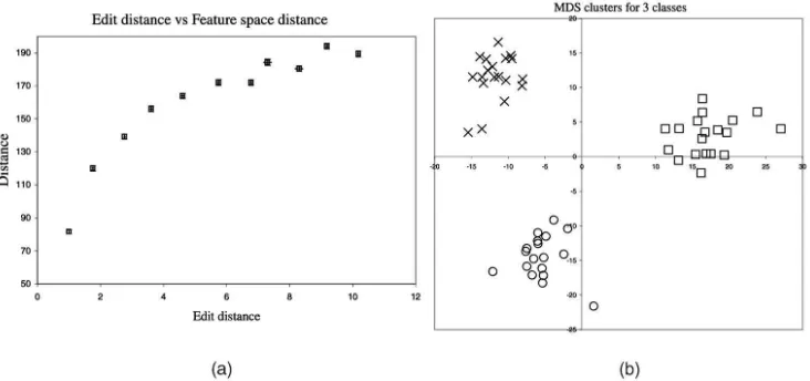
We commence by examining the ability of the spectral feature set and distance measure to separate both structurally related and structurally unrelated graphs. This study utilizes random graphs which consist of 30 nodes and 140 edges. The edges are generated by connecting random pairs of nodes. From each seed graph constructed in this way, we generate structurally related graphs by applying random edit operations to simulate the effect of noise. The structural variants are generated from a seed graph by either deleting an edge or inserting a new random edge. Each of these operations is assigned unit cost and, therefore, a graph with a deleted edge has unit edit distance to the original seed graph. In Fig. 1a, we have plotted the distribution of feature vector distancedi1;i2¼ ðBi1Bi2Þ

T

ðBi1Bi2Þfor two sets of

graphs. The leftmost curve shows the distribution of distances when we take individual seed graphs and remove a single edge at random. The rightmost curve is the distribution of distance obtained when we compare the distinct seed graphs. In the case of the random edge-edits, the modal distance between feature vectors is much less than that for the structurally distinct seed graphs. Hence, the distance between feature vectors appears to provide scope for distinguishing between distinct graphs when there are small variations in edge structure due to noise.

The results presented in Table 1 take this study one step further and demonstrate the performance under different levels of corruption. Here, we have computed the confusion probability, i.e., the overlap between distribution of feature-vector distance for the edited graphs and the seed graphs, as a

Fig. 1. (a) Distributions of distance to edited graphs and (b) eigenvectors.

TABLE 1

[image:8.612.93.480.73.229.2]

function of the number of randomly deleted edges. The confusion probability increases with increasing edit distance. In Fig. 1b, we investigate the effect of the different eigenmodes used in computing symmetric polynomials. We again compute the confusion probability due to the overlap of the two distance distributions. Here, we confine our attention to the removal of a single edge. Only one eigenvector is used in the distance measure. Eigenvector-n denotes the eigen-vector with thenthlargest eigenvalue. The plot demonstrates that the leading and the last few eigenvectors give the lowest confusion probabilities and are, hence, the most important in differentiating graph structure.

At first sight, this suggests that only a few of the eigenvectors need be used to characterize the graph. However, as Table 2 reveals, this is only the case for small edit distances. As the edit distance increases, then more of the eigenvectors become important.

In Fig. 2a, we plot the distance in feature space, i.e.,di1;i2¼

ðBi1Bi2Þ

T

ðBi1Bi2Þ as a function of the graph edit

distance. Although the relationship is not linear, it is monotonic and approximately linear for small edit distances. Hence, the distance between the feature vectors does reflect in a direct way the changes in structure of the graphs.

To provide an illustration, we have created three clusters of graphs from three seed or reference graphs by perturbing them by edit operations. The distances between the feature-vectors for these graphs are then used to embed the graphs in a two-dimensional space using multidimensional scaling. The procedure is as follows: Three seed graphs are generated

at random. These seed graphs are used to generate samples by deleting an edge at random from the graph. The distance matrix is then constructed, which has elements di1;i2, the

distance between graphs i1 and i2. Finally, the MDS

technique is used to visualize the distribution of graphs in a two-dimensional space. The results are shown in Fig. 2b. The graphs form good clusters and are well-separated from one another.

To take this study on synthetic data one step further, we have performed a classification experiment. We have generated 100 graphs of 25 nodes each. For each graph, the edge-structure is randomly generated. Associated with each edge is a weight randomly and uniformly drawn from the interval ½0;1. We have investigated the effect of adding random noise to the edge-weights. The weight noise is drawn from a Gaussian distribution of zero mean and known standard deviation.

We have investigated the effect of this noise on three different vector representations of the weighted graphs. The first of these is a vector with the first four polynomial features as components. The second is a vector whose components are the bin-contents of the normalized edge-weight histogram. Here, the edge weights are allocated to eight uniformly spaced bins. The final vector has the leading four eigenvalues of the Laplacian matrix as components. We have computed the distances between the feature vectors for the uncorrupted and noise corrupted graphs. To compute a classification error rate, we have recorded the fraction of times that the uncorrupted graphs do not have the smallest distance to the corresponding noise corrupted graph. In Fig. 3, we show the error-rate as a function of the edge-weight noise standard deviation. The main features to note from this plot are that the lowest error rate is returned by the polynomial features and the highest error rate results from the use of the edge-weight histogram.

7.2 View-Based Object Recognition

[image:9.612.48.259.83.211.2]

Our first real-world experimental vehicle is provided by 2D views of 3D objects. We have collected sequences of views for three toy houses. For each object, the image sequences are obtained under slowly varying changes in viewer direction. From each image in each view sequence, we extract corner features. We use the extracted corner points to construct Delaunay graphs. In our experiments, we use three different sequences. Each sequence contains images with equally spaced viewing directions. In Fig. 4, TABLE 2

Confusion Probabilities of Different Eigenvector Sets and Edit Distances

[image:9.612.101.467.574.746.2]

we show examples of the raw image data and the associated graphs for the three toy houses which we refer to as CMU/ VASC, MOVI, and Swiss Chalet.

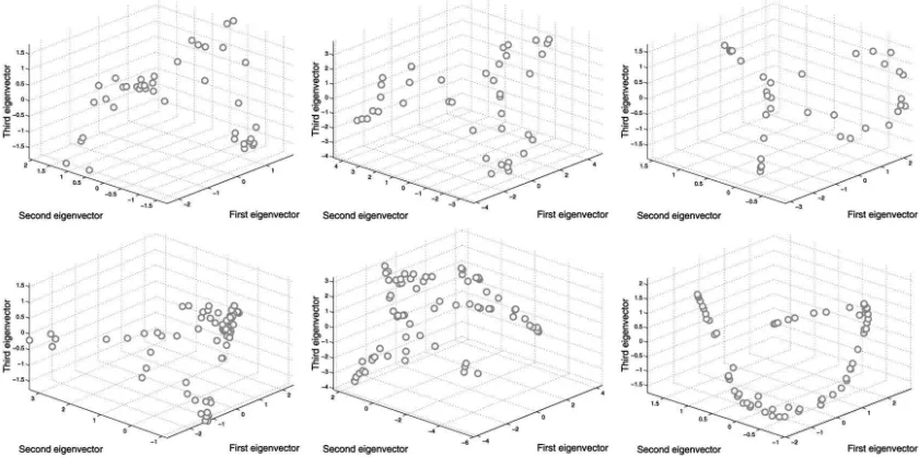
In Fig. 5, we compare the results obtained with the different embedding strategies and the different graph features. In Column 1, we show the results obtained when PCA is used, Column 2 when MDS is used, and Column 3 when LPP is used. The top row shows the results obtained using a standard spectral feature, namely, the spectrum ordered eigenvalues of the Laplacian, i.e.,Bk¼ ðk1; k2;. . .Þ

T

. The second row shows the results obtained when the symmetric polynomials are computed using the spectral matrix for the Laplacian. The different image sequences are displayed in various shades of gray and black.

There are a number of conclusions that can be drawn from this plot. First, the most distinct clusters are produced when either MDS or LPP are used. Second, the best spectral features seem to be the symmetric polynomials computed from the Laplacian spectral matrix. To display the cluster-structure obtained, in Fig. 6, we visualize the results obtained using LPP and the Laplacian polynomials by placing thumbnails of the original images in the space

spanned by the leading two eigenvectors. The different objects form well-separated and compact clusters.

To take this study further, we investigate the effects of applying the embedding methods to two of the sequences separately. Fig. 7 shows the results obtained with the Laplacian polynomials for MOVI and Chalet sequences. Column 1 is for PCA, Column 2 is for MDS, and Column 3 is for LPP. In the case of both image sequences, LPP results in a smooth trajectory as the different views in the sequence are traversed.

7.3 Shock Graphs

[image:10.612.296.535.70.212.2]

The final example focuses on the use of the complex property matrix representation and is furnished by shock trees which are a compact representation of curved boundary shape. There are a number of ways in which a shape graph can be computed [15], [35]. One of the most effective recent methods has been to use the Hamilton-Jacobi equations from classical mechanics to solve the eikonal equation for inward boundary motion [35]. The skeleton is the set of singularities in the boundary motion where opposing fronts collide and these can be characterized as locations where the divergence of the

[image:10.612.66.241.72.219.2]

Fig. 3. Classification error rates.

Fig. 4. Example images from the CMU, MOVI, and chalet sequences and their corresponding graphs.

[image:10.612.73.502.519.729.2]

distance map to the boundary is nonzero. Once detected, then the skeleton can be converted into a tree. There are several ways in which this can be affected. For instance, Kimia et al. use the branches and junctions of the skeleton as the nodes and edges of a tree [15]. Siddiqi et al. use the time of formation of singularities under the eikonal equation to order the points on the skeleton [35]. According to this representation, the root of the tree is located at the deepest point within the shape, i.e., the final skeleton point to be formed and the terminal nodes are the closest to the boundary. Once the tree is to hand, then it may be attributed with a number of properties of the boundaries. These might include the radius of the bitangent circle or the rate of change of skeleton length with boundary length. The tree may also be attributed with shock labels. These capture the differential structure of the boundary since they describe whether the radius of the bitangent circle is constant, increasing, decreasing, locally minimum, or locally maximum. The labels hence indicate whether the boundary is of constant width, tapering-out, tapering-in, locally con-stricted, or locally bulging.

7.3.1 Tree Attributes

Before processing, the shapes are firstly normalized in area and aligned along the axis of largest moment. After performing these transforms, the distances and angles associated with the different shapes can be directly compared and can therefore be used as attributes.

To abstract the shape skeleton using a tree, we place a node at each junction point in the skeleton. The edges of the tree represent the existence of a connecting skeletal branch between pairs of junctions. The nodes of the tree are characterized using the radiusrðaÞof the smallest bitangent circle from the junction to the boundary. Hence, for the node a, xa¼rðaÞ. The edges are characterized by two

measurements. For the edgeða; bÞ, the first of these,ya;bis the

angle between the nodesaandb, i.e.,ya;b¼ða; bÞ. Since most

skeleton branches are relatively straight, this is an approx-imation to the angle of the corresponding skeletal branch. Furthermore, since ða; bÞ< and ða; bÞ ¼ ðb; aÞ, the measurement is already suitable for use in the Hermitian property matrix.

In order to compute edge weights, we note that the importance of a skeletal branch may be determined by the rate of change of boundary lengthlwith skeleton lengths

[37], which we denote bydl=ds. This quantity is related to the rate of change of the bitangent circle radius along the skeleton, i.e.,dr=ds, by the formula

dl ds¼

ffiffiffiffiffiffiffiffiffiffiffiffiffiffiffiffiffiffiffiffiffiffi 1 dr

ds 2 s

:

The edge weightWa;bis given by the average value ofdl=ds

along the relevant skeletal branch.

It must be noted that the tree representation adopted here is relatively simplistic and more sophisticated alternatives exist elsewhere in the literature [15], [35]. It must be stressed that our main aim here is to furnish a simple attributed tree representation on which to test our spectral analysis.

[image:11.612.37.267.69.243.2]

It is a well-known fact that trees tend to be cospectral [4] which, as noted in Section 3, could be problematic for the spectral representation. However, because we are using

Fig. 6. LPP space clustering using the graph polynomials.

[image:11.612.71.491.536.745.2]

attributed trees, any ambiguity is removed by the measure-ment information.

7.3.2 Experiments with Shock Trees

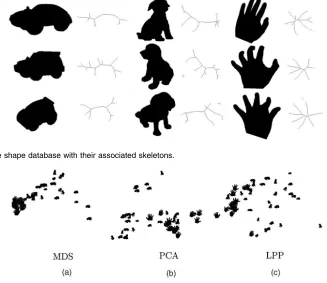
Our experiments are performed using a database of 42 binary shapes. Each binary shape is extracted from a 2D view of a 3D object. There are three classes in the database and, for each object, there are a number of views acquired from different viewing directions and a number of different examples of the class. We extract the skeleton from each binary shape and attribute the resulting tree in the manner outlined in Section 7.3.1. Fig. 8 shows some examples of the types of shape present in the database along with their skeletons.

[image:12.612.117.444.75.358.2]

We commence by showing some results for the three shapes shown in Fig. 8. The objects studied are a hand, some puppies, and some cars. The dog and car shapes consist of a number of different objects and different views of each object. The hand category contains different hand configurations. We apply the three embedding strategies outlined in Section 6 to the vectors of permutation invariants extracted from the Hermitian variant of the Laplacian. We commence in Fig. 9a by showing the result of applying the MDS procedure to the three shape categories. The “hand” shapes form a compact cluster in the MDS space. There are other local clusters consisting of three or four members of the remaining two classes. This reflects the fact that, while the hand shapes have very similar shock graphs, the remaining two categories have rather variable shock graphs because of the different objects. Fig. 9b shows the result of using PCA. Here, the distribu-tions of shapes are much less compact. While a distinct cluster of hand shapes still occurs, they are generally more dispersed over the feature space. There are some distinct clusters of the car shape, but the distributions overlap more in the PCA projection when compared to the MDS space.

Fig. 9c shows the result of the LPP procedure on the data set. The results are similar to the PCA method.

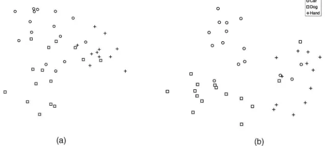
One of the motivations for the work presented here was the potential ambiguities that are encountered when using the spectral features of trees. To demonstrate the effect of using attributed trees rather than simply weighting the edges, we have compared the LDA projections using both types of data. Fig. 10 illustrates the result of this compar-ison. Fig. 10b shows the result obtained using the symmetric polynomials from the eigenvectors of the

Laplacian matrix L_¼DW, associated with the edge

weight matrix. Fig. 10a shows the result of using the using the Hermitian property matrix. The Hermitian property matrix for the attributed trees produces a better class separation than the Laplacian matrix for the weighted trees. The separation can be measured by the Fisher discriminant between the classes, which is the squared distance between class centers divided by the variance along the line joining the centers. For the Hermitian property matrix, the separations are 1.12 for the car/dog classes, 0.97 for the car/hand, and 0.92 for the dog/hand. For the weighted matrix, the separations are 0.77 for the car/dog, 1.02 for the car/hand, and 0.88 for the dog/hand.

8

C

ONCLUSIONS

In this paper, we have shown how graphs can be converted into pattern vectors by utilizing the spectral decomposition of the Laplacian matrix and basis sets of symmetric polynomials. These feature vectors are complete, unique, and continuous. However, and most important of all, they are permutation invariants. We investigate how to embed the vectors in a pattern space, suitable for clustering the graphs. Here, we explore a number of alternatives including

Fig. 8. Examples from the shape database with their associated skeletons.

[image:12.612.125.436.76.220.2]

PCA, MDS, and LPP. In an experimental study, we show that the feature vectors derived from the symmetric polynomials of the Laplacian spectral decomposition yield good clusters when MDS or LPP are used.

There are clearly a number of ways in which the work presented in this paper can be developed. For instance, since the representation based on the symmetric polynomials is complete, they may form the means by which a generative model of variations in graph structure can be developed. This model could be learned in the space spanned by the permutation invariants and the mean graph and its modes of variation reconstructed by inverting the system of equations associated with the symmetric polynomials.

A

CKNOWLEDGMENTS

Bin Luo is partially supported by the National Natural Science Foundation of China (No. 60375010).

R

EFERENCES

[1] A.D. Bagdanov and M. Worring, “First Order Gaussian Graphs for Efficient Structure Classification,” Pattern Recogntion, vol. 36, pp. 1311-1324, 2003.

[2] M. Belkin and P. Niyogi, “Laplacian Eigenmaps for Dimension-ality Reduction and Data Representation,” Neural Computation,

vol. 15, no. 6, pp. 1373-1396, 2003.

[3] N. Biggs,Algebraic Graph Theory.Cambridge Univ. Press, 1993.

[4] P. Botti and R. Morris, “Almost All Trees Share a Complete Set of Inmanantal Polynomials,” J. Graph Theory,vol. 17, pp. 467-476, 1993.

[5] W.J. Christmas, J. Kittler, and M. Petrou, “Structural Matching in Computer Vision Using Probabilistic Relaxation,” IEEE Trans. Pattern Analysis and Machine Intelligence,vol. 17, pp. 749-764, 1995.

[6] F.R.K. Chung, “Spectral Graph Theory,”Am. Math. Soc. Edition.,

CBMS series 92, 1997.

[7] T. Cox and M. Cox, Multidimensional Scaling. Chapman-Hall, 1994.

[8] D. Cvetkovic, P. Rowlinson, and S. Simic,Eigenspaces of Graphs.

Cambridge Univ. Press, 1997.

[9] S. Gold and A. Rangarajan, “A Graduated Assignment Algorithm for Graph Matching,” IEEE Trans. Pattern Analysis and Machine Intelligence,vol. 18, pp. 377-388, 1996.

[10] X. He and P. Niyogi, “Locality Preserving Projections,”Advances in Neural Information Processing Systems 16,MIT Press, 2003.

[11] D. Heckerman, D. Geiger, and D.M. Chickering, “Learning Bayesian Networks: The Combination of Knowledge and Statis-tical Data,”Machine Learning,vol. 20, pp. 197-243, 1995.

[12] I.T. Jolliffe,Principal Components Analysis.Springer-Verlag, 1986.

[13] R. Kannan et al., “On Clusterings: Good, Bad and Spectral,”Proc. 41st Symp. Foundation of Computer Science,pp. 367-377, 2000.

[14] Y. Kesselman, A. Shokoufandeh, M. Demerici, and S. Dickinson, “Many-to-Many Graph Matching via Metric Embedding,”Proc. IEEE Conf. Computer Vision and Pattern Recognition,pp. 850-857, 2003.

[15] B.B. Kimia, A.R. Tannenbaum, and S.W. Zucker, “Shapes, Shocks, and Deformations I. The Components of 2-Dimensional Shape and the Reaction-Diffusion Space,”Int’l J. Computer Vision, vol. 15, pp. 189-224, 1995.

[16] S. Kosinov and T. Caelli, “Inexact Multisubgraph Matching Using Graph Eigenspace and Clustering Models,”Proc. Joint IAPR Int’l Workshops Structural, Syntactic, and Statistical Pattern Recognition, SSPR 2002 and SPR 2002,pp. 133-142, 2002.

[17] L. Lovasz, “Random Walks on Graphs: A Survey,” Bolyai Soc. Math. Studies,vol. 2, pp. 1-46, 1993.

[18] B. Luo and E.R. Hancock, “Structural Matching Using the EM Algorithm and Singular Value Decomposition,”IEEE Trans. Pattern Analysis and Machine Intelligence,vol. 23, pp. 1120-1136, 2001.

[19] B. Luo, A. Torsello, A. Robles-Kelly, R.C. Wilson, and E.R. Hancock, ”A Probabilistic Framework for Graph Clustering,”Proc. IEEE Conf. Computer Vision and Pattern Recognition,pp. 912-919, 2001.

[20] B. Luo, R.C. Wilson, and E.R. Hancock, “Eigenspaces for Graphs,”

Int’l J. Image and Graphics,vol. 2, pp. 247-268, 2002.

[21] B. Mohar, “Laplace Eigenvalues of Graphs—A Survey,”Discrete Math.,vol. 109, pp. 171-183, 1992.

[22] A. Munger, H. Bunke, and X. Jiang, “Combinatorial Search vs. Genetic Algorithms: A Case Study Based on the Generalized Median Graph Problem,” Pattern Recognition Letters, vol. 20, pp. 1271-1279, 1999.

[23] M. Pavan and M. Pelillo, “Dominant Sets and Hierarchical Clustering,”Proc. Ninth IEEE Int’l Conf. Computer Vision, vol. I, pp. 362-369, 2003.

[24] P. Perona and W.T. Freeman, “A Factorization Approach to Grouping,”Proc. European Conf. Computer Vision,pp. 655-670, 1998.

[25] S. Rizzi, “Genetic Operators for Hierarchical Graph Clustering,”

Pattern Recognition Letters,vol. 19, pp. 1293-1300, 1998.

[26] A. Robles-Kelly and E.R. Hancock, “An Expectation-Maximisation Framework for Segmentation and Grouping,” Image and Vision Computing,vol. 20, pp. 725-738, 2002.

[27] A. Robles-Kelly and E.R. Hancock, “Edit Distance from Graph Spectra,”Proc. Ninth IEEE Int’l Conf. Computer Vision,vol. I, pp. 127-135, 2003.

[28] S. Roweis and L. Saul, “Non-Linear Dimensionality Reduction by Locally Linear Embedding,”Science,vol. 299, pp. 2323-2326, 2002.

[29] S. Sarkar and K.L. Boyer, “Quantitative Measures of Change Based on Feature Organization: Eigenvalues and Eigenvectors,”Computer Vision and Image Understanding,vol. 71, pp. 110-136, 1998.

[30] G.L. Scott and H.C. Longuet-Higgins, “Feature Grouping by Relocalisation of Eigenvectors of the Proximity Matrix,” Proc. British Machine Vision Conf.,pp. 103-108, 1990.

[31] J. Segen, “Learning Graph Models of Shape,”Proc. Fifth Int’l Conf. Machine Learning,J. Laird, ed., pp. 29-25, 1988.

[32] K. Sengupta and K.L. Boyer, “Organizing Large Structural Modelbases,”IEEE Trans. Pattern Analysis and Machine Intelligence,

[image:13.612.122.444.76.219.2]

vol. 17, 1995.

[33] J. Shi and J. Malik, “Normalized Cuts and Image Segmentation,”

IEEE Trans. Pattern Analysis and Machine Intelligence, vol. 22, pp. 888-905, 2000.

[34] A. Shokoufandeh, S. Dickinson, K. Siddiqi, and S. Zucker, “Indexing Using a Spectral Coding of Topological Structure,”Proc. IEEE Conf. Computer Vision and Pattern Recognition,pp. 491-497, 1999.

[35] K. Siddiqi, A. Shokoufandeh, S.J. Dickinson, and S.W. Zucker, “Shock Graphs and Shape Matching,” Int’l J. Computer Vision,

vol. 35, pp. 13-32, 1999.

[36] J.B. Tenenbaum, V.D. Silva, and J.C. Langford, “A Global Geometric Framework for Non-Linear Dimensionality Reduc-tion,”Science,vol. 290, pp. 586-591, 2000.

[37] A. Torsello and E.R. Hancock, “A Skeletal Measure of 2D Shape Similarity,”Proc. Fourth Int’l Workshop Visual Form,pp. 594-605, 2001.

[38] S. Umeyama, “An Eigen Decomposition Approach to Weighted Graph Matching Problems,” IEEE Trans. Pattern Analysis and Machine Intelligence,vol. 10, pp. 695-703, 1988.

[39] B.J. van Wyk and M.A. van Wyk, “Kronecker Product Graph Matching,”Pattern Recognition,vol. 39, no. 9, pp. 2019-2030, 2003.

[40] A.K.C. Wong, J. Constant, and M.L. You, “Random Graphs,”

Syntactic and Structural Pattern Recognition,World Scientific, 1990.

Richard C. Wilsonreceived the BA degree in physics from the University of Oxford in 1992. In 1996, he completed the PhD degree at the University of York in the area of pattern recognition. From 1996 to 1998, he worked as a research associate at the University of York. After a period of postdoctoral research, he was awarded an Advanced Research Fellowship in 1998. In 2003, he took up a lecturing post and he is now a reader in the Department of Computer Science at the University of York. He has published more than 100 papers in journals, edited books, and refereed conferences. He received an outstanding paper award in the 1997 Pattern Recognition Society awards and has won the best paper prize in ACCV 2002. He is currently an associate editor of the journal Pattern Recognition. His research interests are in statistical and structural pattern recognition, graph methods for computer vision, high-level vision, and scene understanding. He is a member of the IEEE Computer Society.

Edwin R. Hancock studied physics as an undergraduate at the University of Durham and graduated with honors in 1977. He remained at Durham to complete the PhD degree in the area of high-energy physics in 1981. Following this, he worked for 10 years as a researcher in the fields of high-energy nuclear physics and pattern recognition at the Rutherford-Appleton Labora-tory (now the Central Research LaboraLabora-tory of the Research Councils). In 1991, he moved to the University of York as a lecturer in the Department of Computer Science. He was promoted to senior lecturer in 1997 and to reader in 1998. In 1998, he was appointed to a chair in computer vision. Professor Hancock now leads a group of some 15 faculty, research staff, and PhD students working in the areas of computer vision and pattern recognition. His main research interests are in the use of optimization and probabilistic methods for high and intermediate level vision. He is also interested in the methodology of structural and statistical pattern recognition. He is currently working on graph-matching, shape-from-X, image databases, and statistical learning theory. He has published more than 90 journal papers and 350 refereed conference publications. He was awarded the Pattern Recognition Society medal in 1991 and an outstanding paper award in 1997 by the journalPattern Recognition. In 1998, he became a fellow of the International Association for Pattern Recognition. He has been a member of the editorial boards of the journalsIEEE Transactions on Pattern Analysis and Machine Intelli-genceand Pattern Recognition. He has also been a guest editor for special editions of the journalsImage and Vision ComputingandPattern Recognition.

Bin Luoreceived the BEng degree in electro-nics and the MEng degree in computer science from Anhui university of China in 1984 and 1991, respectively. From 1996 to 1997, he worked as a British Council visiting scholar at the University of York under the Sino-British Friendship Scho-larship Scheme (SBFSS). In 2002, he was awarded the PhD degree in computer science from the University of York, United Kingdom. He is at present a professor at Anhui University of China. He has published more than 60 papers in journals, edited books, and refereed conferences. His current research interests include graph spectral analysis, large image database retrieval, image and graph matching, statistical pattern recognition, and image feature extraction.