Random coeffcient models for complex longitudinal data

(1)

RANDOM COEFFICIENT MODELS FOR

COMPLEX LONGITUDINAL DATA

Darren Kidney

A Thesis Submitted for the Degree of PhD at the

University of St Andrews

2014

Full metadata for this item is available in Research@StAndrews:FullText

at:

http://research-repository.st-andrews.ac.uk/

Please use this identifier to cite or link to this item: http://hdl.handle.net/10023/6386

This item is protected by original copyright

(2)

Random coefficient models for

complex longitudinal data

Darren Kidney

Thesis submitted for the degree of

DOCTOR OF PHILOSOPHY

in the School of Mathematics and Statistics,

UNIVERSITY OF ST ANDREWS.

(3)

(4)

Declarations

1. Candidate’s declarations:

I, Darren Kidney, hereby certify that this thesis, which is approximately 30,000

words in length, has been written by me, that it is the record of work carried out

by me and that it has not been submitted in any previous application for a higher

degree.

I was admitted as a research student in September 2009 and as a candidate for the

degree of PhD in September 2010; the higher study for which this is a record was

carried out in the University of St Andrews between 2009 and 2014.

Date: signature of candidate:

2. Supervisor’s declarations:

I hereby certify that the candidate has fulfilled the conditions of the Resolution and

Regulations appropriate for the degree of PhD in the University of St Andrews and

that the candidate is qualified to submit this thesis in application for that degree.

Date: signature of supervisor:

3. Permission for electronic publication:

In submitting this thesis to the University of St Andrews I understand that I am

giv-ing permission for it to be made available for use in accordance with the regulations

of the University Library for the time being in force, subject to any copyright vested

in the work not being affected thereby. I also understand that the title and the

(5)

to any bona fide library or research worker, that my thesis will be electronically

accessible for personal or research use unless exempt by award of an embargo as

requested below, and that the library has the right to migrate my thesis into new

electronic forms as required to ensure continued access to the thesis. I have obtained

any third-party copyright permissions that may be required in order to allow such

access and migration, or have requested the appropriate embargo below.

The following is an agreed request by candidate and supervisor regarding the

elec-tronic publication of this thesis:

PRINTED COPY

Embargo on all of print copy for a period of 1 year on the following ground(s):

Publication would preclude future publication.

ELECTRONIC COPY

Embargo on all of electronic copy for a period of 1 year on the following ground(s):

Publication would preclude future publication.

Date: signature of candidate:

(6)

Abstract

Longitudinal data are common in biological research. However real data sets vary

considerably in terms of their structure and complexity and present many challenges

for statistical modelling. This thesis proposes a series of methods using random

coef-ficients for modelling two broad types of longitudinal response: normally distributed

measurements and binary recapture data.

Biased inference can occur in linear mixed-effects modelling if subjects are drawn

from a number of unknown sub-populations, or if the residual covariance is poorly

specified. To address some of the shortcomings of previous approaches in terms of

model selection and flexibility, this thesis presents methods for: (i) determining the

presence of latent grouping structures using a two-step approach, involving regression

splines for modelling functional random effects and mixture modelling of the fitted

random effects; and (ii) flexible of modelling of the residual covariance matrix using

regression splines to specify smooth and potentially non-monotonic variance and

correlation functions.

Spatially explicit capture-recapture methods for estimating the density of animal

populations have shown a rapid increase in popularity over recent years. However,

further refinements to existing theory and fitting software are required to apply

these methods in many situations. This thesis presents: (i) an analysis of recapture

data from an acoustic survey of gibbons using supplementary data in the form of

estimated angles to detections, (ii) the development of a multi-occasion likelihood

including a model for stochastic availability using a partially observed random

ef-fect (interpreted in terms of calling behaviour in the case of gibbons), and (iii) an

analysis of recapture data from a population of radio-tagged skates using a

condi-tional likelihood that allows the density of animal activity centres to be modelled as

(7)

(8)

Acknowledgements

Thanks to my supervisors, Monique MacKenzie and Carl Donovan, for their

guid-ance, support and considerable patience over the past four years. Thanks also to

David Borchers whose collaboration was crucial to the work in Chapters 5, 6 and 7

and who always made time for our many invaluable discussions.

The gibbon survey data in Chapter 5 were provided by Dr Ben Rawson whose

expert knowledge was vital to the applications in Chapters 5 and 6. Cecilia Pinto

also provided the skates data set used in Chapter 7 and made numerous visits from

Aberdeen to discuss data and analysis issues.

It would not have been possible to complete this thesis without the understanding

and generosity of my friends and family, to each of whom I owe an enormous debt of

gratitude: Jon Fraser and Paolo Pizzola, long-suffering house-mates, for their

toler-ance and camaraderie; Dad, Catharene, Sophie, Matthew, Cheryl, George, Isaac and

Florence for being constant sources of comfort, encouragement and entertainment;

and Alice, without whose unfailing support my sanity would have vanished a long

(9)

(10)

Introduction

1.1 General background

Longitudinal data are common in many areas of biological research and consist of

measurements of variables taken repeatedly over time on each of a set of

obser-vational units or ‘subjects’ (McCulloch, 2008; Diggle et al., 2013). Studies which

give rise to such data are often observational, making it difficult to either control

or observe the full range of variables which may affect a given response. Statistical

models for longitudinal data therefore need to cope with both known and unknown

sources of variability due to observed and hidden covariates.

The sources of variability in longitudinal data can be divided into two main types:

(i) Between-subject variability

This is typically described in statistical models using subject-level random

variables, commonly referred to as random effects1_{. While} _fixed _{effects are}

unknown constants that need to be estimated from the data, models using

ran-dom effects require estimation of the parameters which determine the shape of

their distributions rather than estimating them directly. The random

effects-based approach therefore enables inferences to be made about the population

from which the subjects were sampled while offering a more parsimonious

so-1_{More generally, where data exhibit a hierarchical clustering structure, random effects can be}

(17)

lution than treating the random effects as a series of fixed parameters. One

disadvantage of the random effects approach however is that models must be

expressed in marginal form which requires integration over all possible values

of the random effects. This makes them less tractable theoretically.

(ii) Within-subject variability

This relates to the variability at the level of the measurements themselves with

respect to their expected value, and is typically dealt with by assuming a joint

distribution for the measurement, conditional on the values of the random

and fixed effects. In models for normally distributed data, the within-subject

variability can be represented explicitly by associating a random error term

with each measurement, representing the difference between the measurement

and its expected value at the subject level. The joint distribution for the errors

is often assumed to be multivariate normal and can be modelled independently

of the expected values (in practice, inference is made on the distribution of

the residuals, which are the differences between the measurements and their

predicted values).

In the context of this thesis, random effects and error terms are taken as examples

ofrandom coefficients – i.e. terms whose values are not observed directly but which

are assumed to follow a given distribution.

The focus of this thesis is on the development of new methods within two distinct

modelling frameworks – linear mixed-effects models2 _{and spatially explicit}

capture-recapture – each of which use random coefficients to model longitudinal data.

1.1.1 Linear mixed-effects models

Linear mixed-effects (LME) models for normal longitudinal data (Laird and Ware,

1982; Ware, 1985) are widely used for investigating the changes over time of response

(18)

subject) where each series can be visualised as a curve orprofile. Considered in this

way, the fixed effects component of an LME model for longitudinal data is used to

describe the shape of the mean profile for a sample of subjects, while the random

effects describe the differences between the subject-specific profiles and the mean

profile.

A key advantage of LME models when compared with fitting separate regression

models for each subject, is that they allow strength to be borrowed across subjects

in the estimation of subject-specific profiles. Consequently LME models have the

potential to provide a more parsimonious description of the data and are better

able to handle missing values. LME models also explicitly partition the

within-and between-subject variance, through the use of separate covariance matrices for

the errors and random effects, which enables a detailed description of the overall

dependence structure in the data. When interest lies in making inference on the

shape of subject-specific profiles, as opposed to the overall mean for example, these

details are necessary.

Appropriate partitioning of variability is therefore key to obtaining sensible results

from LME models. However, two sources of difficulty in this regard are (i) the

pres-ence of unobserved grouping structures in the data and (ii) inadequate modelling

of the covariance matrices. Hidden grouping structures may exist as a result of the

data being collected from unidentified sub-populations of subjects. If subjects from

different sub-populations exhibit systematic differences in their mean profile shape,

then inferences on the overall mean profile could be meaningless and the

distribu-tion of the random effects is also likely to be misspecified. This misspecificadistribu-tion may

also cause bias in the estimation of subject-specific profiles (Verbeke and Lesaffre,

1996). Specification of the covariance matrix for the errors (or rather the

residu-als) also needs to be carefully considered in order to avoid biased inference for the

fixed effects. However, currently available methods for modelling residual covariance

structures are fairly limited and may not be flexible enough to model many of the

(19)

1.1.2 Spatially Explicit Capture-Recapture

Capture-recapture (CR) studies aim to estimate the abundance of animal

popula-tions. They involve the collection of longitudinal data on detected animals (the

‘subjects’) in the form of capture histories across a series of trapping occasions. CR

studies have traditionally relied on the use of physical traps which detain captured

animals for the remainder of the trapping occasion3_{. However, the advent of}

prox-imity detectors such as microphones and camera traps, which allow detections for

the same animal to be made at more than one detector on a given occasion (since

the detected animals are not physically detained), has enabled abundance estimates

to be obtained from single-occasion recapture data.

The main disadvantage of traditional models for CR data is their inability to

esti-mate population density, which is a more useful currency than abundance for making

comparisons between different regions. The reason for this is that these models

ig-nore the information contained in the spatial location of capture events (assuming

that the locations of detectors are known) and are therefore unable to provide

infer-ence on the effective size of the sampled area. Spatially explicit capture-recapture

(SECR) methods have been developed to address this issue (Efford, 2004; Borchers

and Efford, 2008; Royle and Young, 2008). These models allow direct estimation of

animal density by modelling the recapture data jointly with the unknown ‘locations’

(see Section 2.4.2) of the detected animals and treating the locations as random

effects. The sub-model for the recapture data in SECR also uses a detection

func-tion to describe the relafunc-tionship between detecfunc-tion probability and distance from

detector, thereby accounting for heterogeneity in capture probabilities due to

differ-ences in animal location, which is known to cause biased inference if left unmodelled

(Borchers and Efford, 2008).

SECR models have been used to estimate population density for a variety of species,

3_{These are divided into ‘single-catch’ traps, which can capture a maximum of one individual}

(20)

including horned lizards from visual trapping studies (Royle and Young, 2008),

minke whales using bottom-mounted hydrophones (Marques et al., 2010) and tigers

from camera traps arrays (Royle et al., 2009a,b). Recent developments have also

allowed the incorporation of supplementary data containing additional information

on animal location – e.g. in the form of received signal strengths, signal arrival

times, and estimated angles or distances to detected animals – in order to produce

more precise density estimates (Dawson and Efford, 2009; Borchers et al., 2014).

However, despite a substantial increase in the uptake of these methods over the past

few years, SECR is still in a relatively early stage of development and modifications

to the general theory are required for many specific applications. Currently available

procedures for fitting SECR models are also fairly limited and a greater degree of

investment is required in terms of software development to enable practitioners to

fully utilise these methods.

1.2 Thesis outline

Chapter 2 introduces the basic form of the likelihoods for linear mixed-effects models

(assuming normally distributed data) and spatially explicit capture-recapture, in

addition to key formulae and notation which are referred to in subsequent chapters.

Chapter 3 presents a procedure for exploring potential sub-populations in normally

distributed longitudinal data. The procedure consists of two steps: (i) an initial

LME modelling step usingB-spline design matrices in which model selection is used

to find a model that adequately describes the variation in shapes of the underlying

subject-specific profiles; followed by (ii) a clustering step in which the random effects

of the preferred model are clustered via mixture modelling. The approach aims to

address some of the drawbacks of previous methods for which model selection is

more problematic and consequently often neglected. The procedure is tested by

simulation and applied to a set of gene expression data which has been analysed in

(21)

Chapter 4 describes a method which uses B-splines to construct smooth variance

and correlation functions to address some of the limitations of existing tools for

modelling residual covariance matrices in models for normal longitudinal data. Using

a combination of non-standard link functions and a stabilised numerical optimisation

method the fitting procedure is able to converge on fitted functions which generate

viable covariance matrices. This modelling approach is able to fit smooth correlation

functions which can take negative values – a facility that is lacking in currently

available software. The methodology is first implemented in the context of a general

linear model (i.e. with no random effects) and then in the context of an LME model.

The method is examined in each case through the use of a simulation studies.

In Chapter 5 the focus of the thesis shifts to SECR models. Chapter 5 presents an

adaptation of the general SECR likelihood that permits the inclusion of

supplemen-tary information on animal location. In this case a model for estimated bearings is

formulated and applied to a pre-existing single-occasion data set from an acoustic

survey of gibbons to estimate the density of calling groups. In order to inform future

monitoring strategies, the performance of the model and survey design, in terms of

the precision of the density estimator, are investigated by simulation in comparison

with a selection of alternative designs.

Chapter 6 extends the model used in Chapter 5 for application to multi-occasion

gibbon survey data. Whilst general SECR models for multi-occasion data already

exist, they only offer a partial solution in the case of gibbons since they assume

that all animals are available for detection during each sampling occasion. However

gibbon groups do not call every day and may therefore be unavailable for detection

during a given sampling occasion. This behaviour is modelled by introducing a

random effect for availability which enables the density of groups, as opposed to

calling groups, to be estimated. Estimator properties from this extended form of

the SECR likelihood are tested via simulation.

(22)

form of the SECR likelihood4 _{which allows various components of the SECR model}

– namely the density surface, the detection function parameters and the

availabil-ity parameter introduced in Chapter 6 – to be modelled using linear combinations

of covariates. The covariates for each component were allowed to vary according to

animal-level variables (e.g. body size) and occasion-level variables (e.g. time).

Addi-tionally the density surface was allowed to vary with spatially referenced covariates.

Allowing the density surface to change with time also required a novel

reformula-tion of the SECR likelihood allowing animal locareformula-tions to change between occasions.

A formulation of the resulting model for situations where the entire population is

observed is tested using a simulation study and applied to a data set collected on a

population of radio-tagged skates.

Finally, Chapter 8 provides an overall summary of the methods presented in this

thesis and discusses ideas for future extensions and improvements.

(23)

(24)

Chapter 2

Review of methods

2.1 Introduction

This Chapter introduces some of the statistical theory on which the subsequent

Chapters rely. It is divided into three main parts: Section 2.2 introduces

regres-sion splines, with particular reference to B-splines (Chapters 3 and 4); Section 2.3

describes the basic theory of linear mixed-effects models (Chapters 3 and 4); and

Section 2.4 provides an overview of spatially explicit capture-recapture (Chapters 5,

6 and 7).

2.2 Regression splines

Regression splines1 provide a convenient way of modelling monotonic and non-monotonic relationships within the framework of linear models2_{. The general}

defi-nition of a regression spline is as follows,

p X

j=1

Bj(xi)βj, (2.1)

where xi is the ith measurement of a continuous covariate (i = 1, ...n), the Bj are

a set of pbasis functions (collectively referred to as a basis) and the βj are a series

1_{I.e. splines with no smoothness penalty.}

2_{‘Linear’ in this context refers to the manner in which terms are combined – namely as weighted}

(25)

of p coefficients which scale the values of the basis functions. The basis functions

of a spline are locally defined using the support of the explanatory variable – i.e.

they are non-zero over a subset of the values ofx (in contrast to simple polynomial

functions which are globally defined). Equation 2.1 can be represented using matrix

algebra as,

B(x)β=Xβ, (2.2)

where x is an n-vector of covariate values, B(x) = X is an n by p matrix whose

columns contain the values of the p basis functions, each of which are evaluated at

x, and where β is a p-vector of basis function coefficients.

2.2.1 B

-splines

The B-spline basis (De Boor, 1978) is a popular choice for constructing regression

splines. The basis functions of aB-spline are specified in terms of the degree (1 =

linear, 2 = quadratic, 3 = cubic, etc.) and the number and placement of theknots,

which determine the regions of x where the basis functions have non-zero values.

The knots are divided into two types: (i) boundary knots, which are placed at the

boundaries of the x values; and (ii) internal knots, which are placed between the

boundaries of the x values. The number of internal knots and the degree of the

B-spline basis determine the number of basis functions (for a B-spline that includes

an intercept, the number of basis functions is equal to the number of internal knots

plus the degree plus 1). The number of basis functions is also referred to as the

degrees of freedom of the basis.

The mathematical definition ofB-spline basis functions is based on a recursive

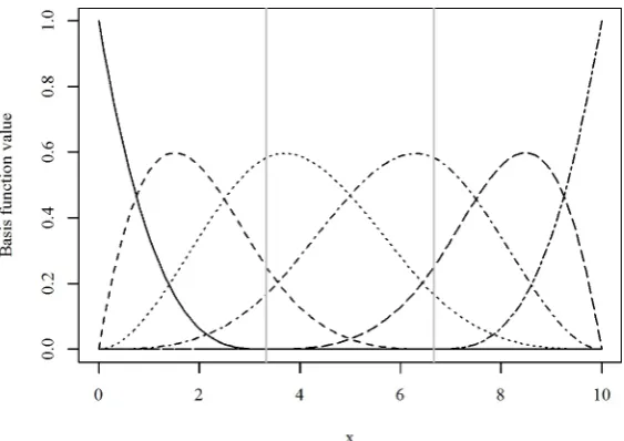
equa-tion and is not given here. However, they are easy to construct in R, for example using thebsfunction in thesplineslibrary (R Core Team, 2013). Figure 2.1 shows the unscaled basis function values for a degree 3B-spline with 6 degrees of freedom

(26)

[image:26.595.181.463.97.296.2]

Figure 2.1: Example B-spline basis with 6 degrees of freedom. Black lines show the individual basis functions and vertical grey lines show locations of the two internal knots

2.3 Linear mixed-effects models

This section summarises some of the basic theory of linear mixed effects models for

normal data, assuming normal random effects. The material in this section is largely

taken from Pinheiro and Bates (2000) and Verbeke and Molenberghs (2000).

2.3.1 Notation

M the number of subjects

i denotes the ith subject (i= 1, ..., M)

ni the number of response values for subject i

p the number of fixed effects

q the number of random effects

y_i a vector of response values (length ni)

Xi a design matrix for the fixed effects (ni rows by p columns)

Zi a design matrix for the random effects (ni rows by q columns)

β a vector fixed effect parameters (length p)

(27)

i a vector of error terms (length ni)

G the covariance matrix for the random effects (q rows by q columns)

Ri the covariance matrix for the errors (ni rows by ni columns)

Σi the covariance matrix for the response data (ni rows by ni columns)

θ a vector of all model parameters (incl. those for the covariance matrices)

2.3.2 Conditional model

The standard formulation of the linear mixed-effects model can be written as follows,

y_i =Xiβ+Zibi+i, (2.3)

where,

bi ∼M V N(0,G), i ∼M V N(0,Ri), (2.4)

and wherebi and i are independent and G and Ri must be positive definite.

The fact that both bi and i follow independent multivariate normal distributions

implies that the distribution for y_i, conditional on bi, will also be multivariate

normal,

y_i |bi ∼M V N(Xiβ+Zibi, Ri). (2.5)

2.3.3 Marginal model

Since the random effects,bi, are unobserved it is necessary to work with the marginal

density function of y_i. This is obtained by defining the joint density of y_i and bi

and integrating overbi,

f(y_i) =

Z

(28)

which implies the following marginal distribution,

y_i ∼M V N(Xiβ, Σi), (2.7)

where,

Σi =ZiGZTi +Ri. (2.8)

This shows that the covariance structure in the marginal model depends on the

random effects in Zi and the covariance matrix for the random effects G, as well

and the covariance matrix for the errors Ri. The covariance matrix Σi therefore

describes the variation in the data about the overall mean (in contrast to Ri which

describes the variation in the data about the subject-level means).

The general form of the likelihood for the marginal model, which allows any

positive-definite specifications of Gand Ri, can be written as,

L(θ|y) =

M Y

i=1 Z

f(y_i |bi)f(bi)dbi, (2.9)

where,

f(y_i |bi) =

exp−1

2(yi−Xiβ−Zibi)Ri−1(yi−Xiβ−Zibi)T

(2π)ni2 |R_i|− 1 2

, (2.10)

and,

f(bi) =

exp −1 2b

T i G

−1_b i

(2π)q2 |G|− 1 2

. (2.11)

(29)

can be expressed as follows3_,

L(θ |y) =

M Y i=1        exp −1 2 y˜i −

˜

Xiβ−Z˜ibb_i

2

(2π)ni2 |R_i|− 1 2

abs|∆|

r

˜ ZT_i Z˜i

       , (2.12) where, ˜ y_i =



 

y∗_i

0 

 ,

˜ Xi =



 

X∗_i

0 

 ,

˜ Zi =



 

Z∗_i

∆ 



, (2.13)

and,

y∗_i =R−12

T

y_i, X∗_i =R−12

T

Xi, Z∗i =

R−12

T

Zi. (2.14)

The matrix ∆in Equation 2.12 is a re-expression of the covariance matrix G, such that ∆T∆=G−1. One possible choice for ∆is therefore the Cholesky decomposi-tion of G−1.

2.3.4 Estimator for the random effects

Although the random effects are not estimated by maximum likelihood (see Edwards,

1984), approximations can still be obtained using an empirical Bayes (EB) estimator,

which can be expressed in generalised form as,

b

bi =

˜ ZT_i Z˜i

−1

˜

ZT_i y˜_i−X˜iβ

. (2.15)

2.3.5 Subject-level predictions

Predictions for theith subject are given by,

b

y_i =Xiβb+Z_ibb_i. (2.16)

3_{Pinheiro and Bates (2000) use the notation} _σ2_Λ

(30)

Equation 2.16 can be shown to be equal to a weighted sum of the estimated mean

function Xiβb and the observed data y_i, with respective weights equal to R_iΣ−_i 1

and (Ini−RiΣ

−1

i ), whereIni is an identity matrix. Consequently, if within-subject

variability (Ri) is large compared to between-subject variability (G), then relatively

greater weight will be given to the mean function (an effect referred to asshrinkage).

2.3.6 The

lme

function

A popular tool for fitting linear mixed effects models inR, which is used extensively in Chapter 3, is the lme function in the nlme library (Pinheiro et al., 2013). The model structure is specified via the following four arguments, each of which takes a

formula object as input:

(i) fixed

This specifies the structure of the fixed effects design matrix (Xi) in exactly

the same way as for basic R modelling functions such as lm.

(ii) random

This specifies the structure of the random effects design matrix (Zi). The way

in which the formula is constructed determines the structure of the covariance

matrix for the random effects (G). To give the user more control over this

process thenlme package provides a set of positive definite matrix constructor functions that can be used when constructing formulas. These include the

(31)

pdIdent multiple of an identity matrix



 

θ 0 0

0 θ 0

0 0 θ

   pdDiag diagonal   

θ1 0 0

0 θ2 0

0 0 θ3



 

pdCompSymm compound symmetry



 

θ1 θ2 θ2 θ2 θ1 θ2 θ2 θ2 θ1



 

pdSymm general symmetric



 

θ11 θ12 θ13 θ12 θ22 θ23 θ13 θ23 θ33



 

pdBlocked block diagonal (blocks can belong to any matrix class)



 

G1 0 0 0 G2 0 0 0 G3



 

(iii) correlation

This specifies the structure of the error correlation function used to construct

the error covariance matrix (Ri). The nlmepackage provides a set of

(32)

corAR1 autoregressive of order 1



 

0 ρ1 _ρ2 ρ1 ₀ _ρ1 ρ2 ρ1 0



 

corCAR1 continuous autoregressive of order 1



 

0 ρd12 _ρd23

ρd12 ₀ _ρd12

ρd23 _ρd12 ₀





, dij = ‘distance’ betweenyi and yj

corCompSymm compound symmetry



 

0 ρ ρ

ρ 0 ρ ρ ρ 0



 

corSymm unstructured off-diagonals



 

0 ρ12 ρ23 ρ12 0 ρ23 ρ23 ρ12 0



 

If a formula is not supplied, the argument value defaults toNULLwhich specifies independent errors.

(iv) weights

This specifies the structure of the error variance function used to construct the

error covariance matrix (Ri). The nlme package provides a set of constructor

functions for a variety of variance models, including the following,

varIdent constant variance (can be stratified using a factor variable)

varExp exponential function of a user-specified covariate

varPower power function of a user-specified covariate

(33)

2.4 Spatially explicit capture-recapture

2.4.1 Detector arrays

A key component of the design of an SECR study is the spatial arrangement of the

detectors within the survey region. Previous studies have tended to use either (i) a

single large grid or array of detectors (e.g. Royle et al., 2009b), or less commonly

(ii) a large number of smaller arrays where recaptures are made within each array

but where it is unlikely (or impossible) to identify recaptures between arrays (e.g.

see Efford and Fewster, 2013). Figure 2.2 shows a hypothetical example of the latter

[image:33.595.135.423.343.542.2]

design using twelve 3-detector arrays.

Figure 2.2: A hypothetical arrangement of 12 detector arrays, with each array containing a linear arrangement of three detectors.

2.4.2 Notation

The SECR likelihood requires the use of the following notation,

n: the number of detected animals

(34)

X = (x1, ...,xn): the ‘locations’ of the detected animals

Ω= (ω1, ...,ωn): the ‘capture histories’ for the detected animals

φ: a vector of parameters for the density surface

θ: a vector of parameters for the detection function

The interpretation of animal ‘location’ depends on the nature of the survey and the

behaviour of the study species. If animals can be assumed to be stationary during

the survey, or if the unit of detection is an instantaneous cue, then location can be

interpreted as the physical location of the animal or cue. However, typically animal

movement may be expected to occur during and/or between sampling occasions, in

which case location can be interpreted as the centre of animal activity during the

survey (in some cases it may be appropriate to consider this as an estimate of the

home range centre).

The capture histories are typically represented as a series of binary indicators4_,_ω isk,

where,

ωisk=   

 

1 if animal i was detected on occasion s at detectork

0 otherwise.

When constructing the likelihood it is also convenient to use the following indicator

variables which are functions of the capture history data,

ωis.=   

 

1 if animali was detected at least once on occasion s

0 otherwise,

ωi.. =   

 

1 if animali was detected at least once during the survey

0 otherwise,

4_{Other types of data include the}_frequency_{of detections, however this thesis only considers models}

(35)

2.4.3 Likelihood components

Detection function

The detection function gives the probability that an animal i at location xi is

de-tected by detector k on occasion s as a function of parametersθ,

pks(xi;θ) =P(ωisk= 1 |xi;θ). (2.17)

Specifically, the detection probability depends on the Euclideanradial distance

be-tween animal i and detector k. The detection function pks is therefore implicitly

also a function of the location of detectork.

Detection surface

The detection surface gives the probability that an animal at locationxi is detected

at least once during the survey. In the case of proximity detectors this can be

expressed as5_,

p.(xi;θ) = P(ωi.. = 1 |xi;θ)

= 1−P(ωi.. = 0|xi;θ)

= 1−

S Y

s=1

P(ωis.= 0 |xi;θ)

= 1−

S Y s=1 K Y k=1

P(ωisk = 0|xi;θ)

= 1−

S Y s=1 K Y k=1

[1−P(ωisk = 1 |xi;θ)]

= 1−

S Y s=1 K Y k=1

[1−pks(x;θ)]. (2.18)

assuming independence across occasions and between detectors6. The integral under

5_{Strictly, the notation use here should be}_p.._(xi;_{θ) since the expression averages over both}_k_and

(36)

this surface gives theeffective sampling area,

ESA=

Z

R2

p.(x;θ)dx. (2.19)

Density surface

The locations of animals in the population are assumed to be generated from a

non-homogeneous point process with intensity,

D(x;φ), (2.20)

which gives the density of locations at xas a function of parameters φ. If a

homo-geneous point process model is assumed (i.e. uniform density) the surface is defined

using a single parameter: D(x;φ) =φ.

The locations of thedetectedanimals are also assumed to come from a non-homogeneous

point process with intensity,

D(x;φ)p.(x;θ). (2.21)

This can be viewed as a filtered version ofD(x;φ) and can also be interpreted as a

surface.

Figure 2.3 illustrates the relationship between the three surfaces,D(x;φ), p.(x;θ),

and D(x;φ)p.(x;θ) using a hypothetical example.

If abundance, N, within the survey region is assumed to be a fixed parameter (e.g.

in the case of closed populations), then the density surface is therefore defined over

a finite survey region and its volume is constrained to equal N. In this case the

density surface can be defined as,

(37)

Figure 2.3: Hypothetical scenario to illustrate the relationship between the density of locations for the population,D(x;φ), the detection surface,p.(x;θ), and the density of locations for detected animalsD(x;φ)p.(x;θ).

whereπ(x;φ) represents a scaled version of the density surface such that its volume

is equal to 1,

π(x;φ) = R D(x;φ)

R2D(x;φ)dx

. (2.23)

For uniform density, Equation 2.23 simplifies to π(x;φ) = 1/A, where A is the

known area of the survey region.

2.4.4 Full likelihood

The standard form of the SECR likelihood is constructed by first deriving an

ex-pression for the joint likelihood of the data (n and Ω) and the locations (X), and expressing this as a function of the parameters. To distinguish from the marginal

form (see Section 2.4.5) this is referred to as the ‘full SECR likelihood’, and can be

written in compact form as follows,

L(φ,θ|n,X,Ω) = P(n;φ,θ)fX(X |n;φ,θ)P(Ω|n,X;θ), (2.24)

wherefX(X |n;φ,θ) is the joint pdf of detected animal locations, given that they

were detected, andP(Ω|n,X;θ) is the joint probability mass function (pmf) of the capture history data, given the locations and given that the animals were detected

(38)

The three components on the RHS of Equation 2.24 are described in turn below.

(i) Number of detected animals – P(n;φ,θ)

When abundance is assumed to be a random variable and not a fixed parameter

(e.g. for open populations),n is generally modelled using a Poisson distribution,

P(n;φ,θ) = P o(n;λ(φ,θ)), (2.25)

whereλ(φ,θ) gives the expected value of n as a function of the density surface and

detection function parameters. Alternatively, ifN is fixed the Binomial distribution

is often used,

P(n;φ,θ) =Bin

N,λ(φ,θ) N

, (2.26)

An expression forλ(φ,θ) can be derived by calculating the volume contained by the

surface in Equation 2.21,

λ(φ,θ) =

Z

R2

D(x;φ)p.(x;θ)dx. (2.27)

From hereon P(n;λ(φ,θ)) will be used as a generic expression for the model for n

as a function ofλ.

Note that N cancels out in the formula for the Binomial probability parameter

in Equation 2.26, since for fixed N we have λ(φ,θ) = NR_R2π(x;φ) p.(x;θ) dx.

(combining Equations 2.22 and 2.27). In the case of uniform density with fixed N

no density parameters are required in this part of the likelihood, since in this case

π(x;φ) = 1/A.

(ii) Locations of detected animals – fX(X |n;φ,θ)

Assuming independence between animal locations, the joint pdf of detected

(39)

of the n detected animals,

fX(X |n;φ,θ) =

n Y

i=1

fX(xi |ωi.. = 1;φ,θ). (2.28)

The pdf for the location of a single detected animal can be derived by normalising

the surface in Equation 2.21 giving,

fX(X |n;φ,θ) =

n Y

i=1

D(xi;φ)p.(xi;θ) R

R2D(xi;φ)p.(xi;θ)dxi ,

=

n Y

i=1

D(xi;φ)p.(xi;θ)

λ(φ,θ) . (2.29)

Note that in the case of uniform density, the parameter φ cancels out of the

ex-pression in Equation 2.29, regardless of whether or not N is fixed. Therefore for

uniform density with fixed N no density parameters are required in any part of the

likelihood (however, whenN is a random variable at least one density parameter is

still required in the Poisson model forn).

(iii) Capture histories of detected animals – P(Ω|n,X;θ)

Assuming that detected animals have independent capture histories, the pmf for the

capture history data, conditional on the locations of the detected animals, can be

expressed as a product of pmfs for the individual capture histories of then detected

animals,

P(Ω|n,X;θ) =

n Y

i=1

P(ωi |ωi.. = 1,xi;θ). (2.30)

By applying Bayes’ theorem, the pmf for the capture history for a single animal can

be expressed as follows (omittingxi and θ for clarity),

P(ωi |ωi.. = 1) =

P(ωi.. = 1 |ωi)P(ωi) P(ωi.. = 1)

. (2.31)

(40)

we can replace the denominator withp.(x;θ) giving,

P(ωi |ωi.. = 1,xi;θ) =

P(ωi |xi;θ) p.(xi;θ)

. (2.32)

The numerator in Equation 2.32 is not conditional on detection, and can therefore be

expressed as a product of Bernoulli random variables, with probability parameters

given by the detection function,

P(ωi |xi;θ) = S Y s=1 K Y k=1

Bern(ωisk, pks(xi;θ)), (2.33)

assuming independence across occasions and between detectors7.

Combining Equations 2.30, 2.32 and 2.33 leads to the following expression,

P(Ω|n,X;θ) =

n Y i=1 QS s=1 QK

k=1Bern(ωisk, pks(xi;θ)) p.(xi;θ)

. (2.34)

2.4.5 Marginal likelihood

In the majority of cases the locations of the detected animals are unobserved and the

likelihood in Equation 2.24 cannot be used directly. Instead a marginal likelihood

is obtained by treating X as a random effect and integrating it out,

L(φ,θ |n,Ω) =

Z

R2

P(n;λ(φ,θ))fX(X |n;φ,θ)P(Ω|n,X;θ)dX. (2.35)

In this formulation, fX(X | n;φ,θ) now represents the joint distribution of the

random effects (given n). By substituting Equations 2.29 and 2.34 and simplifying

we obtain the following expression,

L(φ,θ|n,Ω) = P(n;λ(φ,θ))

n Y i=1 Z R2 "

D(xi;φ) λ(φ,θ)

S Y s=1 K Y k=1

Bern(ωisk, pks(xi;θ)) #

dxi.

(2.36)

(41)

The log of the marginal likelihood can then be maximized to obtain estimates forφ

and θ.

2.4.6 Supplementary information on animal location

A more general form of the SECR likelihood which can incorporate sources of

supple-mentary data containing partial information on animal location is given in Borchers

et al. (2014). This formulation requires the following additional notation,

Y = (y₁, ...,y_n): supplementary data on animal location

γ: a vector of parameters determining the shape of the distribution for Y

The dimension of Y is the same as the dimension of Ω - i.e. each element of Y corresponds to a unique detected animal-occasion-trap combination.

A generalised form of the marginal SECR likelihood, including supplementary

in-formation on location, can therefore be written in compact form as follows,

L(φ,θ,γ |n,Ω,Y) =P(n;λ(φ,θ))

×

Z

R2

fX(X |n;φ,θ)P(Ω|n,X;θ)fY(Y |X;γ)dX. (2.37)

Since the elements of Y that correspond to ωisk = 0 (i.e. non-detections) will be

missing, the probability model for fY(Y |X;γ) can be written as,

fY(Y |X;γ) = n Y

i=1 S Y

s=1 K Y

k=1

fY(yisk |xi;γ)ωisk, (2.38)

assuming independence of the yisk.

Raising the pdf for eachyiskto the powerωiskin this way ensures that, whenωisk = 0,

yisk makes no contribution to the likelihood8.

8_{This implies that}_y

(42)

Combining Equations 2.29, 2.34, 2.37 and 2.38 gives the following form for the

general SECR likelihood incorporating (in this case a single source of) supplementary

data on location,

L(φ,θ,γ |n,Ω,Y) = P(n;λ(φ,θ))

× n Y i=1 Z R2 "

D(xi;φ) λ(φ,θ)

S Y s=1 K Y k=1

Bern(ωisk, pks(xi;θ)) fY(yisk |xi;γ)ωisk #

dxi.

(2.39)

2.4.7 Numerical approximation of the marginal likelihood

In practice, the integrations in Equations 2.27 and 2.36 are often evaluated

numer-ically using a grid of M points, known as the mask (see Efford et al., 2009, for an

example of this approach). The mask should cover an area sufficiently large so as to

encompass the range of plausible locations for the detected animals, but not with

so many grid points that computation time becomes prohibitive. Approximations

to Equations 2.27 and 2.39 can be summarised as follows,

L(φ,θ,γ |n,Ω,Y)≈P(n;λ∗(φ,θ))

× n Y i=1 a M X m=1 "

D(xm;φ) λ∗_(φ_,_θ)

S Y s=1 K Y k=1

Bern(ωisk, pks(xm;θ)) fY(yisk |xm;γ)ωisk #

,

(2.40)

wherea is the area of a single grid cell on the mask and,

λ∗(φ,θ) =a M X

m=1

D(xm;φ)p.(xm;θ)≈λ(φ,θ). (2.41)

The expression in Equation 2.40 can be simplified by recognising that the constant

(43)

2.4.8 Conditional likelihood

As will be discussed in Chapter 7, it is sometimes convenient to work with a form

of the SECR likelihood that is conditional on the sample size n. In this case a

sub-model forn is no longer required and the expression in Equation 2.35 simplifies

to,

L(φ,θ |Ω) =

Z

R2

fX(X |n;φ,θ)P(Ω|X, n;θ)dX.

=

n Y

i=1 Z

R2

"

fX(xi |n;φ,θ) S Y

s=1

P(ωis |xi, n;θ) #

dxi. (2.42)

In the case of uniform density, no density parameters are required in the conditional

(44)

Chapter 3

Model-based clustering of normally

distributed longitudinal data

3.1 Introduction

Test subjects in a longitudinal study may come from a number of distinct

sub-populations orclusters. These clusters may differ in terms of their underlying mean

functions and/or the pattern of the subject-specific deviations from their mean

func-tions. If the true classification of subjects is known in advance, then standard linear

mixed-effects (LME) modelling techniques may be sufficient to provide reliable

infer-ence on the structure of the underlying cluster-specific mean functions. This would

require the classification structure to be incorporated as factor variable, or separate

models being fitted for each cluster.

Instances where the true classification structure is unknown however are more

prob-lematic, and arguably more common. In the absence of this information LME models

will only be able to fit an overall population mean across all sub-groups, which may

be of limited use. Another problem this presents in the context of LME models is

the heterogeneity it may induce in the random effects. For example, if the random

effects fromK clusters each follow a multivariate normal distribution, then the fitted

random effects will follow a mixture ofK multivariate normal distributions (Verbeke

(45)

the systematic information in the subject-specific mean functions not accounted for

by the estimate of the overall mean.

If the distribution of the random effects is of direct interest (e.g. for the purposes

of detecting unusual subjects) then this situation is far from ideal. Furthermore,

in cases where measurement error variance is relatively large, violation of the

nor-mality assumption may result in poor estimation of the random effects (Verbeke

and Lesaffre, 1996) and therefore poor estimation of subject-specific functions (this

issue is discussed in more detail in Section 3.2). Estimates of variance for the fixed

effects may also be biased if the covariance model for the residuals is unable to

com-pensate for misspecification of the distribution of the random effects (see Equation

2.8). Estimation of the fixed effects is robust for normal errors models under certain

conditions even if the distribution of the random effects is misspecified (Verbeke and

Molenberghs, 2000), but this will be of little consolation if the overall mean function

is largely uninformative (since it will be unlikely to resemble the mean functions

of any of the individual clusters). Determining the presence of clusters is therefore

likely to be useful in terms of model diagnostics.

Several previous approaches to clustering longitudinal data have used the

hetero-geneity model of Verbeke and Lesaffre (1996). This assumes that the random effects

come from a mixture ofK multivariate normal distributions,

bi ∼ K X

k=1

pkM V N(µk,G), (3.1)

wherepk is the proportion of subjects belonging to clusterk (or the probability that

subject ibelongs to cluster k), which leads to the following marginal model,

y_i ∼

K X

k=1

pkM V N(Xiβ+Ziµk,Σi). (3.2)

Parameter estimates under this approach are typically obtained using the EM

(46)

unob-served classification structure as missing data. This method requires the number of

clusters,K, to be fixed in advance. The optimum number of clusters must therefore

be determined by fitting a series of models, each with a different value for K, and

using some selection criteria (typically BIC) to select the best model.

Variations of the heterogeneity model have been particularly popular in studies of

gene expression data, which aim to reveal the shape of underlying mean expression

profiles for clusters of functionally related genes. Luan and Li (2003) for

exam-ple used a cubic B-spline basis with four equally spaced knots to model both the

cluster-specific mean functions and the random effects. Ng et al. (2006) applied a

similar approach but used a single design matrix constructed from two

trigonomet-ric basis functions along with random intercepts. In contrast, Ma et al. (2006) used

smoothing splines to model the fixed effects components, with the degrees of freedom

selected separately for each cluster-specific mean function to try to avoid making

unrealistic assumptions regarding their underlying form. Ma and Zhong (2008) used

a smoothing approach in conjunction with a functional ANOVA decomposition of

the mean function. Grun et al. (2011) also used a smoothing method for the mean

functions in the form of thin plate splines.

The main drawback common to all the above studies is a general lack of attention to

model selection. For example, Luan and Li (2003) and Ng et al. (2006) both used a

pre-determined design matrix for the fixed effects, which may have compromised the

ability in each case to adequately reflect differences in the shape of the underlying

mean functions. In addition, none of the above studies considered alternative

co-variance structures for the random effects, which may have compromised the quality

of the subject-level predictions (Verbeke and Molenberghs, 2000) and which may

have lead to uncertainty in terms of the outcome of classification. One reason for

these shortcomings may be due to the practicality of using the heterogeneity model

described in Equations 3.1 and 3.2, which would require separate refitting for each

candidate value of K for all candidate covariance structures.

(47)

used functional principal components (FPCs) to model gene expression profiles and a

form of discriminant analysis to predict cluster membership (the optimal number of

FPCs being chosen using leave-one-out cross-validation). FPCs offer advantages in

terms of interpreting differences between clusters, but many real world problems are

unlikely to benefit from supervised classification approaches since training sets (i.e.

subjects whose true classification is known in advance) are often not available. In

contrast, Chiou and Li (2007) used an unsupervised, non-parametric FPC approach,

but one which required the number of clusters to be fixed in advance, therefore

suffering from similar model selection issues to the heterogeneity model approach.

This chapter presents an alternative curve-clustering procedure that includes an

explicit emphasis on model selection and a convenient, model-based approach to

determining the number of clusters at relatively low computational cost. It also

incorporates FPCs in order to minimise the dimension of the preferred model, allow

for locally adaptive spatial smoothing and provide an intuitive interpretation of the

fitted classification structure. Whilst the procedure can be used for the identification

of sub-populations, its advantages over previous approaches are likely to be greater

for exploratory applications. The remainder is divided into four main parts: Section

3.2 describes the proposed procedure, Sections 3.3 and 3.4 present the results of

two simulation studies to investigate the performance of the procedure, Section 3.5

applies the procedure a gene expression data sets, and Section 3.6 discussed the

shortcomings of the approach and possible extensions.

3.2 Curve clustering procedure

The proposed clustering procedure assumes that the response depends on a single

continuous covariate x (such as time) and that observations for each test subject

come from some subject-specific mean function, which from here on will be referred

to as a subjectprofile.

(48)

Step 1: Description of the underlying subject-specific profiles:

The first step of the procedure attempts to provide an efficient description of

the shape of the underlying subject-specific profiles using a single LME model.

Fixed effects are used to describe an overall mean profile and random effects are

used to describe the deviations of each subject-specific profile from the overall

mean. The aim is to capture any information on the systematic departures

from the mean that are associated with the underlying clusters using the fitted

random effects.

This step consists of the following stages (the order of which is in accordance

with the general guidance on model building in Section 9 of Verbeke and

Molenberghs, 2000):

(a) Selection of aB-spline basis for constructing the design matrices for both

fixed and random effects

(b) Dimension reduction of the selected B-spline basis using functional

prin-cipal components

(c) Selection of a covariance structure for the random effects

(d) Selection of a covariance structure for the residuals

The preferred model in each of the above stages is chosen using BIC.

Step 2: Clustering of the fitted random effects:

Once a model has been selected, the information on the true classification

structure contained in the fitted random effects is extracted using a normal

mixture modelling approach.

Once the subjects have been allocated to their predicted clusters, an additional

third modelling step could be included in which a final LME model can be fitted

using the predicted classification structure as a factor variable in order to make

(49)

appropriate model selection, for example in terms of the structure of covariance

matrices. However, since this represents a standard modelling scenario, which may

not always be required (e.g. if interest lies solely in identifying the clusters), this

aspect of model fitting will not be a focus of this chapter.

3.2.1 Assumptions and limitations

The procedure entails the following key assumptions. Firstly, that the preferred

design matrix used in Step 1 is sufficiently flexible to describe the principal sources

of variation in profile shape which characterise subjects from different clusters. This

implicitly assumes that the effect of ‘shrinkage’ (where the fitted random effects,bb_i,

exhibit less variability that the population random effects, bi – see Section 2.3.5)

is not severe enough to mask the characteristic differences. However, the effect of

shrinkage is likely to be less pronounced when (i) the residual variance is small

relative to the variability of the random effects, (ii) the number of observations

for each subject is relatively large and (iii) observations are spread out over the

range of thexcovariate (Verbeke and Molenberghs, 2000). The proposed clustering

procedure is therefore most suited to data sets with the above properties (such

as gene expression data). It is possible that shrinkage may even be beneficial in

some cases – for example it may lessen the influence on the fitted mean function

of subjects whose observations exhibit unusually high levels of noise. Secondly, the

mixture modelling approach in Step 2 assumes that the fitted within-cluster random

effects follow multivariate normal distributions and that the overall distribution of

fitted random effects therefore follows a mixture of multivariate normal distributions

(at least approximately).

3.2.2 Describing the underlying subject-specific profiles

The different stages of the first step of the procedure are described in more detail

(50)

Selecting a B-spline design matrix

The first step in the procedure involves the construction of a series of candidate

design matrices using cubic B-splines with degrees of freedom ranging from 4 (the

minimum number for a cubic B-spline that includes an intercept) to some

pre-specified upper limit, using evenly spaced internal knots (in terms ofx) in all cases.

EachB-spline basis is evaluated at the observed values of thexcovariate to generate

a design matrix.

The candidate design matrices are used to fit a series of LME models to the data,

with the same design matrix used for both the fixed and random effects within

each model. This allows a random effect to be associated with each fixed effect.

The fixed effects therefore describe the overall mean profile and the random effects

describe the differences between this and the subject-specific mean profiles. Hence

the combination of fixed and random effects describes the underlying shapes of the

subject-specific means. At this stage, the structure of the covariance matrix for the

random effects is fixed as a multiple of an identity matrix (using class pdIdent in the lmefunction), and the model for the residuals is eij ∼i.i.d N(0, σ2).

Dimension reduction using functional principal components

Once the preferredB-spline basis has been selected, dimension reduction using

func-tional principal components (FPCs) is applied to try and obtain a more parsimonious

description of the subject-specific profiles and allow locally adaptive smoothing.

FPC analysis is the functional analogue of principal components analysis, in which:

explanatory variables xk are replaced by functionsxk(t) (e.g. fitted functions

from a B-spline basis)

weights wk are replaced with functions wk(t)

scores Xwk are replaced with integrals of the inner product of the weights

and basis functions, R wk(t)xk(t)dt

(See Section 8.2 of Ramsay and Silverman (2005) for full details on the mathematical

(51)

The p-dimensional B-spline basis is converted to a system of p FPCs using the

fda package (Ramsay et al., 2013, 2009), and the FPCs are then evaluated at the observed values of thex covariate to generate a new design matrix. A new series of

candidate design matrices are then constructed using subsets of the columns from the

FPC design matrix. From an originalB-spline basis consisting ofp basis functions,

a total ofp candidate FPC design matrices can be constructed: the first using the

first FPC, the second using the first two FPCs, etc. The full complement of FPCs

is still considered as a candidate matrix despite containing the same information as

the originalB-spline basis, due to its advantages in terms of interpretation. A series

of LME models are then fitted to the data using the candidate FPC design matrices.

Again, the same design matrix is used for both the fixed and random effects in each

model, pdIdent is used for the random effects and the errors are assumed to be independent with constant variance.

Selecting a covariance matrix for the random effects

Once the preferred design matrix for the fixed and random effects has been selected,

alternative models using different structures for the random effects covariance matrix

(G) are fitted. In addition to the initial model (i.e. independence and constant

variance) three other structures are considered: (i) diagonal (pdDiag), (ii) compound symmetry (pdCompSymm) and (iii) unstructured (pdSymm).

Selecting a covariance matrix for the residuals

Once a covariance matrix for the random effects has been chosen, alternative models

for the structure of the residual covariance matrix (Ri) are considered. This involves

selecting the optimal combination of models for the residual variance and correlation

structures. Alternative candidate structures considered here are the exponential

(52)

3.2.3 Mixture modelling of the random effects

Following selection of the optimal LME model, clustering of the random effects is

achieved using a finite multivariate normal mixture modelling approach based on

Equation 3.1. Estimates of the cluster membership probabilitiespk are obtained for

each subject and the cluster with the largest corresponding probability is taken as

the predicted cluster. The Mclust function from the mclust package (Fraley and Raftery, 2002; Fraley et al., 2012) is used here, which uses the EM algorithm

(Demp-ster et al., 1977) to obtain estimates for pk, using a range of candidate values for

the total number of clusters and a variety of candidate structures for the covariance

matrix. The function is fast, easy to use and provides a facility for choosing the

op-timal number of clusters. This approach therefore avoids the need to refit multiple

models with differing numbers of clusters, as in the heterogeneity model approach

based on Equations 3.1 and 3.2.

3.3 Simulation study 1

A simulation study was performed to assess the performance of the proposed

curve-clustering procedure in terms of the link between the quality of the LME model fit

and the average clustering success rate of the mixture modelling step. The

underly-ing model used to generate the data was based on the design used by Luan and Li

(2003) in their second simulation study. Despite omitting certain details regarding

the models used and only providing an incomplete summary of the simulation

re-sults1, this paper nevertheless represents one of the few published examples where a clustering procedure using the heterogeneity approach has been tested via

simu-lation and where sufficient details of the clustering success rate have been reported

in order to serve as a benchmark for future studies2_.

1_{A URL is given in the paper for supplementary details on the results of the simulations. However}

this link didn’t work at the time of writing and an email request to the corresponding author received no response.

2_{The only other paper I found with a reproducible simulation study was Ma et al. (2006) who}

Random coeffcient models for complex longitudinal data

RANDOM COEFFICIENT MODELS FOR

COMPLEX LONGITUDINAL DATA

Darren Kidney

Random coefficient models for

complex longitudinal data

Darren Kidney

Declarations

1. Candidate’s declarations:

2. Supervisor’s declarations:

3. Permission for electronic publication:

Abstract

Acknowledgements

Contents

1 Introduction

1.1 General background

1.2 Thesis outline

2 Review of methods

2.1 Introduction

2.2 Regression splines

2.3 Linear mixed-effects models

2.4 Spatially explicit capture-recapture

3 Model-based clustering of normally distributed

longi-tudinal data

3.1 Introduction

3.2 Curve clustering procedure

3.3 Simulation study 1

3.4 Simulation study 2

3.5 Analysis of gene expression data

3.6 Discussion

4 Modelling residual covariance functions using

regres-sion splines

4.1 Introduction

4.2 Methods

4.3 Simulation study 1

4.4 Simulation study 2

4.5 Simulation study 3

4.6 Discussion

5 Estimating population density using SECR with

esti-mated angle to detection

5.1 Introduction

5.2 SECR likelihood with estimated bearings

5.3 Cambodia case study

5.4 Simulation study

5.5 Discussion

6 Estimating availability from multi-occasion SECR data

using random effects

6.1 Introduction

6.2 SECR likelihood for stochastic availability

6.3 Simulation study

6.4 Discussion

7 Estimating parameters using conditional SECR with

7.2 Likelihood

7.3 Simulation study

7.4 Analysis of radio-tagged skate data

7.5 Discussion

8 Summary and Conclusions

8.1 Overall summary

8.2 Further work

Appendix

A.1 Details of the fitting procedure for the gibbons analysis

Chapter 1

Introduction

1.1

General background

1.1.1

Linear mixed-effects models

1.1.2

Spatially Explicit Capture-Recapture

1.2

Thesis outline

Chapter 2

Review of methods

2.1

Introduction

2.2

Regression splines

2.2.1

B

-splines