Bayesian estimation of the limiting availability in a repairable one unit system

January 2019, Volume 42, Issue 1, pp. 123 to 142 DOI: http://dx.doi.org/10.15446/rce.v42n1.66279

Bayesian Estimation of the Limiting Availability

in a Repairable One-Unit System

Estimación Bayesiana de la disponibilidad límite en un sistema reparable uni-componente

Cristián A. Vásquez1,a, Víctor H Salinas-Torres2,b, José S. Romeo3,c

1

Escuela de Administración, Facultad de Ciencias Económicas y Administrativas, Universidad Católica de Chile, Santiago, Chile

2

Departamento de Matemática y Ciencia de la Computación, Facultad de Ciencia, Universidad de Santiago de Chile, Santiago, Chile

3

SHORE & Whariki Research Centre, College of Health, Massey University, Auckland, New Zealand

Abstract

This work presents a Bayesian approach for estimating the limiting avail-ability of an one-unit repairable system. A Bayesian analysis is developed considering an informative prior and a less informative prior distribution, respectively. Simulations are presented to study the performance of the Bayesian solutions. The maximum likelihood method is also revisited. Fi-nally, a case study is considered, the Bayesian methodology is applied to estimate the limiting availability of a palletizer, which is used in the pack-aging of glass bottles. Extensions to a coherent system are also discussed.

Key words:Conjugate analysis; Coherent system; Exponential and Gamma distributions; Generalized Beta distribution.

Resumen

En este trabajo se presenta un enfoque bayesiano para estimar la disponi-bilidad límite de un sistema reparable uni-componente. Un análisis bayesiano es desarrollado considerando distribuciones a priori informativa y poco in-formativa, respectivamnete. Simulaciones son presentadas para estudiar el desempeño de las soluciones bayesianas. El método de máxima verosimilitud también es reconsiderado. Finalmente, un caso de estudio es considerado, la metodología bayesiana es aplicada para estimar la disponibilidad límite de un paletizador. el cual es usado en el embalaje de botellas de vidrio. Extensiones a un sistema coherente, también son discutidas.

Palabras clave:Análisis conjugado; Distribuciones Exponencial y Gamma; Distribución Beta generalizada; Sistema coherente.

1. Introduction

Consider a component that is placed in operation at time t= 0. At any time if the component fails, it is repaired or replaced by another component, starting back to work the same way as when the component was new, thus we have a sequence of independent and identically distributed lifetime variables. When a component fails, this is off for a certain period of time, which is called repair time of the component. It is assumed that repair times are mutually independent and independent of future lifetimes, i.e., the repair or replacement of the component does not affect the future performance of the component. Such a situation can be modelled by an alternating renewal process.

Let{Xn}n_∈Nand{Yn}n_∈Ntwo sequences of non-negative independent random

variables so that the sequences are mutually independent. X has cumulative dis-tribution function given byFX(·), with mean µX and variance σ2X <∞, and Y

has cumulative distribution functionFY(·), with meanµY and varianceσ2Y <∞.

If

Sn = {∑n

i=1(Xi+Yi),andn≥1 0, and n= 0

and Sn′+1 = Sn+Xn+1, the sequence {Xn, Yn}n∈N defines a stochastic process

{R(t) :t∈[0,∞)}known as alternating renewal process where

R(t) = {

1, ∃ n∈N∪ {0}:Sn ≤t < Sn′+1 0, otherwise.

If{Xn}n∈Nand{Yn}n∈Nare sequences between failures times and repair times,

respectively, thenSncorresponds to the time to repair (or replacement) of then-th

failure, and thus S_m′ is the time until the m-th failure. Thus, the variable R(t)

takes the value 1 if the component is working at the time instantt >0 and takes the value 0 if the component is not operating ont >0.

The point availability of a repairable system A(t)is the probability that the system is operating at timet, i.e.,

A(t) =P(R(t) = 1). (1)

Certainly it is desired to find the expression ofA(t), but this is too hard except for a few simple cases (Sarkar & Chandhuri 1999). In practice, there is interest in the steady system availability, sayA.

A random variable is called lattice, if it only takes on integral multiples of some nonnegative numberd. The largestdhaving this property is said to be the period of the random variable. If a random variable is lattice, we say that its cumulative function distribution is lattice, see, for example, Ross (1996). If the distribution

FT(·)ofTi=Xi+Yi is not lattice, then the limit availability is given by Barlow

& Proschan (1996).

A= lim

t_→∞A(t) = µX µX+µY

The term availability here refers to the ability of a component to operate over a certain period of time. The term operate refers to the fact that item is operating or able to operate if required. This result is very important because it not only allows an easy calculation of the limit availability, but also in turn bring the availability of a component or system in the long term, i.e., in a stationary state. Examples of these are the case of mineral conveyor belts in large mining, in a series arrangement, industrial washing systems in a parallel arrangement and the so-called Kanban system (card in Japanese), which is a linear system of production cells (Marsan, Balbo, Conte, Donatelli & Franceschinis 1995). A clever deduction of Equation (2), via renewal theory, can be found in Vásquez (2006).

Estimation of the point and limiting availabilities has been discussed by many authors using Bayesian and classical methods. Thompson & Palicio (1975) present a numerical procedure for computing Bayes credibility interval and the confidence interval estimation is considered by Mi (1991), in a series system case. Moreover, Baxter & Li (1994) and Baxter & Li (1996), focus on making the estimation of availability and limiting availability using a nonparametric approach, invoking the product-limit estimator (Kaplan & Meier 1958) when the data are subject to right censorship. More recently, Abraham & Balakrishna (2000) estimate the limiting availability for a system with failure and repair times from a stationary bivariate sequence. The limiting availability with non-identical failure and repair times dis-tributions is considered by Mi (2006). On the other hand, Ananda (1999) considers the estimation of the long-run availability of a parallel system having several inde-pendent renewable components with exponentially distributed failure and repair times.The statistical inference about the steady state availability, with particular Gamma lifetime and repair time is considered by Lu & Mi (2011). Thek-out-of-n

system is studied by Mishra & Jain (2013), with exponential failure time and dif-ferent distributions of the repair time. The interval estimation (computation) of the reliability (availability) is the subject of Huang & Mi (2013) and Mathew & Balakrishna (2014). An interesting application of the estimation of the availability of wind farm electric system can be found in Sobolewski (2016). All these works are addressed under a standard approach. Furthermore a general model for repair models is defined in Sethuraman & Hollander (2009) under a nonparametric Bayes setting.

a priori distribution the generalized Beta distribution. The analytical development can be carried out completely. However, the use of other distributions should make use of methods of the Markov Chain Monte Carlo type. In addition, this involves certain aspects that could be useful, from the educational statistical point of view. A case study is considered in Section 4, the Bayesian methodology is applied to estimate the limiting availability of a palletizer, which is used in the packaging of glass bottles. This machine (manually operated) is commonly used in a certain Chilean factory of glass bottles or similar. Finally, a discussion and extensions are presented in Section 5.

2. Maximum Likelihood Estimation

In this section, we revisit the maximum likelihood estimation of the limiting availability. Also, we estimate the variance of the estimator using a Taylor expan-sion, in concordance with Baxter & Li (1996).

Consider X the failure time with mean µX and Y the repairable time with

meanµY.

LetX = (X1, . . . , Xn)be a random sample of size nof the failure times and

Y = (Y1, . . . , Ym) a random sample of size m of the repairable times. If the samples are independent, then the complete likelihood function is the product of the marginal likelihoods, i.e.,

L(µX, µY;x,y) =L(µX;x)×L(µY;y). (3)

By the invariance principle (Zacks 1971) the maximum likelihood estimator of the limiting availabilityAis given by

b

Amle= b µX b µX+µbY

. (4)

Following Baxter & Li (1996), for the calculus of the variance of the estimator, we consider a Taylor expansion of second order of the function

f(u, v) =u/(u+v), (u, v)∈(0,∞)×(0,∞), around the point(a, b), i.e.,

f(u, v)≈f(a, b) +∂f(a, b)

∂u (u−a) +

∂f(a, b)

∂v (v−b)

+1 2

[

∂2f(a1, b1)

∂u2 (u−a)

2

+ 2∂

2

f(a1, b1)

∂u∂v (u−a)(v−b) +

∂2f(a1, b1)

∂v2 (v−b)

2 ]

= a

a+b+

b

(a+b)2(u−a)−

a

(a+b)2(v−b)

− b1

(a1+b1)3

(u−a)2+ a1−b1 (a1+b1)3

(u−a)(v−b) + a1 (a1+b1)3

(v−b)2, (5)

Now, by using the consistency property of the MLE for(µX, µY), the variance

of the estimator of the limiting availability can be approximated by

V ar(Abmle)≈ µ 2 Y (µX+µY)4

V ar(µbX) + µ 2 X (µX+µY)4

V ar(µcY), (6)

then

d

V ar(Abmle)≈ µcY 2 (µcX+µcY)4

d

V ar(µbX) + µcX 2 (µcX+µcY)4

d

V ar(µbY). (7)

Approximate confidence intervals can be obtained using the estimator and approximation given in Equation 7.

2.1. Simulation Study

In the simulation study, we consider two repairable systems. In the first system, failure and repair times follow exponential distributions. In the second, failure time follows a gamma distribution and repair time an exponential law. In this process, we use R software, version 3.4.1 (R Development Core Team 2007).

2.1.1. Exponential-Exponential System

Consider {Xn, Yn} a repairable system, where X has a probability density

function (pdf) given by f(x|µ) = 1 µe−

x/µ_{, x > 0, and Y has a pdf f(y|λ) =} 1

λe−

y/λ_{, y >0. In this caseµ}

X =µ,µY =λandA= _µ+µ_λ. The simulation study

considers 1000 repetitions for each simulation. Now, we present some notations and summary statistics used in the simulations.

• µandλare the parameters of the failure time and repair time, respectively.

• n, mare the number of observations fromX andY.

• A_∑b corresponds to the mean of the limiting availability estimates, i.e.,

1000

i=1 Abi/1000.

• σˆ2 _{is the mean of the estimated variances defined in (7).}

• S2

b

A is the empirical quadratic error of the mean limiting availability, which

is defined by,S2 ˆ A=

∑1000

i=1 ( bAi−Ab )2

/1000.

• CP T is the probability of containing the true simulate limiting availability based on 95%confidence intervals.

• M A is the mean of amplitudes of the intervals in the 1000 repetitions for the limiting availability estimate.

Table 1: Simulation for a repairable system with µ = 1/1.5, λ = 1/1.5 and limiting availabilityA= 0.5.

n m Aˆ S2

ˆ

A ˆσ

2 _{M A CP T 95%−Interval}

25 25 0.4963 0.0051 0.0057 0.2948 0.9480 (0.3489; 0.6437) 50 40 0.5017 0.0028 0.0022 0.1827 0.9000 (0.4103; 0.5930) 65 70 0.4971 0.0018 0.0022 0.1830 0.9670 (0.4056; 0.5886) 100 100 0.5005 0.0012 0.0013 0.1407 0.9490 (0.4301; 0.5709)

Table 2: Simulation for a repairable system with µ = 1/1.2, λ = 1/5.5 and limiting

availabilityA= 0.8209.

n m Aˆ S2_ˆ

A ˆσ

2 _{M A CP T 95%−Interval}

25 25 0.8178 0.0018 0.0021 0.1772 0.9460 (0.7292; 0.9064) 50 40 0.8215 0.0010 0.0008 0.1077 0.9070 (0.7677; 0.8753) 65 70 0.8193 0.0006 0.0008 0.1087 0.9690 (0.7649; 0.8736) 100 100 0.8207 0.0005 0.0005 0.0830 0.9360 (0.7792; 0.8622)

The results of the simulation are presented in Tables 1 and 2.

In Table 1, the quadratic error of the estimator and the mean of variabilities present a similar behavior, depending on sample sizes. Probabilities of containing the true limiting availability tend to 0.95 when the sample sizes are similar. In Table 2 the quadratic error of the estimator and the variance converge to the same value faster than in the first case.

2.1.2. Gamma-Exponential System

Consider a repairable system, whereXhas a pdff(x|α, β) =_βα_Γ(1_α)xα−1e−x/β, x >0andY has a pdff(y|λ) =_λ1e−y/λ, y >0. In this case,µX =αβ,µY =λ

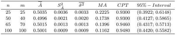
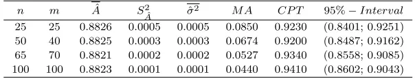
and the limiting availability isA=αβ/(αβ+λ). The simulation study considers 1000 repetitions for each simulation. We use the same notations and summary statistics used in the previous simulation. Table 3 and Table 4 present the results of the simulation.

Table 3: Simulation for a repairable system withα= 2.2,β= 2.1,λ=αβand limiting availabilityA= 0.5.

n m Aˆ S2

ˆ

A ˆσ

2 _{M A CP T 95%−Interval}

25 25 0.5035 0.0036 0.0033 0.2225 0.9300 (0.3922; 0.6148) 50 40 0.4996 0.0021 0.0020 0.1738 0.9300 (0.4127; 0.5865) 65 70 0.5015 0.0013 0.0013 0.1396 0.9460 (0.4317; 0.5713) 100 100 0.5001 0.0009 0.0009 0.1162 0.9480 (0.4420; 0.5582)

Table 4: Simulation for a repairable system with α = 5, β = 3, λ = 2 and limiting availabilityA= 0.8824.

n m Aˆ S2

ˆ

A ˆσ

2 _{M A CP T 95%−Interval}

25 25 0.8826 0.0005 0.0005 0.0850 0.9230 (0.8401; 0.9251) 50 40 0.8825 0.0003 0.0003 0.0674 0.9200 (0.8487; 0.9162) 65 70 0.8821 0.0002 0.0002 0.0527 0.9340 (0.8558; 0.9085) 100 100 0.8823 0.0001 0.0001 0.0440 0.9410 (0.8602; 0.9043)

3. Bayesian Estimation

In this section, we apply the Bayesian approach to the problem of estimation of the limiting availability. Specifically, we analyze the two repairable systems, which were described in the previous section. In this context, we must elicit a prior distribution for the limiting availability. This can be made by defining in a first stage prior distributions for the parameters of the observational model. The inference of the limiting availability will be based on its posterior distribution. We are considering two cases: informative and less informative prior distributions.

3.1. Elicitation of the Prior Distribution

Consider X the failure time with pdff(x|µ)andY the repairable time with pdff(y | λ), such that µX = µ, µY =λ, soA =µ/(µ+λ). Let µ ∼π(µ)and λ∼π(λ)be the prior densities forµandλ, respectively. Assuming independence, the joint prior for(µ, λ)is given byπ(µ, λ) =π(µ)×π(λ).

We are interested in determining the prior density of the limiting availability

A. So, consider the following change of variablesθ=A= _µ+µ_λ,ϕ=µ+λ. Then the joint distribution of the vector(θ, ϕ)is given by

π(θ, ϕ) = {

πµ(µ(θ, ϕ))πλ(λ(θ, ϕ))J((µ, λ),(θ, ϕ)), θ∈Θ,ϕ∈Φ,

0, θ̸∈Θ,ϕ̸∈Φ.

where µ(θ, ϕ) =θϕ and λ(θ, ϕ) =ϕ(1−θ). Also, Θis the parameter space of θ

andΦis the parameter space ofϕ.

The Jacobian of the transformation is given by

J((µ, λ),(θ, ϕ))=

∂µ ∂θ

∂µ ∂ϕ ∂λ ∂θ

∂λ ∂ϕ

=

ϕ θ

−ϕ 1−θ =ϕ.

Marginalizing, the prior density of θ=Ais

π(θ) = ∫

Φ

The following result is a direct extension of the characterization of the Beta distribution, through two independent Gamma random variables, with the same scale parameter. Although the proposition is a direct consequence of the work of Libby & Novick (1982), we prefer to include the demonstration in order to have a greater understanding in the reading of the article.

Proposition 1. If µ ∼ Gamma(a1, b1) and λ ∼ Gamma(a2, b2) then θ = A is Generalized Beta distributed with parameters (a1, a2, b1/b2), i.e., θ = A ∼

GB3(a1, a2, b1/b2).

Proof. We have

π(θ) = ∫ _∞

0

πµ(θϕ)πλ(ϕ(1−θ))ϕdϕ.

Then

π(θ) = ∫ _∞

0 ba1

1 Γ(a1)(θϕ)

a1−1_e−b1θϕb

(a2)

2

Γa2(ϕ(1−θ))

a2−1_e−b2ϕ(1−θ)_ϕdϕ

= b

a1

1 b a2

2 Γ(a1)Γ(a2)

θa1−1₍₁−_θ)a2−1

∫ _∞

0

ϕa1+a2−1_e−ϕ(b1θ+b2(1−θ))_dϕ

= b

a1

1 b a2

2 Γ(a1)Γ(a2)θ

a1−1₍₁−_θ)a2−1 Γ(a1+a2)

(b1θ+b2(1−θ))a1+a2

So,

π(θ)∝ θ

a1−1₍₁−_θ)a2−1

(

1−(1−b1

b2)θ

)a1+a2, 0< θ <1, (9)

this last expression corresponds to the kernel of a Generalized Beta density with parameters(a1, a2, b1/b2), see Chen & Novick (1996).

Note that, if b1 = b2 we obtain the usual beta distribution of parameters (a1, a2).

The calculus of the noninformative prior for the limiting availability is anal-ogous. In this part, we calculate the Jeffreys (1996) prior distribution for the limiting availability A. Considering the same scheme, the likelihood function of

(µ, λ)isL(µ, λ;x, y) =L(µ;x)L(λ;y).

Then the Fisher information matrix of(µ, λ)is given by

I(µ, λ) =     E (

−∂2logL(µ,λ;x,y) ∂µ2

) E

(

−∂2logL(µ,λ;x,y) ∂µ∂λ

)

E (

−∂2_{logL(µ,λ;x,y)}

∂µ∂λ )

E (

−∂2_{logL(µ,λ;x,y)}

∂λ2 )    ,

Analogously,

π(θ, ϕ) ∝ |I(µ(θ, ϕ), λ(θ, ϕ))|1/2J((µ, λ),(θ, ϕ)),

whereµ=µ(θ, ϕ) =θϕandλ=λ(θ, ϕ) =ϕ(1−θ). When it is possible, one must marginalizeπ(θ, ϕ)to obtain the noninformative prior for the limiting availability

θ=A.

3.2. Calculus of the Posterior Distribution

In this section, we calculate the posterior density function of the limiting avail-abilityA. Recall, the failure time X has a pdff(x| µ), µX =µ and the repair

time Y has a pdf f(x| λ), µY =λ. The limiting availability is A =µ/(µ+λ).

First, we reparametrize the likelihood function, considering θ = µ/(µ+λ) and

ϕ=µ+λ, which was used in the determination of the prior distribution in the previous section.

The likelihood function is L(µ, λ;x,y) = L(µ,x)×L(λ,y). Lettingµ = θϕ

andλ=ϕ(1−θ), the likelihood function becomes

L(θ, ϕ;x,y) =L(µ(θ, ϕ),x)×L(λ(θ, ϕ),y), whereθ∈Θ,ϕ∈Φ.

By the Bayes rule, the joint posterior density is

π(θ, ϕ|x,y) = ∫ L(θ, ϕ;x,y)π(θ, ϕ) Φ

∫

ΘL(θ, ϕ;x,y)π(θ, ϕ)dθdϕ ,

i.e.,

π(θ, ϕ|x,y)∝L(θ, ϕ;x,y)×π(θ, ϕ). (10) Marginalizing this last expression, we can obtain the posterior density ofθ=A,

π(θ|x,y) = ∫

Φ

π(θ, ϕ|x,y)dϕ. (11)

3.3. Bayesian estimation in an Exponential-Exponential

System

Consider a repairable system, where X = (X1, . . . , Xn) is a random sample

from the failure time with pdff(x|µ) =µe−µx_{, x >0, andY = (Y1, . . . , Ym)is}

a random sample from the repair time with pdff(y|λ) =λe−λy_{, y >0, m≤n.}

In this case the limiting availability is given byA=_(1/µ1₎₊₍₁/µ _/λ)= λ µ+λ.

The likelihood function is

L(µ, λ;x,y) =µnλmexp {

−µ n ∑

i=1 xi−λ

m ∑

j=1 yj

}

In the following proposition, we show that if one considers the usual prior Gamma for the parametersµ and λ, the Generalized Beta distribution is conju-gated. Furthermore, Bayes estimator and credible interval for the limiting avail-ability are computed.

Proposition 2. Supposeµ∼Gamma(a1, b1), λ∼Gamma(a2, b2), i.e., π(µ)∝ µa1−1_e−b1µ_{, µ > 0, π(λ)} ∝ _λa2−1_e−b2λ_{, λ > 0 and, µ and λ are independent.}

Then,

(i) The prior distribution ofA is a Beta Generalized distribution of parameters (a2, a1, b2/b1), i.e.,A∼ GB3(a2, a1, b2/b1).

(ii) A|x,y∼ GB3(a′₂, a′₁, b′₂/b′₁), wherea₁′ =a1+n,a′2=a2+m,b′1=b1+ ∑

xi andb′₂=b2+∑yj.

(iii) The Bayes estimator ofAand its risk are given by

b θB =

b′₁ b′₂

∞ ∑

j=0 (

1−b ′ 1 b′₂

)j_∏j

r=0

a′₂+r a′₁+a′₂+r,

b σ_B2 =

( b′₁ b′₂

)2 ∑∞ i=0 ∞ ∑ j=0 (

1−b ′ 1 b′₂

)i+j i+_∏j+1

k=0

a′₂+k a′₁+a′₂+k

−

(_∞ ∑

n=0 (

1−b ′ 1 b′₂

)n_∏n

r=0

a′2+r a′₁+a′₂+r

)2 

(iv) A credible interval of level1−αforAis given by (

a′₂b′₁

a′₁b′₂F1−α/2(2a′1,2a′2) +a′2b′1

; a

′ 2b′1

a′₁b′₂Fα/2(2a1′,2a′2) +a′2b′1 )

,

whereFα(ν, µ)is the α-percentile of the F distribution with(ν, µ)degrees of freedom.

Proof.

(i)It is a direct consequence of Proposition 1.

(ii)Consider the variable changes ofθ=A=λ/(λ+µ),ϕ=λ+µfor this case. Then marginalizing the joint posterior densityπ(θ, ϕ|x,y), we obtain

π(θ|x,y)∝ θ

a′₂−1_(1−θ)a′₁−1 (1−(1−b′2

b′₁)θ)

a′₁+a′₂, 0< θ <1,

which corresponds to the kernel of aGB3(a′₂, a₁′, b′₂/b′₁)distribution.

(iii) They are consequences of properties of Generalized Beta distribution. See Chen & Novick (1996).

(iv) Consider Pr(θ ≤ a | x,y) = Pr(θ ≥ b | x,y) = α₂, and use the fact that

a′₂b′₂ a′₁b′₁(

A

Remark. The non-informative case can be obtained by considering a1 → 0, b1→0, a2→0,andb2→0, in the prior densities.

3.4. Bayesian estimation in a Gamma-Exponential System

Consider a repairable system, where X = (X1, . . . , Xn) is a random sample

from the failure time with pdf f(x | α, τ) = 1 Γ(α)ταx

α−1_e−x/τ_{, x > 0, and}

Y = (Y1, . . . , Ym)is a random sample from the repair time with pdf f(y | λ) = 1

λe−

y/λ_{, y > 0, m ≤ n, where we suppose that α is known. In this case the}

limiting availability is given byA= _ατατ_+λ. The likelihood function is

L(τ, λ;α,x,y)

= τ

−nα λm_(Γ(α))nexp

{ (α−1)

n ∑

i=1

log(xi)−1 τ

n ∑

i=1 xi−

1 λ m ∑ j=1 yj } . (13)

In the following proposition, we show that if one considers the usual inverse-Gamma prior for the parameters τ and λ, the Generalized Beta distribution is conjugated. Furthermore, Bayes estimator and credible interval for the limiting availability are computed.

Proposition 3. Suppose τ ∼ inverse − Gamma(c1, d1), λ ∼ inverse − Gamma(c2, d2), i.e.,π(τ)∝µc1−1_e−d1µ_{, µ >0,π(λ)}∝_λc2−1_e−d2λ_{, λ >0 and,µ}

andλare independents. Then,

(i) The prior distribution ofA is a Generalized Beta distribution of parameters (c2, c1, d2/d1), i.e.,A∼ GB3(c2, c1, d2/d1).

(ii) A | x,y ∼ GB3(c₂′, c′₁, d′₂/d′₁), where c′₁ = c1+nα, c₂′ = c2 +m, d′₁ = α(d1+∑xi)andd′2=d2+

∑ yj.

(iii) The Bayes estimator ofAand its risk are given by

b θB =

d′₁ d′₂

∞ ∑

j=0 (

1−d ′ 1 d′₂

)j_∏j

r=0

c′₂+r c′₁+c′₂+r,

b σ_B2 =

( d′₁ d′₂

)2 ∑∞ i=0 ∞ ∑ j=0 (

1−d ′ 1 d′₂

)i+j i+_∏j+1

k=0

c′₂+k c′₁+c′₂+k

−

(_∞ ∑

n=0 (

1−d ′ 1 d′₂

)n_∏n

r=0

c′₂+r c′₁+c′₂+r

(iv) A credible interval of level1−αforAis given by (

c′₂d′₁

c′₁d′₂F1−α/2(2c′1,2c′2) +c′2d′1

; c

′ 2d′1

c′₁b′₂Fα/2(2c1′,2c′2) +c′2d′1 )

,

where Fα(ν, µ) is the α-percentile of F distribution with (ν, µ) degrees of freedom.

Proof. It is similar to the proof of Proposition 2.

3.5. Application and Simulation Study

Analogously to the classical case, we consider two systems with the same char-acteristics, where the times of the first system follow exponential distributions. In the other system, the failure time follows a Gamma distribution and the repair time, an exponential law. The computational implementation considers the follow-ing cases: conjugated informative priors, semi-informative priors, flat conjugated priors and non-informative priors.

3.5.1. Exponential-Exponential System

The parameters chosen for the simulations are presented in Table 5:

Table 5:Parameters for Simulations (Exp-Exp).

True parameters Prior parameters

Case µ λ A a1 b1 a2 b2

1.1 1.5 1.5 0.5000 0.5 1.0 0.5 1.0 2.1 1.2 5.5 0.8209 1.048 0.04 1.22 0.04 1.2 1.5 1.5 0.5000 1.0 1.5 1.0 1.5 2.2 1.2 5.5 0.8209 7.24 5.2 29.6 5.2 1.3 1.5 1.5 0.5000 61 30 61 30 2.3 1.2 5.5 0.8209 25.24 20.2 112.1 20.2

In cases 1.1 and 1.2, the parameters of the prior distributions are interesting to analyze. Cases 1.2 and 2.1 correspond to flat priors. Case 2.2 is a semi-informative prior. Cases 1.3 and 2.3 are informative priors, where the distribution is centred on the true parameters.

The distributions were simulated using R software version 3.4.1 (R Develop-ment Core Team 2007), each Bayesian estimator was obtained over 1000 real-izations and for different values of n and m. The estimators shown in Table 6 correspond to the average of the Bayesian estimators obtained on the 1000 rep-etitions. Also,n corresponds to the sampled units from the failure times andm

Table 6: Bayesian Estimation of the Limiting Availability (Exp-Exp).

Case n m µ λ A Ab.1 Ab.2 Ab.3 Abnon−inf

1 25 25 1.5 1.5 0.5000 0.4973 0.5008 0.4998 0.4975 2 25 25 1.2 5.5 0.8209 0.8154 0.8157 0.8172 0.8153 3 50 40 1.5 1.5 0.5000 0.4988 0.4976 0.5039 0.5038 4 50 40 1.2 5.5 0.8209 0.8179 0.8187 0.8182 0.8164 5 65 70 1.5 1.5 0.5000 0.5000 0.5005 0.4987 0.5010 6 65 70 1.2 5.5 0.8209 0.8191 0.8168 0.8187 0.8194 7 100 100 1.5 1.5 0.5000 0.5007 0.4998 0.4995 0.4979 8 100 100 1.2 5.5 0.8209 0.8197 0.8192 0.8201 0.8188

In Table 6, the subscript of the Bayesian estimator are in relation to the prior distribution used, for example if µ = 1.5 and λ = 1.5, and the estimate has subscript 2, then the parameters of the prior correspond to case 1.2 of Table 5.

We note that for the limiting availabilityA= 0.5, Bayesian estimators behave quite well. However, when limit availability increases, a fairly light underesti-mation is observed. The behavior of the estimate improves as the sample size increases.

Table 7: Mean Standard Deviation of the Bayesian Estimates (Exp-Exp) of the Limiting Availability.

Case n m µ λ A sd(Ab.1) sd(Ab.2) sd(Ab.3) sd(Abnon−inf)

1 25 25 1.5 1.5 0.5000 0.0682 0.0675 0.0379 0.0686 2 25 25 1.2 5.5 0.8209 0.0414 0.0332 0.0246 0.0423 3 50 40 1.5 1.5 0.5000 0.0519 0.0516 0.0342 0.0522 4 50 40 1.2 5.5 0.8209 0.0311 0.0264 0.0209 0.0317 5 65 70 1.5 1.5 0.5000 0.0425 0.0423 0.0311 0.0426 6 65 70 1.2 5.5 0.8209 0.0252 0.0231 0.0191 0.0254 7 100 100 1.5 1.5 0.5000 0.0350 0.0349 0.0278 0.0351 8 100 100 1.2 5.5 0.8209 0.0208 0.0193 0.0166 0.0210

Table 7 describes the mean of the standard deviations (sd) of the Bayesian estimates of the limiting availability. We observe that standard deviations decrease as prior distributions are more informative which is an expected behavior. Also, the sample sizes have some influence on the value of the standard deviations, but this influence is slight compared to the informative priors.

The 95%credibility regions are reported in Table 8, using the same notation as in Table 6. The length of the intervals tends to decrease as the sample size increases or when the priors distributions are more informative. When the limit availability is greater(A= 0.8209), the interval is more shifted to the left, this is due to the asymmetry of the posterior distribution of the limiting availability.

3.5.2. Gamma-Exponential System

Table 8: Mean Credibility Regions (CR) for Limiting Availability (Exp-Exp).

Case A CR.1 CR.2 CR.3 CRnon−inf

1 0.5000 (0.3643; 0.6307) (0.3689; 0.6325) (0.4256; 0.5740) (0.3637; 0.6316) 2 0.8209 (0.7247; 0.8861) (0.7452; 0.8749) (0.7663; 0.8625) (0.7223; 0.8874) 3 0.5000 (0.3968; 0.5998) (0.3961; 0.5981) (0.4368; 0.5707) (0.4011; 0.6052) 4 0.8209 (0.7509; 0.8726) (0.7630; 0.8663) (0.7751; 0.8570) (0.7481; 0.8721) 5 0.5000 (0.4170; 0.5832) (0.4178; 0.5834) (0.4379; 0.5596) (0.4177; 0.5844) 6 0.8209 (0.7659; 0.8647) (0.7688; 0.8591) (0.7796; 0.8543) (0.7658; 0.8653) 7 0.5000 (0.4322; 0.5693) (0.4314; 0.5682) (0.4452; 0.5539) (0.4292; 0.5666) 8 0.8209 (0.7764; 0.8577) (0.7792; 0.8548) (0.7861; 0.8511) (0.7752; 0.8572)

Table 9: Parameters for Simulations (Gamma-Exp).

True Parameters Prior Parameters

Case α τ λ A c1 d1 c2 d2

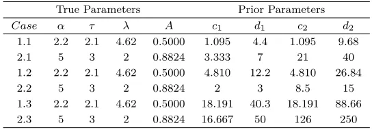
1.1 2.2 2.1 4.62 0.5000 1.095 4.4 1.095 9.68 2.1 5 3 2 0.8824 3.333 7 21 40 1.2 2.2 2.1 4.62 0.5000 4.810 12.2 4.810 26.84 2.2 5 3 2 0.8824 2 3 8.5 15 1.3 2.2 2.1 4.62 0.5000 18.191 40.3 18.191 88.66 2.3 5 3 2 0.8824 16.667 50 126 250

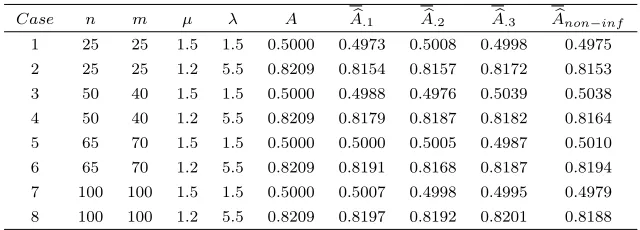
The parameters in Table 9 were chosen to study the behavior of the Bayesian estimation of limiting availability. The cases 1.1 and 2.1 correspond to a less informative prior, the cases 1.2 and 2.2 correspond to semi-informative priors and the rest to very informative priors. As in the previous case, the simulations are performed over 1000 repetitions for different values ofmandn, where the resulting estimator is the mean value of the 1000 Bayes estimators obtained. Table 10 summarizes the results of the estimates obtained.

Table 10: Bayesian Estimation of the Limiting Availability (Gamma-Exp).

Case n m α τ λ A Ab.1 Ab.2 Ab.3 Abnon−inf

1 25 25 2.2 2.1 4.62 0.5000 0.4970 0.4956 0.4981 0.5000 2 25 25 5 3 2 0.8824 0.8813 0.8815 0.8818 0.8786 3 50 40 2.2 2.1 4.62 0.5000 0.4976 0.4981 0.4987 0.4996 4 50 40 5 3 2 0.8824 0.8826 0.8826 0.8818 0.8807 5 65 70 2.2 2.1 4.62 0.5000 0.5000 0.4995 0.5011 0.5000 6 65 70 5 3 2 0.8824 0.8821 0.8817 0.8820 0.8817 7 100 100 2.2 2.1 4.62 0.5000 0.5009 0.5000 0.4997 0.5001 8 100 100 5 3 2 0.8824 0.8825 0.8824 0.8822 0.8817

We note that the estimates closely resemble the true value of the limiting availability. These estimates are more accurate as the sample size increases. The standard deviations are presented in Table 11.

Table 11: Standard Deviation (sd) of Bayesian Estimates of Limiting Availability (Gamma-Exp).

Case n m α τ λ A sd.1 sd.2 sd.3 sdnon−inf

1 25 25 2.2 2.1 4.62 0.5000 0.0582 0.0552 0.0476 0.0592 2 25 25 5 3 2 0.8824 0.0181 0.0206 0.0122 0.0238 3 50 40 2.2 2.1 4.62 0.5000 0.0451 0.0436 0.0392 0.0456 4 50 40 5 3 2 0.8824 0.0149 0.0164 0.0103 0.0181 5 65 70 2.2 2.1 4.62 0.5000 0.0360 0.0352 0.0329 0.0362 6 65 70 5 3 2 0.8824 0.0124 0.0132 0.0093 0.0138 7 100 100 2.2 2.1 4.62 0.5000 0.0299 0.0294 0.0280 0.0300 8 100 100 5 3 2 0.8824 0.0105 0.0110 0.0083 0.0115

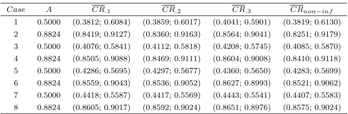
Table 12 reports the95%credibility regions, using the same notation as in Table 11. The length of the intervals tends to decrease as the sample sizes increase or when the priors are more informative.

Table 12: Credibility Region (CR) of Limiting Availability (Gamma-Exp).

Case A CR.1 CR.2 CR.3 CRnon−inf

1 0.5000 (0.3812; 0.6084) (0.3859; 0.6017) (0.4041; 0.5901) (0.3819; 0.6130) 2 0.8824 (0.8419; 0.9127) (0.8360; 0.9163) (0.8564; 0.9041) (0.8251; 0.9179) 3 0.5000 (0.4076; 0.5841) (0.4112; 0.5818) (0.4208; 0.5745) (0.4085; 0.5870) 4 0.8824 (0.8505; 0.9088) (0.8469; 0.9111) (0.8604; 0.9008) (0.8410; 0.9118) 5 0.5000 (0.4286; 0.5695) (0.4297; 0.5677) (0.4360; 0.5650) (0.4283; 0.5699) 6 0.8824 (0.8559; 0.9043) (0.8536; 0.9052) (0.8627; 0.8993) (0.8521; 0.9062) 7 0.5000 (0.4418; 0.5587) (0.4417; 0.5569) (0.4443; 0.5541) (0.4407; 0.5583) 8 0.8824 (0.8605; 0.9017) (0.8592; 0.9024) (0.8651; 0.8976) (0.8575; 0.9024)

4. Bayes estimation in a Case Study

In the packing process in a certain glass bottles Chilean factory, a machine (handled by a trained worker) called palletizer is used.

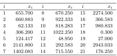
Table 13: Failure times (in hours).

i xi i xi i xi

1 655.700 8 670.250 15 2274.500 2 660.883 9 922.333 16 366.583 3 62.133 10 818.283 17 980.833 4 306.200 11 1022.250 18 0.300 5 124.417 12 48.950 19 27.000 6 2141.800 13 292.583 20 2943.033 7 1402.083 14 715.550 21 176.250

Table 14: Descriptive statistics for failure times. Statistic V alue

Sample size 21 Minimum 0.3000 Maximum 2943.0333

Median 660.7000 Mean 791.0437 Variance 648486.8 Standard deviation 805.2868

Table 15: Repair times (in hours).

j yj j yj j yj

1 0.4167 8 0.0833 15 0.5000 2 0.2000 9 0.3000 16 0.5000 3 0.0500 10 1.3333 17 0.0333 4 0.1667 11 0.6333 18 0.0833 5 0.0333 12 0.5833 19 0.1333 6 1.4167 13 0.1167 20 1.5000 7 0.2500 14 0.1667 21 0.1667

Table 16: Descriptive statistics for repair times.

Statistic V alue

Sample size 21 Minimum 0.0333 Maximum 1.5000 Median 0.2000 Mean 0.4127 Variance 0.2099 Standard deviation 0.4582

The Kolmogorov-Smirnov test is applied both for the failure times and for the repair times considering the exponential distribution as the null hypothesis. This was done using the SAS software Version[9.4] (SAS 2017), obtaining a p-value greater than 0.5. So, the density functions of the failure time and the repair time are considered asf(x|λ) =λe−λx_{, x >0and f(x|µ) =µe}−µy_{, y >0. Since we}

Failure times

Hours

Density

0 500 1000 1500 2000 2500 3000

0.0000

0.0002

0.0004

0.0006

0.0008

0.0010

0.0012

0 500 1000 1500 2000 2500 3000

0.0000

0.0002

0.0004

0.0006

0.0008

0.0010

0.0012

Repair times

Hours

Density

0.0 0.5 1.0 1.5

0.0

0.5

1.0

1.5

2.0

2.5

0.0 0.5 1.0 1.5

0.0

0.5

1.0

1.5

2.0

2.5

Figure 1: Histogram for failures (left) and repair times (right) with exponential densities

for the palletizer data.

π(θ|x, y)∝ θ

21₋1_(1−θ)21₋1

(16611.9 +θ(8.667−16611.9))42,0< θ <1. (14)

Note that, n = m = 21, ∑xi = 16611.9 and ∑

yj = 8.667. A graph of

this density is presented in Figure 2, which accounts for its asymmetry, with high probabilities at the upper end. Consequently, this is reflected in the estimates that are described in Table 17 and in the95%credibility region which is given by

CR= (0.99904,099972). The results obtained show that the palletizer is working in optimal conditions. However, periodically its use must be monitored.

0.9985 0.9990 0.9995 1.0000

0

500

1000

1500

2000

2500

Limiting Availability

P

oster

ior density Limiting A

v

ailability

Table 17: Bayes estimation of the limiting availability for the palletizer data.

Estimates V alue b

A 0.9994534

d

V ar(Ab) 2.697561×10−13 d

s.d.(Ab) 5.193805×10−7

5. Conclusions

In the present work, the problem of estimating the limiting availability in a single-component system is addressed under a Bayesian methodology. Also, the maximum likelihood estimate is revisited.

When implementing the maximum likelihood estimate, the behavior of the estimators is consistent as the sample size is increased. Clearly, the convergence of the estimator is affected by the dispersion of each variable.

In the Bayesian case, the simulations were performed in a rather general way. Exponential and Gamma distributions were considered for the failure time and the repair time. The use of exponential and Gamma distributions for failure and repair times has been motivated, taking into account the referential frame they have in reliability. In addition, in our case, it is possible to perform a conjugate analysis, taking as a priori the generalized Beta distribution. Furthermore, differ-ent types of prior distributions for the hyperparameters were considered. In the first instance, priors providing little information and then others more informative. Estimates of limiting availability greater than 0.5 are slightly underestimated in both the classical and Bayesian cases when the failure time and the repair time are exponential. However this does not occur, when the fault time is distributed Gamma and the repair time, exponential.

A relevant point of this work is to have developed a general Bayesian method-ology, since this is not limited to the particular distributions considered.

The Bayesian method is applied in the estimation of the limiting availability of a palleitzer of a glass bottles factory, without having prior information. The results reflect the good performance of the machine.

Extensions of this approach include the use of other loss functions, which could help to control underestimation (respectively overestimation). In fact, the Bayesian methodology developed and applied in this paper can be adapted to a co-herent system ofkindependently functioning components. Also, other parametric models used in reliability system can be considered.

One interesting approach is to set up the reliability model treated in this paper in a Bayesian semiparametric framework. This is a topic, for future research.

Acknowledgements

of Chile. We are immensely grateful to the referees for their comments on an earlier version of the manuscript.

[

Received: June 2017 — Accepted: November 2018]

References

Abraham, B. & Balakrishna, N. (2000), ‘Estimation of limiting availability for a stationary bivariate process’, Journal of Applied Probability37(3), 696–704. Ananda, M. (1999), ‘Estimation and testing of availability of a parallel system

with exponential failure and repair times’, Journal of Statistical Planning and Inference 77(2), 237–246.

Barlow, R. & Proschan, F. (1996),Mathematical Theory of Reliability, classics in applied probability edn, SIAM, New York.

Baxter, L. & Li, L. (1994), ‘Non-parametric confidence intervals for the re-newal function and the point availability’,Scandinavian Journal of Statistics 21, 277–287.

Baxter, L. & Li, L. (1996), ‘Nonparametric estimation of the limiting availability’,

Lifetime Data Analysis2, 391–402.

Chen, J. & Novick, M. (1996), ‘Bayesian analysis for binomial models with gener-alized Beta prior distributions’,Journal of Educational Statistics9, 163–175. Huang, K. & Mi, J. (2013), ‘Properties and computation of interval availability of

system’,Statistics and Probability Letters83, 1388–1396.

Jeffreys, H. (1996),Theory of Probability, 3 edn, Oxford University Press, Oxford.

Kaplan, E. & Meier, P. (1958), ‘Nonparametric estimation from incomplete obser-vations’, Journal of the American Statistical Association53, 457–481. Libby, D. & Novick, M. (1982), ‘Multivariate generalized beta-distributions with

applications to utility assessment’, Journal of Educational Statistics7, 271– 294.

Lu, M. & Mi, J. (2011), ‘ Statistical inference about availability of system with gamma lifetime and repair time’,Statistics and Probability Letters18, 1–24. Marsan, M., Balbo, G., Conte, G., Donatelli, S. & Franceschinis, G. (1995), Mod-elling with Generalised Stochastic Petri Net, Dipartimento d´Informatica, Universit degli Studi di Torino, Torino, Italy.

Mi, J. (1991), ‘Interval estimation of availability of a series system’,IEEE Trans-actions on ReliabilityR-40, 541–546.

Mi, J. (2006), ‘Limiting availability of system with non-identical lifetime distribu-tions and non-identical repair time distribudistribu-tions’, Statistics and Probability Letters76, 729–736.

Mishra, A. & Jain, M. (2013), ‘Availability ofk-out-of-n: F secondary subsystem with general repair time distribution’, International Journal of Engineering Transactions A: Basics26, 743–752.

R Development Core Team (2007),R: A Language and Environment for Statistical Computing, R Foundation for Statistical Computing, Vienna, Austria. ISBN 3-900051-07-0.

*http://www.R-project.org

Ross, S. (1996),Stochastic Processes, 2 edn, Wiley, New York.

Sarkar, J. & Chandhuri, G. (1999), ‘Availability of a system with gamma life and exponential repair time under a perfect repair policy’, Statistics and Probability Letters 43, 189–196.

SAS (2017), SAS software, Version [9.4] of the SAS System for [Microsoft Win-dows Workstation for x64], SAS Institute Inc., North Caroline, U.S.A. Copy-right c⃝2017.

Sethuraman, J. & Hollander, M. (2009), ‘Nonparametric Bayes estimation in repair models’,Journal of Statistical Planning and Inference139, 1722–1733. Sobolewski, R. (2016), ‘Implication of availability of an electrical system of a wind

farm for the farm’s output power estimation’,Advances in Intelligent Systems and Computing470, 1722–1733.

Thompson, W. & Palicio, P. (1975), ‘Bayesian confidence limits for the availability of systems’,IEEE Transactions on ReliabilityR-24, 118–120.

Vásquez, C. (2006), Estimation of the limiting availability in a reliability system, Statistical Engineer Thesis, Universidad de Santiago de Chile, Facultad de Ciencia. Departamento de Matemárica y Ciencia de la Computación.

MASSEY RESEARCH ONLINE

http://mro.massey.ac.nz/

Massey Documents by Type Journal Articles

Bayesian estimation of the limiting

availability in a repairable one-unit system

Vasquez, C

2019-01-01

http://hdl.handle.net/10179/14380