Rans modelling of intermittent turbulent flows using adaptive mesh refinement methods

This is a repository copy of

Rans modelling of intermittent turbulent flows using adaptive

mesh refinement methods

.

White Rose Research Online URL for this paper:

http://eprints.whiterose.ac.uk/83556/

Version: Accepted Version

Article:

Olivieri, DA, Fairweather, M and Falle, SAEG (2010) Rans modelling of intermittent

turbulent flows using adaptive mesh refinement methods. Journal of Turbulence, 11 (29). 1

- 18. ISSN 1468-5248

https://doi.org/10.1080/14685248.2010.499129

[email protected]

https://eprints.whiterose.ac.uk/

Reuse

Unless indicated otherwise, fulltext items are protected by copyright with all rights reserved. The copyright

exception in section 29 of the Copyright, Designs and Patents Act 1988 allows the making of a single copy

solely for the purpose of non-commercial research or private study within the limits of fair dealing. The

publisher or other rights-holder may allow further reproduction and re-use of this version - refer to the White

Rose Research Online record for this item. Where records identify the publisher as the copyright holder,

users can verify any specific terms of use on the publisher’s website.

Takedown

If you consider content in White Rose Research Online to be in breach of UK law, please notify us by

Rans Modelling of Intermittent Turbulent Flows Using Adaptive

Mesh Refinement Methods

D.A. Olivieria_{, M. Fairweather}a_{and S.A.E.G. Falle}b

a_{School of Process, Environmental and Materials Engineering, The University of Leeds,}

Leeds LS2 9JT, UK; School of Mathematics, The University of Leeds, Leeds LS2 9JT, UK

This paper investigates the modelling of intermittency in turbulent jet flows using the Reynolds-averaged Navier-Stokes flow field solutions, coupled to the solutions of the transported probability density function (PDF) equation for scalar variables, obtained using a finite-volume method combined with an adaptive mesh refinement algorithm applied in both physical and compositional space. The effects of intermittency,, on the turbulent flow field are accommodated using a k-- turbulence model as well as being applied in the mixing model embodied within the transported PDF equation. Different mixing models are also considered for use with the latter transport equation, including the linear mean square estimation and the Curl and Langevin approaches. Results are compared with the available experimental data on a jet flow with good agreement obtained.

Keywords: Reynolds-averaged Navier-Stokes; transported PDF; finite-volume; adaptive mesh refinement; intermittency

1. Introduction

Turbulent shear flows with free boundaries display an intermittent character, where the flow rapidly alternates between rotational and irrotational states. Intermittency can be thought of as an indicator function that has a value of unity when the flow is turbulent and zero when it is non-turbulent, i.e. it represents the fraction of time during which a point is inside the turbulent fluid.

The intermittent behaviour of flows is influential in many processes of practical relevance, including mixing, combustion, pollutant emissions and aeroacoustics. For example, the safe and efficient operation of many combustion devices is critically dependent on ignition occurring in regions of the flammable flow, which contain significant intermittency. Enhancing the performance of these devices, and improving their safety, in particular, relies on a better understanding of both the intermittent flow and the ignition process.

The majority of turbulence models currently in use were derived for fully developed flows, and hence cannot be expected to perform accurately in free shear flows where the outer regions are contaminated with irrotational flow. Intensive research efforts have been devoted to developing more general engineering models of turbulence in recent years, although their predictability remains largely dependent on flow configuration. The development of more accurate and broadly applicable models of turbulence can, however, be accomplished by accommodating intermittency effects within these models. A good example of this is seen in the round jet/plane jet anomaly [1], where the inclusion [2] of intermittency effects within a conventional k- turbulence model was demonstrated to resolve this anomaly. In these, and many other free and wall-bounded flows [2], the inclusion of intermittency effects, therefore, helps to generalise existing turbulence models, and provide more accurate predictions of the velocity and scalar fields of interest in the applications noted above. Such intermittency-based models are also required in order to predict boundary layer transition.

single scalar within a turbulent jet flow. Olivieri et al [3] have previously demonstrated the application of an AMR finite-volume technique in physical and compositional space, with the latter permitting solution of the transported PDF equation. This contrasts with more conventional approaches, which are based on the use of finite-volume methods in physical space, and Monte Carlo methods in compositional space for solution of the PDF equation. The latter work [3] also demonstrated that, for small numbers of scalar variables, AMR provides improved accuracy, run times and ease of use over alternative Monte Carlo approaches. The effects of intermittency on the turbulent flow field have been accommodated in a conventional Reynolds-averaged Navier-Stokes (RANS) approach using thek--model of Cho and Chung [2], with the influence of on the PDF included via the mixing model embodied within its transport equation. This contrasts to the earlier approach of Kollmann and co-workers [4-7], which used a finite-difference approach to solving the PDF transport equation coupled to a closure scheme based on conditional zone-averaged moments, rather than the Reynolds averaged moments used in the present work.

AMR is now a well-established technique. The earliest applications were to two-dimensional shock problems [8, 9], with later extensions including three-two-dimensional problems [10] and implementation on parallel computers [11]. The advantage of AMR is that it can use error estimates to adaptively increase numerical grid resolution to meet accuracy requirements in specific parts of physical space, and conversely reduce resolution in regions of the flow where few changes are taking place. The approach offers particular advantages for transient problems with travelling discontinuities, such as shocks. Previous work by the authors [3] has also extended this technique to compo-sitional as well as physical space. In some classes of problems, CPU and memory requirements can be reduced over those for a uniform grid by as much as a factor of one hundred [12].

2. Mathematical modelling 2.1Fluid flow equations

N

Here u˜ andv˜ are the mean velocities in the z andr directions, and _k, _ and _ are the Prandtl numbers for k,  and , and the superscript tilde denotes density-weighted averaging. Due to the thin shear layer approximation, only the u˜-component of the mo- mentum equation is employed. The turbulence energy dissipation rate equation involves a modification to its source term, this being the term shown in square brackets. The Galilean invarianceused in modifying this source represents the amount of intermittency entrained by the interaction between the mean velocity gradient and the intermittency, per unit volume of the fluid field. When the flow intermittency is small, small-scale eddies in the flow are relatively inactive and the turbulence kinetic energy is dissipated slowly. If intermittency is large, then small eddies become embedded in the large straining eddies in the interactive shear layer between the turbulent and irrotational zones. The parameter, therefore, indicates how much of a source or sink of dissipation is occurring due to the entrainment of more-irrotational fluid at the particular point under consideration. The turbulent viscosity µ and the Galilean invarianceare given as follows:

where U is the total flow velocity vector. Note that for the thin shear layer approximation |U|

u˜. _{The final expression provides a transport equation for itself. The} first term on the

right-hand side of this equation describes the bulk convective spatial transport due to turbulent flow, while the other terms on the right-hand side contribute to the source term, which describes the mean rate of entrainment of non-turbulent fluid into the turbulent zone. The source term of this equation represents the main part of the Cho and Chung model [2]. Pressure is assumed to be constant, which avoids the need for a Poisson equation solver, and as will be demonstrated in Section 4, this is a good approximation for the considered jet flow. It is also unnecessary to solve the continuity equation because the density can be calculated from the average of the mass fraction< >of each species :

where is the density of a fluid comprising only species .

2.2. Scalar PDF equation

As this work concerns non-reacting turbulent flows, the PDF equation employed only involves the use of a passive scalar, which is the mixture ratio . This means thatN = 1 and = for the compositional space of a single species, and that in Equation (3) the realisation of the scalar from the compositional space is< >. Hence, for a pure fuel flow,< >= 1 and for a pure oxidant,< >= 0. Equation 3 can therefore be rewritten as

Here, _pis the Prandtl number for the turbulent diffusion of P. Equation (5) is based on the full scalar PDF transport equation for chemically reactive flows [14].

2.3. Molecular mixing

The molecular mixing term in Equation (5) has a number of models available to represent its effect, with the simplest being the linear mean square estimation (LMSE) method [14]. If the standard model is modified to take into account the effect of, the expression for the LMSE mixing becomes

HereC_D,andkare the ratio of the scalar to mechanical turbulent time scales, the viscous dissipation rate of turbulence kinetic energy and the turbulence kinetic energy per unit mass [14]. The justification for implementing  in Equation (6) in this way is due to the fact that the magnitude of has a direct bearing on the molecular mixing only and not on the other terms given in Equation (5). Similar reasoning was used previously by Kollmann and Janicka [7].

There are other possibilities for this term: the coalescence/dispersion or Curl model [15, 16] and the Langevin model [14]. However, the Curl model is computationally expensive because it involves an integro-differential equation. In Olivieri et al [3], application of the basic version of the Curl model was considered. In the present work, a modified Curl model [7, 17] that preservesP is considered as a source term, and not an advective term, for the scalar :

Again,  is incorporated in a similar way in the mixing model as it was with the LMSE model. Later on in Section 4 the two models are compared with experimental results as a way of assessing the accuracy and effectiveness of each approach.

Higher order molecular mixing models, such as the Langevin model [14], unfortunately failed when applied to bounded scalars. Other approaches involving binomial models, such as that of Valino and Dopazo [18], have been suggested as a way of avoiding this shortcoming. However, although the model has been shown to work well for PDFs of single scalars with fixed bounds, it is not squarely applied with multiple scalars. Therefore, only the LMSE and the modified Curl models [17, 19] are applied to predict intermittency in the flow considered below, given the authors’s ultimate interest lies in extending the work described herein to ignition processes and combusting flows.

2.4. von mises coordinates

It is a standard practice [13] to write Equations (2) in terms of the von Mises coordinates, ( , z), which automatically satisfies mass conservation:

where

Equations (2) then become

The turbulent viscosity µ and the Galilean invariance of the scalarare also to be redefined as follows:

These equations are simply evolution equations, withzplaying the role of the time-like coordinate. If we apply von Mises coordinates to the PDF, Equation (5) becomes

The last term in Equation (11) represents molecular mixing as is the case with Equation (5).

3. Numerical method 3.1. Finite-volume scheme

Equation (10) contains only diffusive fluxes, while Equation (11) contains both advective (the LMSE molecular mixing term in the PDF equation) and diffusive fluxes. For the modified Curl mixing model case, Equation (11) has only diffusive fluxes, with a source term for the molecular mixing term itself. In order to construct a numerical scheme, physical space is discretised with mesh spacing , and composition space with mesh spacing . For the fluid quantities, mean quantities in a cell atz=z_n are defined as follows:

whereqis one of (u˜, k,,). For the PDF, a mean value atz=z_n is defined by averaging over both physical and composition space:

i

wherefil, firare approximations to the fluxes at the left/right edges of theith cell andsi is an

approximation to the source term. Also,

An approximation that is of first order inz is obtained if values atznare used to compute

the fluxes and the source terms. The source terms can be calculated from the mean values in the cell. In order to compute the fluxes, approximations to the flow variables andrat the cell edges are required. The flow variables can be computed from simple averages,

The radius at the cell edges is obtained using the trapezoidal rule to integrate Equation (8)

This gives a simple recurrence relation for theril. The flux for quantityqis then given by

whereµr is calculated from the flow variables at the cell edge. As this is a central difference approximation to diffusive terms, the resulting scheme is of second order in . The procedure forP is similar, and involves no advection because the flow is non-reacting, apart from the minor advective effect due to molecular mixing. With the LMSE approximation, the effective advective velocity in composition space is

The PDF is then updated via

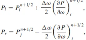
where (P)_p is the increment due to the diffusive term in physical space. A first-order upwind approximation is obtained by setting the flux at a cell face to

wherePl n

andPr n

are the values in the cells on the left- and right-hand side of the cell face. Here ˙ is evaluated at the centre of the cell face. For the molecular mixing case involving the Curl model, Equation (19) is rewritten such that

where s´_i is an approximate source term representing the modified Curl molecular mixing model, evaluated at the compositional cell centre = _iwith the expression given in Equation (7) using numerical integration. The numerical scheme presented so far is of second order inr, but of first order inz and . In order to make it of second order in all variables, we first use the first-order scheme to compute an intermediate solution, fin+1/2, at the half-stepzn+1/2 = (zn +zn+1)/2. These values are then used to compute the fluxes and source terms for the flow variables, which are subsequently used to update them through a complete timestep i.e.

The same is done for the flow terms in the PDF equation, but in order to obtain second-order accuracy in , a better approximation to the advective fluxes in composition space is required:

wherea(a, b) is a non-linear averaging function and the subscriptslandr denote values in the neighbouring cells on the left- and right-hand side. It is essential to use a non-linear averaging function here because Godunov’s theorem [20] tells us that a scheme that is of second order everywhere will generate oscillations where the solution changes rapidly. This applies in this case if the PDF approaches a delta-function, but if it is smooth, then one can use a simple average.

The gradients given by Equation (23) are then used to obtain a better approximation tof at a cell face. For example, for a cell face the values offl andfr to be used in Equation (20)

are given by

whereiandj are the cells on the left- and right-hand side of the face. The final solution at z =z_n+1 is then obtained from Equation (19) using these values of P_land P_r. This is essentially the same scheme as that described in [21] for compressible flow. Although it is not as accurate as some schemes for linear advection, it is robust and simple to implement.

3.2. Adaptive mesh refinement

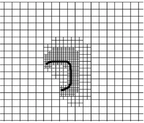
Unlike most AMR approaches, e.g. [8-12], in the present work, refinement is on a cell-by-cell basis instead of being organised into patches. This provides a more efficient grid at some increased cost of integration. Figure 1 shows how this works in two dimensions for a thin region, such as a shear layer that requires high resolution. A hierarchy of uniform grids G0··· GL is used so that if the mesh spacing onG0is ( ,  ), then it is ( /2n, /2n) on

Gn. Grids G0andG1cover the whole computational domain, but the finer grids need only

exist in regions that require high resolution. The grid hierarchy is used to generate an estimate of the relative error by comparing solutions on grids with different mesh spacings, and the grid is then refined if this error exceeds a toleranceEr and de-refines if it is less

thanEd. Refinement also occurs inzso that if the step onG0 isz, then it isz/2nonGn.

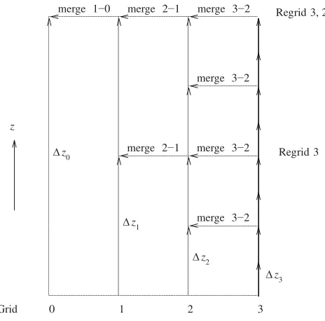
The integration algorithm is recursive and is described by a pseudo-code for the integration of grid Gnover its z step. From the pseudo-code given below, the procedure

integrate(0) performs integration on all grids through one G0 grid z-step, z up to a

maximum of Lmax possible levels of refinement. This process is shown schematically in

Figure 1. Grid refinement at a region requiring high resolution (represented by thick black curve).

In themerge(n)operation, the solution in the cells onG_nthat are refined is replaced by the volume average of the solutions in theG_n+1cells that it contains. This ensures that the solutions on all grids are consistent.

procedure integrate(n){ Integrate G_n

step(n) Advance G_nby one z-stepz/2n−1 if (n <(L_max)){ Finer grids exist

while (z_n < z_n−1){

integrate(n+1) Integrate G_n+1 to G_nz

z_n =z_n+z/2n Increment G_nz by

z

_/2

} end of while loop

regrid(n) Compare solutions on G_nand G_n−1 decide G_n+1 refinement merge(n) Project G_n+1solution onto G_n

} end of if block

return

} end of procedure integrate(n)

∆z 0

merge 2−1

merge 3−2

merge 3−2

∆z 1

merge 3−2

∆z 2

merge 1−0 merge 2−1 merge 3−2 _{Regrid 3, 2}

z

Regrid 3

∆z 3

Grid 0 1 2 3

Figure 2. Integration of a four level grid.

In order to allow different levels of refinement in physical and compositional space, a complete composition space hierarchy is associated with each physical cell on every grid level. The number of levels of refinement of the composition space in a particular physical cell is then determined by the accuracy requirements for that particular cell. So, for example, the maximum number of grid levels will be used in composition space ifP is close to a delta-function, whereas a smaller number of levels will be used if it is smooth.

Table 1. Parameters used in the computations.

Levels of adaptation 4 (physical space), 4 (compositional space) No. of coarse cells 30 (physical space), 25 (compositional space)

Turbulence model constants Cµ = 0.09,Cµ = 0.1,C1 = 1.44,C2 = 1.92

C₄ = 0.1,C₁ = 1.6,C₂ = 0.15,C₃ = 0.16 CD = 4, k = 1,  = 1.3,  = 1, p = 1

Nozzle diameter (d) 0.00526 m

Jet density 1.8638 kg m−3

Co-flow density 1.1964 kg m−3

4. Results and discussion

In order to verify and validate the modelling strategy described above, a series of qualitative and quantitative tests have been made involving the mixing of a single passive scalar in a non-reactive jet. All calculations are based on the experimental work of Schefer and Dibble [22], who studied a non-reacting propane jet in a co-flowing air stream. The parameters of the problem are given in Table 1. The first set of tests makes a qualitative appraisal of the effect of on the transported PDFP at a point 20 jet diameters downstream, while the second set of tests investigates how well different molecular mixing models perform compared with the experimental data [22].

4.1. Effect of intermittency on the transported PDF

The distribution of the PDFP against the passive scalar is given in Figure 3 atz/d =20 and for a number of radial locations. Each distribution of P was derived from the compositional space associated with a particular physical space region, and represents the different evolutionary changes inP at a particular downstream location due to the influence of the momentum change in the physical flow field and local molecular mixing effects. All results shown in this figure were derived using the LMSE mixing model.

On the axis of symmetry atr/d = 0 (Figure 3(a)), the distribution of P is approximately Gaussian because the flow is fully turbulent. With increases in radial distance, the PDF evolves until at r/d = 1.68 and r/d = 2.16 the distribution is clearly bi-modal due to the intermittent nature of the flow, as described previously. These PDF distributions are comparable with those predicted by Kollmann and Janicka [7], with the latter authors and the current approach including the influence of  in the scalar dissipation terms, and not in the turbulent transport of the PDF terms. The present approach differs from that of Kollmann and Janicka’s [7] in terms of the method used to determine , as has been indicated in Section 2, where in this work it is obtained through the solution of the conservation equations, rather than through the zone-averaged stress equation approach. In Kollmann and Janicka [7], and Pope [23], the PDF distributions are therefore the sum of continuous and singular contributions. By using the approach of Cho and Chung [2] to calculate, as employed herein, the sub-division of the PDF is unnecessary. This avoids the need for complex functions that the dissipation terms of [7] and [23] involve. In the case of the LMSE molecular mixing model, it also provides a very simple and computationally inexpensive method of incorporating the effects of intermittency. With the modified Curl mixing model, results for which are not shown here but later in Figures 6 to 9, the complex integro-differential function given in Equation (7) offers no greater benefit in terms of accuracy, and in fact is computationally prohibitive, particularly for multi-scalar modelling.

Figure 3. Effect of the intermittency on predictions of the scalar PDF atz/d= 20 and at different radial positions: (a) effects included; (b) no effects included (solid liner/d = 0, dashed liner/d= 0.834, dotted liner/d = 1.276, dot-dashed liner/d= 1.68, dot-dot-dashed liner/d=2.16); (c) and (d) show, at two scales, effect of varyingCD on PDF atz/d= 20 andr/d= 1.68 (dot-dashed lineCD = 0, dotted

Figure 3(b) shows results for the PDF derived without the effects of included in the expression for (∂P/∂t)mm. As a result, the distributions of P from each compositional

space associated with the physical domain at different radial positions across the jet do not take on a bi-modal shape at any location and, as will be seen later, fail to predict experimental [22] observations. Also, in the results of Figure 3(a), not only is the influence of the inclusion of intermittency clearly observable on the PDF but, as will be seen later, its influence in modifying the PDF is also subsequently fed back to the flow equation solutions as the coupled physical/compositional space method proceeds with the nextz step.

In Figure 3(c), and at an expanded scale in Figure 3(d), the impact of CD is

investigated for a particular PDF distribution from Figure 3(a), i.e. atr/d= 1.68. A value of CD= 4.0 is used in all the results discussed below because such a value was found to give

the most accurate predictions in comparison with experimental data. As this value is reduced, the variance naturally increases until atCD= 0 there are no longer any molecular

mixing effects involved in the calculations. At this point, the second term from Equation (11) is responsible for the two spikes at either end of the axis for the passive scalar as shown in Figure 3(d). Pope’s [14] considerations of scalar dissipation indicate that it is not possible forCDto be universally constant, with the latter work considering variations of this

constant between 0.6 and 3.1. From what has been discussed so far, the value of CD

clearly has a significant bearing on the accuracy with which the scalar second moments are determined.

Figure 6. Comparison of the measured and the predicted mixture fraction and rms of mixture fraction fluctuations along centre-line of jet (symbols – experimental data [22], solid line – predicted using LMSE with included, dotted line – predicted using LMSE without included, dashed line – predicted using the Curl mixing model with included).

Figure 8. Comparison of the measured and the predicted distributions of the scalar PDF at different locations along jet centre-line: (a)z/d= 5.2; (b)z/d= 7.1; (c)z/d= 10.8; (d)z/d= 15.0; (e)z/d= 30.0 and (f)z/d= 64.0 (symbols – experimental data [22], solid line – predicted using LMSE with included, dotted line – predicted using LMSE withoutincluded, dashed line – predicted using the Curl mixing model with included ).

4.2. Effect of intermittency and molecular mixing model on jet flow predictions

Figures 4 to 7 compare predictions of the model described with mean and turbulent flow quantities measured by Schefer and Dibble [22], and Figures 8 and 9 comparing the PDF distributions along the jet centre-line and also radially within the jet. Results are shown for predictions based on the LMSE molecular mixing model, with the effects of intermittency included and excluded to allow an assessment of its impact on the mixing field, and for the modified Curl mixing model with intermittency effects included. The predictions given for the velocity field and for intermittency, in Figures 4, 5 and 7, are applicable to all the mixing models considered, and are based on solutions of the fullk--turbulence model [2].

Figures 4 and 5 demonstrate reasonable agreement between predictions and observations for the velocity field, and the approximation of constant pressure used in this work appears justifiable in view of these results. Predictions of the normal and shear stresses shown in these figures, in particular, could be improved further with the application of a second moment turbulence closure, coupled to a transport model for the intermittency, as has been previously demonstrated by Alvani and Fairweather [24]. The current results are, however, comparable to those obtained in [25] by the latter authors when using ak--turbulence modelling approach. The various mixing models considered had little effect on the results given in these figures.

Figures 6 and 7 show results for the first and the second moments of the passive scalar at various locations in the flow field. In both the figures the scalar means< >, shown as

˜, predicted that using the various mixing models are comparable throughout the flow field, apart from the radial profile at z / d= 50 in Figure 7, where predictions obtained using the LMSE model with intermittency effects included are clearly superior. Overall, however, the calculated ˜ agree reasonably well with the experimental data. This is not the case for the scalar second moments, , however, where predictions obtained using the LMSE and the Curl models clearly differ. The results presented in these figures indicate that the LMSE model with effects included provides the most accurate predictions over the majority of the flow field. As well as being less accurate, the modified Curl molecular mixing model also proved to be much more computationally expensive because of its use of an integro-differential equation. The predictions derived using the LMSE approach, with and without intermittency effects included, also confirm the importance of intermittency modelling, with results derived with effects included clearly superior over the majority of the flow. The intermittency results in Figure 7 also demonstrate reasonable agreement between predictions of the k-- model and Schefer and Dibble’s data [22]. The present results, obtained using the LMSE approach with intermittency effects, compare favourably with those of Alvani and Fairweather [24, 25], who used a similark-- turbulence model coupled to a prescribed PDF [26], as opposed to the transported PDF method used in this work.

Figures 8 and 9 give results for PDF distributions throughout the flow field. In Figure 8, which gives results along the jet centre-line, where intermittency effects are negligible, all the models employed give roughly the same distribution forP of the passive scalar. The results indicate that by 10.8 jet diameters downstream the flow is fully turbulent, as the PDF distributions have become Gaussian in nature. By 64 diameters downstream the distribution is tending towards a delta function, indicating that the flow is still turbulent but near to a fully mixed state. Over all the locations considered, predictions of the LMSE and the Curl models are comparable.

5. Conclusions

A novel solution method for the fluid flow and the scalar transported PDF equation with the effects of intermittency included has been described. In contrast to the conventional solution methods that employ the Monte Carlo approaches to solve the transported PDF for scalar variables, the present work is based on a finite-volume scheme combined with an AMR approach in both physical and compositional space. The method has been used in a number of test calculations that involve a simple mixing flow, with the effects of intermittency on the turbulent flow field accommodated using ak-- turbulence model, as well as being applied in the mixing model embodied within the transported PDF equation. Different mixing models have also been examined.

The investigation has demonstrated that the computationally inexpensive LMSE approach, with intermittency effects included in the molecular mixing model, can achieve reasonable accuracy in modelling intermittent turbulent jet flows. Use of the alternative mixing models, such as the modified Curl approach, proved to be more expensive computationally and less successful in predicting the available data. Application of LMSE both with and without the effects of intermittency included clearly demonstrates the superiority of predictions derived with the effects of intermittency applied in the mixing model.

Overall, the AMR approach, applied in both physical and compositional space, has also been demonstrated to provide an efficient means of solving the fluid flow and the transported PDF equations. In physical space, the technique is capable of providing high accuracy numerical solutions at a fraction of the computational cost of what would be required using a uniform meshing approach. In compositional space, it permits solution of the transported PDF equation with reasonable run times, in contrast to uniform mesh approaches which are not practical due to their prohibitive computational cost. From the results presented herein, and those of [3], it may be concluded that the AMR approach provides an attractive alternative to the Monte Carlo-based methods for solution of the transported PDF equation. However, problems remain when applying either technique to large numbers of scalars due to the resolutions required [3] to obtain accurate solutions.

Acknowledgements

The authors wish to thank the Engineering and Physical Sciences Research Council for their financial support of the work reported in this paper under EPSRC grant EP/E03005X/1.

References

[1] S.B. Pope,An explanation of the turbulent round-jet/plane-jet anomaly, Amer. Inst. Aeronaut. (AIAA) J. 3 (1978), pp. 279-281.

[2] J.R. Cho and M.K. Chung, A k equation turbulence model, J. Fluid Mech. 237 (1992), pp. 301-322.

[3] D.A. Olivieri, M. Fairweather, and S.A.E.G. Falle, An adaptive mesh refinement method for solution of the transported PDF equation, Int. J. Numerical Meth. Eng. 79 (2009), pp. 1536-1556.

[4] S. Byggstoyl and W. Kollmann,Closure model for intermittent turbulent flows, Int. J. Heat Mass Transf. 24 (1981), pp. 1811-1822.

[5] S. Byggstoyl and W. Kollmann,A closure model for conditional stress equations and its application to turbulent shear flows, Phy. Fluids 29 (1986), pp. 1430-1440.

[6] J. Janicka and W. Kollmann,Reynolds-stress closure model for conditional variables, inTurbulent Shear Flows 4, L.J.S. Bradbury, E. Durst, B.E. Launder, F.W. Schmidt and J.H. Whitelay, eds., Springer, New York, 1983, pp. 73-86.

[7] W. Kollmann and J. Janicka,The probability density function of a passive scalar in turbulent shear flows, Phy. Fluids 25 (1982), pp. 1755-1769.

[8] M.J. Berger and J. Oliger,Adaptive mesh refinement for hyperbolic partial differential equations, J. Comput. Phys. 53 (1984), pp. 484-512.

[9] M.J. Berger and P. Colella, Local adaptive mesh refinement for shock hydrodynamics, J. Comput. Phys. 82 (1989), 64-84.

[10] J. Bel, M. Berger, J. Saltzmann, and M. Welcome,Three dimensional adaptive mesh refinement for hyperbolic conservation laws, SIAM J. Sci. Comput. 15 (1994), pp. 127-138.

[12] J.D. Baum and R. Lo¨hner, Numerical simulation of shock-elevated box interaction using an adaptive finite element scheme, Amer. Inst. Aeronaut. Astronaut. (AIAA) J. (1994), pp. 682-692.

[13] D.B. Spalding, GENMIX: A General Computer Program for Two-Dimensional Parabolic Phenomena, Pergamon Press, Oxford, 1977; ISBN: 0-08-021708-7.

[14] S.B. Pope, PDF methods for turbulent reactive flows, Prog. Ener. Combus. Sci. 11 (1985), pp. 119-192.

[15] R.L. Curl,Dispersed phase mixing: 1 theory and effects in simple reactors, Amer. Inst. Chem. Eng. J. 9 (1963), pp. 175-181.

[16] W.P. Jones and Kakhi, PDF modelling of finite-rate chemistry effects in turbulent nonpremixed jet flames, Combust. Flame 115 (1998), pp. 210-229.

[17] J. Janicka, W. Kolbe, and J. Kollman, Closure of the Transported Equation for the Probability Density Function of Turbulent Scalar Fields, J. Non Equlibr. Thermodyn. 4 (1979), pp. 47-66.

[18] L. Valin˜o and C. Dopazo,A binomial sampling model for scalar turbulent mixing, Phys. Fluids A 2 (1990), pp. 1204-1212.

[19] C. Dopazo,Relaxation of initial probability density functions in turbulent convection of scalar fields, Phys. Fluids 22 (1979), pp. 20-30.

[20] S.K. Godunov, Finite difference methods for numerical computations of discontinuous solutions of the equations of fluid dynamics, Matematicheski Sbornik 47 (1959), pp. 271-306.

[21] S.A.E.G. Falle,Self-Similar Jets, MNRAS 250 (1991), pp. 581-596.

[22] R.W. Schefer and R.W. Dibble, Mixture fraction field in a turbulent non-reacting propane jet, Amer. Inst. Aeronaut. Astronaut. (AIAA) J. 39 (2001), pp. 64-72.

[23] S.B. Pope, Calculations of a plane turbulent jet, Amer. Inst. Aeronaut. Astronaut. (AIAA) J. 22 (1984), pp. 896-904.

[24] R.F. Alvani and M. Fairweather, Prediction of the ignition characteristics of flammable jets using intermittency-based turbulence models and a prescribed Pdf approach, Comput. Chem. Eng. 32 (2008), pp. 371-381.

[25] R.F. Alvani and M. Fairweather, Modelling of the ignition characteristics of flammable jets using a k-- turbulence model, in Proceedings of the Fourth International Symposium on Turbulence, Heat and Mass Transfer, K. Hanjalic, Y. Nagano, and M.J. Tummers, eds., Begell House Inc., New York 2003, pp. 911-918. [26] E. Effelsberg and N. Peters, A composite model for the conserved scalar PDF.