A physically based 3-D model of ice cliff evolution
over debris-covered glaciers
Pascal Buri1, Evan S. Miles2, Jakob F. Steiner1, Walter W. Immerzeel3, Patrick Wagnon4,5, and Francesca Pellicciotti6
1Institute of Environmental Engineering, ETH Zürich, Zürich, Switzerland,2Scott Polar Research Institute, University of
Cambridge, Cambridge, UK,3Department of Physical Geography, Utrecht University, Utrecht, Netherlands,4Université
Grenoble Alpes, CNRS, IRD, LTHE, Grenoble, France,5International Centre for Integrated Mountain Development, Kathmandu, Nepal,6Department of Geography, Northumbria University, Newcastle upon Tyne, UK
Abstract
We use high-resolution digital elevation models (DEMs) from unmanned aerial vehicle (UAV) surveys to document the evolution of four ice cliffs on the debris-covered tongue of Lirung Glacier, Nepal, over one ablation season. Observations show that out of four cliffs, three different patterns of evolution emerge: (i) reclining cliffs that flatten during the ablation season; (ii) stable cliffs that maintain a self-similar geometry; and (iii) growing cliffs, expanding laterally. We use the insights from this unique data set to develop a 3-D model of cliff backwasting and evolution that is validated against observations and an independent data set of volume losses. The model includes ablation at the cliff surface driven by energy exchange with the atmosphere, reburial of cliff cells by surrounding debris, and the effect of adjacent ponds. The cliff geometry is updated monthly to account for the modifications induced by each of those processes. Model results indicate that a major factor affecting the survival of steep cliffs is the coupling with ponded water at its base, which prevents progressive flattening and possible disappearance of a cliff. The radial growth observed at one cliff is explained by higher receipts of longwave and shortwave radiation, calculated taking into account atmospheric fluxes, shading, and the emission of longwave radiation from debris surfaces. The model is a clear step forward compared to existing static approaches that calculate atmospheric melt over an invariant cliff geometry and can be used for long-term simulations of cliff evolution and to test existing hypotheses about cliffs’ survival.1. Introduction
Debris covers 9–16% of the total glacier surface in the Hindu Kush-Karakoram-Himalaya region [Kääb et al., 2012], a region where glaciers have undergone mass loss and shrinkage in area during recent decades [e.g.,Bolch et al., 2012;Cogley, 2016]. Patterns of glacier changes are heterogeneous and controlled by both cli-mate and the varying magnitude and characteristics of debris mantles [Kääb et al., 2012;Scherler et al., 2011]. Sustained negative glacier mass balances result in higher relative debris cover, through increased exposure of debris due to the lack of substituting accumulation as well as additional deposits from destabilized moraines or valley flanks [e.g.,Kirkbride and Deline, 2013;Herreid et al., 2015], and it is expected that continued mass losses would lead to an increase in debris cover and thickness [Herreid et al., 2015].
While the effect of a homogeneous layer of debris on the melt of the underlying ice is understood in the-ory [Østrem, 1959], the general behavior of debris-covered glaciers is much less well understood [Ragettli et al., 2016]. A supraglacial debris mantle exceeding a few centimeters in thickness reduces the ablation of the underlying ice through reduced absorption of incoming solar radiation and longer distances for con-ductive heat [Østrem, 1959;Nicholson and Benn, 2006;Evatt et al., 2015]. Nevertheless, recent studies have suggested that thinning rates on debris-covered glacier tongues are similar in magnitude to those of clean ice glaciers [Gardelle et al., 2012;Kääb et al., 2012], even when comparing equal elevation ranges [Gardelle et al., 2013]. The issue remains controversial, as evidence has been provided by large-scale studies based on satel-lite images, while more detailed studies at the catchment scale have provided no support for similar thinning rates [Ragettli et al., 2016]. It is, however, clear that a strong local increase in glacier ablation is associated with both supraglacial ponds [Sakai et al., 2000;Miles et al., 2016] and cliffs [Thompson et al., 2016] forming on the debris-covered tongues of many Himalayan glaciers.
RESEARCH ARTICLE
10.1002/2016JF004039
Key Points:
• We use high-resolution digital elevation models to document the evolution of supraglacial ice cliffs over one ablation season
• Reclining cliffs that flatten, stable cliffs maintaining a self-similar geometry, and growing cliffs that expand laterally are observed • We develop a 3-D model of cliff
backwasting driven by atmospheric melt, reburial by surrounding debris, and the effect of adjacent ponds
Correspondence to:
P. Buri,
Citation:
Buri, P., E. S. Miles, J. F. Steiner, W. W. Immerzeel, P. Wagnon, and F. Pellicciotti (2016), A physically based 3-D model of ice cliff evolution over debris-covered glaciers,J. Geophys.
Res. Earth Surf.,121, 2471–2493, doi:10.1002/2016JF004039.
Received 28 JUL 2016 Accepted 18 NOV 2016
Accepted article online 22 NOV 2016 Published online 22 DEC 2016
Supraglacial ice cliffs affect the surface evolution, glacier downwasting, and mass balance of debris-covered glaciers [Inoue and Yoshida, 1980;Sakai et al., 1998;Purdie and Fitzharris, 1999;Benn et al., 2012;Pellicciotti et al., 2015;Ragettli et al., 2016] by providing a direct ice-atmosphere interface, with low albedo because of the dust from the debris slopes, and exposure to high emissions of longwave radiation from the surrounding debris-covered surfaces [Steiner et al., 2015;Buri et al., 2016]. As a result, melt rates can be very high and ice cliffs may account for a significant portion of the total glacier mass loss [Buri et al., 2016;Thompson et al., 2016]. However, their contribution to glacier mass balance has rarely been quantified through physically based mod-els. Melt on supraglacial ice cliffs has been investigated on Lirung Glacier (Himalaya, Nepal [Sakai et al., 1998; Steiner et al., 2015]), Koxkar Glacier (Tian Shan, China [Han et al., 2010]), and Glacier du Miage (European Alps, Italy [Reid and Brock, 2014]), but the energy balance models used in those studies are point-scale models which calculate energy fluxes at individual cliff locations. Results from the only grid-based model to date accu-rately reflect energy fluxes and short-term cliff melt but are based on a static cliff geometry [Buri et al., 2016]. While the surface energy balance and its variability in space was correctly reproduced by the model, apply-ing that forcapply-ing only (without considerapply-ing other processes affectapply-ing cliff evolution) on an unchanged cliff geometry would lead to the demise and disappearance of most cliffs. This is a perspective that seems unre-alistic, although very few studies have extensively documented the evolution, formation, and survival cycle of cliffs [Brun et al., 2016]. From a multitemporal data set of cliff topography and backwasting derived from structure-from-motion analysis (SfM) of high-resolution terrestrial and aerial photography on Lirung Glacier, it was apparent that cliffs exhibit a range of behaviors but mostly did not rapidly disappear [Brun et al., 2016].
In this study, we use a unique data set of cliff geometry observations to document distinct patterns of cliff evolution including disappearance, growth, and stability, which cannot be explained satisfactorily by atmo-spheric melt alone. We then use the observations to improve the grid-based energy balance model described inBuri et al.[2016] through inclusion of periodic updates of the cliff geometry based on modeled melt. We also include the effect of adjacent supraglacial ponds and ice reburial from marginal debris.
Our main aims in doing so are (1) to document the evolution of a set of ice cliffs through analysis of rare, high-resolution field observations of cliff outlines and slope patterns, in order to understand the main pro-cesses that control the observed evolution and (2) to incorporate these propro-cesses into a dynamic model that can be used to (i) quantify the relative importance of those effects and (ii) simulate cliff evolution over seasonal and annual scales. We apply the new model to simulate cliff evolution over one Himalayan glacier during one melt season to determine the new cliff positions, horizontal and vertical extents, and mean slope and aspect values. Although operating with a data set of only four cliffs from a single study site, this work sheds light on mechanisms of cliff changes by quantifying them for the first time with a physically based, dynamic 3-D model, representing many of the key processes controlling ice cliff evolution.
2. Study Site and Data
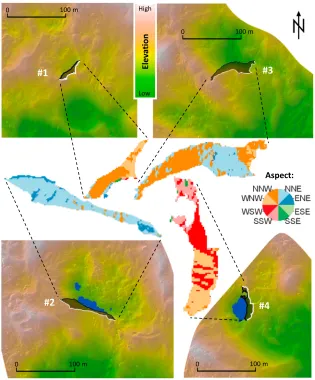
We investigate four ice cliffs on the debris-covered Lirung Glacier in the upper Langtang Valley, Nepalese Himalaya (28.232∘N, 85.562∘E; Figure 1), using aerial and terrestrial surveys of cliff geometry at the beginning and the end of the ablation season, which in this monsoon-dominated area approximately corresponds to the monsoon season. The cliffs, indicated as cliffs 1–4, range between∼4060 and 4200 m above sea level (asl) on the lower tongue of Lirung Glacier (Figure 1).
Two sets of high-resolution orthoimages and DEMs from UAVs were produced by SfM photogrammetry, cov-ering the lower part of Lirung Glacier [Immerzeel et al., 2014]. The two UAV-DEMs from 19 May and 22 October 2013 were originally produced at 0.2 m resolution and aggregated to 0.6 m because of the model’s computa-tional costs and numerical stability. They were used to derive the initial and final topography of the cliffs and the surrounding glacier surface, respectively. Selected UAV-DEM raster cells near cliffs 2 and 4 had unrealistic increased elevations due to water surface reflection in the May observations and were corrected manually by considering the local slope.
The outlines of the cliffs and nearby ponds were manually digitized from the UAV orthoimages, which have a spatial resolution of 0.1 m. Elevation models based on a triangulated irregular network (TIN) derived from UAV photogrammetry [Brun et al., 2016] are used for validation of modeled volume losses.
Figure 1.Overview of the tongue of Lirung Glacier, in the upper Langtang Valley, Central Nepalese Himalayas, based on a SPOT6-orthoimage from April 2014. The May UAV-DEM coverage is indicated in blue and the four investigated cliffs in yellow. The AWS sites are marked by a red triangle.
radiation (perpendicular to the surface), relative humidity of the air, wind speed, and air temperature (shielded and ventilated), all at a screen level of 2 m. Details about the sensor setup are provided inSteiner et al. [2015]. Debris surface temperature was measured, shielded from sunlight, on a rock at the station [Steiner and Pellicciotti, 2016]. Incoming longwave radiation was not measured at the AWS on the glacier and was therefore modeled with data from an AWS in Kyanjing (3857 m asl) about 2 km south of Cliff 1 (see Figure 1), following Steiner et al.[2015] andBuri et al.[2016]. Details of the modeling approach are provided inSteiner et al.[2015].
Some of the parameters used in the energy balance calculations are difficult to measure in the field (albedo for ice and debris, as well as surface roughness length) and were optimized inSteiner et al.[2015] and used as described inBuri et al.[2016]. These parameters were assumed to be uniform across the cliffs and constant in time.
3. Field Observations of Cliff Changes
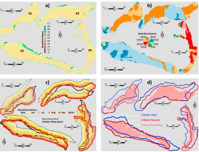
Figure 2.Aspect (insets) and elevation within 200 m×200 m area of interest (maps) for each cliff (1–4) based on the May 2013 UAV-DEM. On the maps the two-dimensional shape of the cliffs (dark area) is indicated by lines, with the white line marking the crest of the cliffs and the black line their base. Blue areas indicate ponds (pond at Cliff 3 not visible due to small size). The map background shows colors relative to elevation topped by hillshade.
aspect distribution and the cliff areas and dimensions (Figures 2 and 3 and Table 1) in May and October as derived from the high-resolution UAV-DEM for the four cliffs. We then use them to identify different cliff types in terms of geometry and evolution.
3.1. Reclining Cliffs
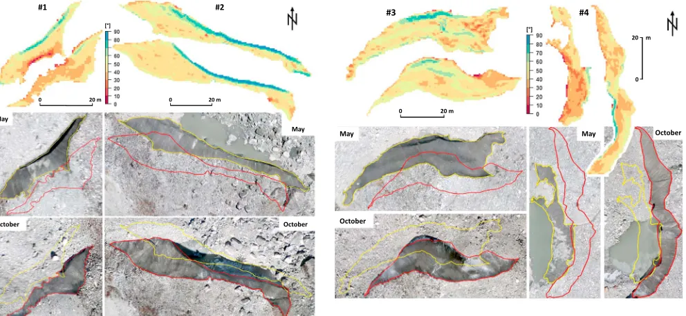
Cliff 1 is the smallest of the four surveyed cliffs and presented steep slopes at its base in May 2013 (Figure 3). No pond was present in May 2013 (Figure 2), although the steep lower section (see slope and orthoimage in Figure 3) indicates a probable former pond connection which likely disappeared before the field visit and the UAV flights in May 2013 [Brun et al., 2016]. A small adjacent pond could be identified on two Google Earth satellite images from postmonsoon 2011 (27 September and 5 October, respectively), in contact with the cliff section showing the steepest slopes in May 2013.
Cliff 1 reclined during the 2013 monsoon season, as indicated by markedly lower slope values, especially at the cliff base (Figure 3 and Table 1). Its area slightly diminished (Table 1) and shape changed (Figure 3), but the more striking transformation is the flattening of slopes.
Figure 3.Slopes derived from the UAV-DEM and manually delineated outlines of the four cliffs in May (top or left raster; yellow line on orthoimage) and October (bottom or right raster; red line on orthoimage) 2013, used as initial conditions for the model. Note the different scale bars for different cliffs.
played a negligible role. The area of the cliff decreases slightly (Table 1). Cliff 3 is the only cliff which slightly alters its main orientation between May and October, from overall NNW aspect to predominant NNE (Table 1).
The flattening of both Cliffs 1 and 3 is not entirely apparent from comparison of their mean slopes between May and October, as changes in area also play a role in the averaging of single cell slopes into a mean cliff value. A clearer signal of the general reclining can be found in the reduction of the cliffs’ vertical extent (Table 1) by 25.5% (Cliff 1) and 16.9% (Cliff 3). Both cliffs show a decreased inclined area in October, as a consequence of the removal of steep sections from the cliffs’ bases. Additionally, the slopes behind the two cliffs in the direction of backwasting are characterized by a depression downglacier (Figure 2) so that the cliff’s top ridge is lowered as a result of reduced ice volume for backwasting [Brun et al., 2016]. This leads to a slope reduction at the upper portion of the cliff that progressively decreases the cliff area.
3.2. Persistent Cliffs
Cliff 2, the largest of the four cliffs, maintains a remarkably consistent area and self-similar geometry from May to October (Table 1 and Figure 3). Adjacent to the main section of the cliff a pond is present both in May and in October 2013 (see Figure 3).
The decrease in mean slope toward October is due to the slight flattening of a steep section at the eastern top part. Through the fall of a large boulder the shading of the uppermost cliff part was stopped at one point in the period between the observations. The vertical extent is very similar between May and October, fur-ther suggesting that the cliff geometry has remained self-similar while backwasting (Table 1 and Figure 11).
Table 1.Cliff Characteristics Derived From the UAV-DEM and Orthoimage, Shown as Mean Values for 18 May and 22 October 2013, Respectivelya
Elevation (m asl) Aspect (deg) Slope (deg) Vertical Extent (m) Horizontal Extent (m) Area (m2)
Cliff # May Oct May Oct May Oct May Oct May Oct May Oct
1 4066.4 4061.7 328.3 (NNW) 316.9 (NNW) 46.8 43.5 14.5 10.8 47.4 46.1 297.5 251.8
2 4092.2 4092.2 29.8 (NNE) 31.8 (NNE) 53.0 48.4 23.7 24.7 100.7 95.6 1107.9 1113.3
3 4161.2 4155.5 358.9 (NNW) 3.1 (NNE) 49.7 48.5 33.1 27.5 82.3 72.6 1303.6 990.9
4 4201.5 4204.7 263.7 (WSW) 258.8 (WSW) 42.2 44.0 14.7 23.7 60.4 82.4 505.0 757.8
aFor elevation, the maximum value within each cliff area is taken. Aspect is defined from 0 to 360∘, with north at 0∘(vectorial mean). Values of vertical extent
[image:5.612.36.576.628.707.2]The backwasting pattern is uniform, and we know from water level records that the pond first filled slightly and then drained gradually.
3.3. Expanding Cliff
Cliff 4 is the only cliff which increases noticeably in area between the two observations (Table 1 and Figure 3), mainly due to its initial negative planform curvature in May 2013 (see aspect in Figure 2). Both vertical and horizontal extents increase in a pronounced manner from May to October, by 61.2% and 36.4%, respectively (Table 1). Slopes at the base of the cliff become steeper (Figure 3d), and the average slope increases by 1.8∘ (Table 1).
Although a pond is in contact with the cliff in both May and October, the cliff shape changes markedly dur-ing the melt season as a result of the draindur-ing of the pond, which lowers by about 6 m (calculated as a net change in elevation between the two DEMs). In addition to the increase in area, the most striking change in the geometry of this cliff is the reversal of slope patterns: the base of the cliff in contact with the water has generally shallow slopes in May, while in October the cliff zones at the pond shore are the steepest. In May, on the other hand, the steepest sections were located at the top of the cliff, in its central section. It is possi-ble that steep slopes at the base were also present in May but covered by the higher pond level and became exposed in October with the lowering of the water level.
3.4. Summary of Observed Cliff Types
To summarize, three categories of cliff behavior can be identified in terms of geometry, evolution, and pond coupling:
1. Absence of pond contact permits flattening of the cliff and causes continuous cliff reclining. 2. Consistent pond presence leads to steep sections at the cliff base, enabling a stable cliff geometry. 3. Lowering pond water level reveals steep formerly submerged ice in a cliff that grew radially in size.
Due to our restricted sample size, these cliff types might not be representative of the full variety observed at larger scales, on different glaciers, or in distinct climatic regimes. Assessing the dominant processes and changes for a larger sample of cliffs and for different locations will be a necessary future step for understanding the dynamics and relevance of ice cliffs.
4. Modeling Cliff Evolution
The patterns of cliff evolution observed on Lirung Glacier and described in section 3 cannot be explained by considering a static cliff geometry and by applying atmospheric melt alone [Buri et al., 2016]. From field evi-dence and qualitative results from the pioneering early studies on debris-covered glaciers in the Himalaya [e.g.,Iwata et al., 1980;Sakai et al., 1998], as well as from results of very recent works, it is evident that cliffs are moderated by the presence of supraglacial ponds at their base [Röhl, 2008;Miles et al., 2016]. Ponds were also observed to affect retreat of ice-cored moraines located at glacier termini in St. Elias Mountains (Canada) and in Vestfold Hills (Antarctica) [e.g.,Driscoll, 1980;Watson, 1980;Pickard, 1983]. Field observations sug-gest that ice reburial by debris can considerably affect cliff geometry and area [Thompson et al., 2016]. The inaccuracy of the static approach is exemplified by calculating only melt due to the interaction with the atmo-sphere (Figure 4). With the grid-based model that considers a static geometry where the cliff geometry is only updated once at the end of the melt season (hereafter referred to in short as “static model” and indicated as “S Model” [Buri et al., 2016]), the patterns of aspect (Figure 4a) and slope (Figure 4b) after one melt season are not realistic. This is mainly due to the long period before an update to geometry and hence long melt vectors that can intersect each other. Along with evidence from the field, this prompted the development of the new model presented here, which is dynamic in the sense that regular updates of the cliff geometry are conducted on the base of the high-resolution ablation calculations. We also represent two key processes observed in the field that seemed to affect cliff geometry and dynamics: (a) the presence of ponds and (b) reburial of lateral cliff sections by adjacent debris.
4.1. Model
Figure 4.Modeled (S Model) (a) aspect and (b) slope for Cliff 2 for October 2013 without considering intermediate geometry updates but only a final melt translation resulting from energy exchange with the atmosphere at the end of the melt season.
A daily geometry update was unreasonable for two reasons: computational costs and a geometry update distance less than the grid size, as typical daily melt rates at the cliffs surface are at the order of<10−1m.
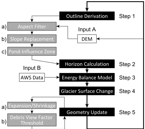
The model is coded in the open-source software R [Core Team, 2015] and is run separately for each cliff using the UAV-DEM of 0.6 m resolution. In the following, we explain the single modeling steps inside the D Model (Figure 5).
4.1.1. Cliff Outline Derivation (Step 1)
The outline of the ice cliff is needed as input to initialize the model, enabling separation of debris-covered and debris-free area in the calculations. Using the true-color georeferenced UAV orthoimage from May 2013,
[image:7.612.254.493.492.705.2]supported by terrestrial photography and experience from the field visits, cliff and pond outlines are derived manually. The latter are used to identify the pond-affected zones of a cliff (step 1c).
After each geometry update (step 5, section 4.1.5) the new cliff polygon is derived automatically to run the model on the new geometry. As a result of the different aspects (and therefore melt directions) the applica-tion of the melt vectors to each cliff cell can lead to voids between the translated cliff raster. The term “melt vector” describes the melt distance in combination with the three-dimensional melt direction per cliff cell. To avoid gaps within the updated cliff, the new outline is based on a convex-hull approximation, the alpha shape method [Edelsbrunner et al., 2006]. This approach draws a connected line around the updated cliff raster using a chain of circles approximating the cliff shape as closely as possible. The radius of the alpha shape circles is set to 3 times the resolution, i.e., 1.8 m. This size provides the best results in terms of penetrating into gaps between cells and not splitting the cliff into multiple polygons. The model internally increases this radius in case the cliff polygon is split, until a closed shape is reached again. In this way the model is avoiding dividing the cliff into multiple areas. As a consequence of the alpha shape method, the new cliff outline can increase in size compared to the previous polygon but can also shrink if transferred cells fall into the same cell after melting. Since these overlayed cells usually do not have the same elevation, a vertical discontinuity can occur with more than one elevation value per cell. If this happens, the minimum of the layered cell elevation values is taken and assigned to the cell.
In this study the DEM which is updated after model step 5 is referred to as the “active DEM.” By masking it with the cliff polygon, the geometry of the cliff surface can be extracted. In the initial model run, the UAV-DEM from May 2013 serves as input, while in every subsequent interval the active DEM is used. Slope and aspect are derived for every cell together with its elevation from the active DEM based on the algorithm ofHorn[1981] for rough topography using eight neighbors with differential weights and excluding the central cell itself. Marginal raster cells can be represented erroneously in terms of slope and aspect, as they can be influenced through the Horn algorithm by adjacent debris cells. To avoid these edge effects, we perform two steps (a and b below) to obtain a stable and realistic initial geometry for the ablation modeling.
Aspect filter (step 1a). A median filter with a window of size 9×9cell (29.16 m2) is applied to all aspect values
within the cliff area in order to (1) remove lateral edge effects at the transition of ice to debris along the cliff outline and (2) smooth out the high aspect variability of the active DEM, which is partly due to small inaccura-cies in steep terrain. The filter is needed to avoid calculation of an incorrect melt direction, as the melt vector depends partly on the aspect of a cliff cell.
Slope replacement (step 1b). A threshold of 40∘is applied to distinguish between debris-covered (<40∘) and potentially debris-free cells (≥40∘). The threshold has been determined from field and satellite measurements byFoster[2010] on Miage Glacier. Although maximum angles at which loose material can remain on inclined ice surfaces might vary depending on thickness and shape of debris [Reid and Brock, 2014], ice-exposed slopes <40∘were measured only rarely on supraglacial cliffs on the tongues of both Lirung [Steiner et al., 2015] and Langtang Glacier in 2013 and 2014 (unpublished). Unrealistically low slopes on the cliff surface, which were apparent especially at the cliff edges, would produce steep melt vectors pointing downward almost vertically. To avoid this effect, all cliff cells below the slope threshold were set to 40∘.
Pond influence zone (step 1c). The presence of supraglacial ponds seems to have an important effect on ice wall evolution [Driscoll, 1980;Watson, 1980;Pickard, 1983;Miles et al., 2016;Buri et al., 2016;Brun et al., 2016]. Two horizontal buffers are applied to define a potential influence zone on the ice cliff surface. The first one is applied to search for all cliff raster cells lying within a 1 m band around the pond shore, while the second buffer identifies cliff cells with a slope≥60∘at a maximum distance of 5 m from the pond outline. The two resulting groups of cells are merged to a pond influence zone, where an enhanced melt rate is added to the horizontal melt component derived from the atmospheric energy balance (step 3). This extra melt accounts for subaqueous melt and is taken equal to 0.033 m d−1. This is the mean value calculated byMiles et al.[2016]
in their energy balance study of a pond (at Cliff 2) on Lirung Glacier during monsoon 2013. Calving, although observed at other field sites [e.g.,Inoue and Yoshida, 1980], is unlikely to occur for these cliffs since the ponds are small [Sakai et al., 2009].
4.1.2. Horizon Calculation (Step 2)
Emission and Reflection Radiometer global DEM 2) (for distal topography) with a resolution of 1 arc sec (∼30 m) [Tachikawa et al., 2011], followingSteiner et al.[2015] andBuri et al.[2016]: the active DEM, adapted after each geometry update, is used to describe the close topography within a 200 by 200 m grid (Figure 2), while the ASTER-GDEM2 is used for the rest of the glacier surface and distant mountain ridges for calculation of shading [seeBuri et al., 2016, Figure 4]. Details of all calculations are provided inBuri et al.[2016].
4.1.3. Energy Balance (Step 3)
The view factors and horizon angles calculated in step 2 are used in the surface energy balance model for a fully distributed calculation of the radiative fluxes.
The energy balance at the cliff surface is
Qm=In+Ln+H+LE, (1)
whereQmis the energy flux available for melt,InandLnare the net shortwave and longwave radiation fluxes,H
is sensible heat, and LE is latent heat flux. All fluxes are perpendicular to the surface and expressed in W m−2.
The heat from precipitation and conductive heat flux into the ice are neglected [Reid and Brock, 2014]. The surface energy balance for each cliff cell is computed using hourly meteorological data followingBuri et al. [2016]. The model is run from 19 May to 22 October 2013 (dates of the UAV data acquisitions).
4.1.4. Glacier Surface Change (Step 4)
While ice cliffs backwaste several meters over a single melt season [Brun et al., 2016], the debris-covered glacier surface also slowly changes due to subdebris melt and glacier flow. The relevant glacier dynamics are consid-ered in the model by using tie points, which are detectable objects visible in both UAV orthoimages in May and October 2013. Large boulders serve as tie points and define stable references on the glacier during this period. Based on a distributed tie point approach [Immerzeel et al., 2014], a thin plate spline interpolated map of displacement was created. Because the tracked boulders lie on the debris-covered parts of the glacier, the differential ablation occurring at ice cliffs does not affect the interpolation. The resulting map provides verti-cal and horizontal surface changes for every grid cell on the stable glacier surface. The vertiverti-cal glacier change is applied to the active DEM together with the monthly cliff shape recalculation. The horizontal surface move-ment is not considered in the model but used to correct the observed October cliff outlines (Figure 8) for the glacier surface displacement from May to October 2013. Vertical and horizontal shifts are very small on Lirung Glacier with mean daily changes of−0.0049 and 0.0072 m d−1, respectively.
4.1.5. Geometry Update (Step 5)
In the last model step the cliff geometry is updated according to the melt of ice per cliff cell,dmelt(m), resulting from the energy balance calculations in step 3 accumulated over each month:
dxy=dmeltsin𝛽, dz=dmeltcos𝛽 , (2)
dx=dxysin𝛾, dy=dxycos𝛾 , (3)
wheredzanddxy(m) are the melt distances in vertical and horizontal directions, respectively. The latter is the
resulting vector of the horizontalxandycomponents,dxanddy, respectively. The angles𝛽and𝛾indicate
slope and backazimuth (𝛾= azimuth−180∘) of the cliff cell, respectively (Figure 6).
The new cliff raster cannot be simply embedded into the glacier-wide active DEM, as the updated cells are now located at a different position due to backwasting. The horizontal melt vectors are used to remove relict topog-raphy from the former cliff position. The elevation of the cells overlaid by the melt vectors were interpolated linearly between the starting and ending points of the melt vector.
Figure 6.Schematic cross section of cliff backwasting from left to right (step 5). All cliff edges which are visible from the reader’s point of view are shown as solid lines; hidden lines are dashed.
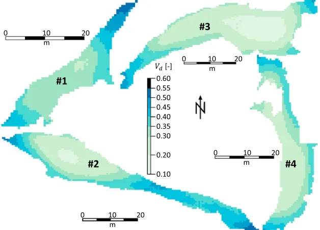
Debris view factor threshold. Unrealistic cliff outgrowths are limited in the model by the application of a sky view factor threshold. Lateral outgrowths of the cliff surface, unrealistically directed toward and cut into debris slopes, are often not automatically removed by the slope threshold described above. To contain these incorrect instances of expansion, cliff cells with high debris view factors (Vd>0.45) are converted into
debris-covered cells. The threshold is assumed to be equal for all cliffs and selected according to test runs with the most realistic results.Vdcan be regarded here as a measure of how deep a cliff is cut into a debris
ramp. Therefore, usingVdas a parameter to control cliff expansion has a clear physical meaning, as above the
critical value the portion of debris seen by a cliff cell exceeds 45% of the total surrounding area (i.e., less than 55% is defined as sky or ice), which makes reburial by surrounding rocks or melt-out by extrahigh longwave
Figure 7.Modeled debris view factors (Vd) for each cliff (1–4) calculated from the initial UAV-DEM in May. Cliff cells with
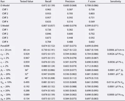
[image:10.612.218.532.485.711.2]Table 2.Validation Metrics and Results of the Sensitivity Analysis for Different Model Runs (Listed in the First Column)a
Run Tested Value Recall Precision Fscore Sensitivity
D Model 0.872 (0.139) 0.600 (0.068) 0.708 (0.086)
Cliff 1 0.965 0.587 0.730
Cliff 2 0.933 0.705 0.803
Cliff 3 0.957 0.592 0.731
Cliff 4 0.633 0.516 0.569
S Model 0.807 (0.057) 0.480 (0.079) 0.599 (0.071)
Cliff 1 0.726 0.382 0.501
Cliff 2 0.846 0.600 0.702
Cliff 3 0.873 0.448 0.592
Cliff 4 0.784 0.488 0.602
PondOff 0.874 (0.152) 0.587 (0.075) 0.699 (0.094)
rs + 20 cm 80 cm 0.730 (0.141) 0.627 (0.122) 0.667 (0.104) 0.0006ΔF/cm rs
𝜖d−2% 0.929 0.872 (0.137) 0.594 (0.082) 0.704 (0.086) 0.0026ΔF/%𝜖d
𝜖d+2% 0.967 0.875 (0.131) 0.578 (0.078) 0.693 (0.087)
𝜖i−2% 0.959 0.876 (0.125) 0.581 (0.079) 0.698 (0.083) 0.0036ΔF/%𝜖i
𝜖i+2% 0.996 0.880 (0.124) 0.602 (0.074) 0.712 (0.082)
𝛽T−10% 36∘ 0.905 (0.086) 0.559 (0.077) 0.688 (0.068) 0.0001ΔF/∘𝛽T
𝛽T−20% 32∘ 0.947 (0.029) 0.536 (0.082) 0.681 (0.065) 0.0001ΔF/∘𝛽T
𝛽T+20% 48∘ 0.743 (0.208) 0.632 (0.112) 0.679 (0.153)
Vd
T+10% 0.495 0.881 (0.161) 0.533 (0.069) 0.661 (0.090) 0.0116ΔF/%VdT
𝛼i−20% 0.192 0.885 (0.132) 0.583 (0.088) 0.700 (0.090) 0.0001ΔF/%𝛼i
𝛼i+20% 0.288 0.874 (0.165) 0.583 (0.063) 0.698 (0.095)
𝛼d−20% 0.089 0.878 (0.139) 0.584 (0.082) 0.698 (0.085) 0.0000ΔF/%𝛼d
𝛼d+20% 0.134 0.873 (0.127) 0.584 (0.075) 0.697 (0.083)
aThe values are averaged over the four cliffs from May to October. For D and S Model runs the metrics for each cliff
are shown additionally. Standard deviation among cliffs is shown in parentheses. Except for the S Model run, all runs are based on the D Model with a single parameter changed at a time. In run “PondOff” the pond influence algorithm was suppressed. In run “rs” the spatial resolution of the UAV-DEMs was altered, in𝜖iand𝜖dthe emissivities of ice and debris, respectively, were changed. “𝛽T” and “Vd
T” indicate the runs where the threshold values for slope and debris view
factor were modified,𝛼iand𝛼dthe runs where ice and debris albedo were changed. The second column shows the value corresponding to each specific run. The metrics Recall, Precision, andFscore are described in section 4.2. Sensitivity is shown as change in theFscore (ΔF) per unit change of the corresponding parameter.
radiation likely. Figure 7 shows the distribution ofVdas modeled for the initial cliff shapes in May 2013. As described above, all cliff cells above the threshold are considered to be covered by debris by the end of each model interval and no volume loss is assigned to these areas.
4.2. Validation Metrics
We validate the model by comparing observed and modeled cliff dimensions, slopes, and aspects, as well as comparing the calculated volume losses to those derived from a TIN-based calculation inBrun et al.[2016]. Direct comparison of the observed and modeled area is not very meaningful, as the same single absolute surface area value could correspond to two different cliff shapes and locations. To take into account the areas that are correctly identified by the model, we calculate metrics that are commonly used in image classification and segmentation for binary images. We define three possible outcomes when identifying a cell as belonging to a cliff or not: (1) true positive (TP), when a cell is correctly detected as cliff by the model; (2) false positive (FP), when a cell is erroneously modeled as cliff; and (3) false negative (FN), when a cell is modeled as debris but in reality is part of a cliff. Using TP, FP, and FN, we then define the following common metrics [e.g.,Olson and Delen, 2008;Rittger et al., 2013]:
Precision= TP
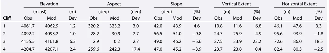
Table 3.Cliff Characteristics Derived From the UAV-DEM (“Obs”) and Modeled With the D Model (“Mod”)a
Elevation Aspect Slope Vertical Extent Horizontal Extent
(m asl) (m) (deg) (deg) (deg) (%) (m) (%) (m) (%)
Cliff Obs Mod Dev Obs Mod Dev Obs Mod Dev Obs Mod Dev Obs Mod Dev
1 4061.7 4062.9 1.2 320.2 323.2 3.0 42.0 43.9 4.6 10.8 11.6 6.8 46.1 47.6 3.3
2 4092.2 4093.2 1.0 28.2 30.9 2.7 56.5 51.0 −9.8 24.7 25.9 4.9 95.6 93.9 −1.8
3 4155.5 4161.8 6.3 2.9 0.2 2.7 49.0 46.2 −5.6 27.5 33.9 23.2 72.6 86.0 18.5
4 4204.7 4207.1 2.4 259.6 242.3 17.4 47.0 45.2 −3.9 23.7 23.8 0.4 82.4 80.3 −2.5
aThe mean values are shown together with the respective deviations for 22 October 2013. For elevation the maximum value within the cliff area was taken.
Aspect values (vectorial mean) are defined from 0 to 360∘with north at 0∘. Mean aspect and slope values are weighted with the inclined area of each cliff cell. Values for vertical extent indicate the highest difference in elevation within the cliff area; horizontal extent shows the manually defined maximum straight distance within the cliff outline.
Recall= TP
TP+FN, (5)
F=2⋅ Precision⋅Recall Precision+Recall=
2⋅TP
2⋅TP+FP+FN. (6)
Precision measures the probability that a cell detected as cliff by the model indeed is cliff [Rittger et al., 2013], and Recall is the fraction of real observed cliff area that was correctly detected in the model and shows the probability of detection [Dong and Peters-Lidard, 2010].F(Fscore or Dice coefficient), a measure of segmenta-tion agreement, balances Precision and Recall by penalizing both missing cliff cells and falsely detected debris as cliff [Dice, 1945;Gilani and Rao, 2009;Rittger et al., 2013]. It ranges from 0, indicating no spatial overlap between two sets of binary segmentation results, to 1, indicating complete overlap [Zou et al., 2004].
4.3. Model Sensitivity
Since several of the model parameters are evaluated on individual tests, by trial and error or taken from the literature, we perform a sensitivity analysis to evaluate their importance to the model outputs (Table 2). Assuming as reference the D Model run with the setup described in section 4, we vary each parameter one at a time by a given amount (chosen based on field experience or from the literature) and calculate the corre-sponding Recall, Precision, andFScore. We also evaluate the metrics for the S Model run and for a run where the pond influence is turned off. The varied parameters are spatial resolution of the UAV-DEMs, emissivities of ice and debris, threshold values of slope, and debris view factor, as well as ice and debris albedo.
We evaluate the sensitivity of the model to changes in the parameters by calculating the change inFscore per change of parameter unit (i.e., degree or percentage).
5. Results
In this section we compare D Model results to the observed October surface. The S Model simulations are also presented for comparison. First we focus on cliff dimensions, slope, and aspect, then we investigate time series of radiative fluxes for each cliff and recorded meteorological data to explain differential patterns of cliff changes. Finally, the calculated volume loss and melt rates per cliff are compared to validation data and model sensitivities are briefly discussed.
5.1. Dimensions, Slope, and Aspect
The evolution of the four cliffs in terms of slope, aspect, and outline is shown in plan view in Figure 8 and as profile for Cliff 2 in Figure 11. Cliff geometry and dimensions, modeled and observed, are listed in Table 3. 5.1.1. Cliff 1
Figure 8.Model results of (a) slope and (b) aspect for October 2013 for each cliff (1–4). (c) The simulated cliff evolution based on the monthly updated outlines (D Model); for comparison the May and October observations are shown in the background. (d) The October cliff outlines simulated with the D Model (red) and the S Model (blue), respectively. The rose area in the background indicates the observed cliff area from the October UAV orthoimages.
The cliff outline, and the magnitude of the backwasting, is also reproduced well by the model with the excep-tion of the lateral secexcep-tions. The modeled outline along the top (south) and base (north) of the cliff agrees well with the observed shape, but the lateral margins are not accurately reproduced. The western corner sees a larger area than observed, whereas the eastern corner is partly removed (Figure 8a).
Comparison with the output of the S Model (Figure 8d) shows that for this cliff it is crucial to account for the dynamic processes included in the D Model, and the S Model is not able to reproduce the position of the cliff base, with less backwasting at the base but also an overestimation of the cliff area in its topmost sections. 5.1.2. Cliff 2
The agreement between modeled and observed geometry is very good for Cliff 2, and the self-similarity of the May and October geometry (Figures 3) is reproduced well by the model in terms of outline and slope distribu-tion (Figures 8 and 11). The steep lower secdistribu-tion, a principal characteristic of Cliff 2 in both May and October, is present also in the modeled cliff shape, even though some discrepancies are evident. The D Model simu-lates the average slope (51∘) with a deviation of−5.5∘or 9.8%, the highest among all cliffs. The modeled cliff dimensions agree very well, with a small discrepancy of 1.2 m (vertical) and−1.7 m (horizontal). The average modeled aspect agrees with the average observed aspect (with a difference toward east of 2.7∘).
The average backwasting is well reproduced, and the cliff base and its top are simulated in the correct location. This is apparent also for the S Model in the central section of the cliff, but a main deficiency when using the S Model is a distinct outgrowth of ice at the eastern margin and a similar remnant in the northwestern section. 5.1.3. Cliff 3
Figure 9.Daily mean values of (a–d) modeled (D Model) radiative fluxes (W m−2) averaged over each cliff and
(e) measured temperatures (∘C) at AWS Lirung. SW dir, direct shortwave radiation; LW deb, longwave radiation coming from surrounding debris; net SW and net LW, net shortwave and longwave radiation (incoming minus outgoing flux). For shortwave fluxes only the hours between 8:00 and 17:00 (in Nepal Time, UTC+5:45) were considered.
is simulated by the D Model in a satisfying manner (Figure 8), even though the overall deviation in average slope is, at−2.8∘.
The overall backwasting of the cliff is reproduced well, with very high agreement at the cliff top and good agreement at the (steep) central basal part (Figure 8c). However, discrepancies are evident at the sides, where the ice-debris boundary does not backwaste enough in the model. Both the eastern and western marginal portions of the cliff are preserved in shape by the D Model, but observations show that they shrank and migrated farther south (Figure 8c). The model thus results in an overestimation of area. These effects are more pronounced in the S Model simulations (Figure 8d), which overestimate the ice cliff surface considerably at the margins but also in the region along the cliff base. The simulated dimensions (D Model) exhibit the high-est discrepancies to the observations of the four cliffs (23.2% for the vertical and 18.5% for the horizontal dimension) because of the errors at the margins. The difference in modeled (D Model) and observed mean aspect is instead very small (2.7∘, Table 3), because the bulk of the cliff geometry is preserved.
5.1.4. Cliff 4
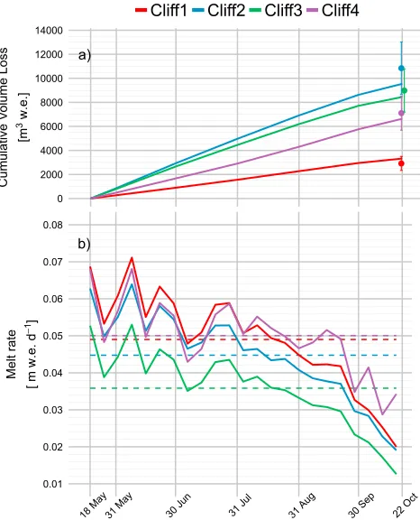
Figure 10.(a) Modeled cliff volume losses from May to October shown as lines, compared to the TIN-generated volume losses (points) with their error bar of±20%, as estimated inBrun et al.[2016]. (b) Modeled daily melt rates (solid lines), averaged per cliff and obtained as the weekly average, and May to October mean cliff melt rates per cliff (dashed lines).
can be recognized. In addition, the elongated dent pointing to the west that is evident in the observations in May is maintained by the model during the cliff backwasting, whereas it disappears in reality (Figure 8c), likely reburied by debris.
The overall slope simulated by the D Model deviates by−1.8∘from the observation, the average aspect by 17.4∘toward west. Another failure of the model is in the steeply sloped lower section of the cliff (section 3) which the model cannot replicate.
5.2. Radiative Fluxes
Cliff 4 receives the highest amount of direct (SW dir, Figure 9) and net (net SW) shortwave radiation of all cliffs throughout the melt season and in particular in September and October. In this period, the direct solar radiation received by Cliff 4 is more than double the amount for Cliffs 1 to 3. This distinct pattern is also evident in the net shortwave radiation. Differences in longwave radiation from the surrounding debris (LW deb) and the total net longwave income (net LW) are less pronounced but still important. Cliff 1 receives the highest longwave radiation throughout the simulation period, and Cliff 3 the lowest. This can be explained by the debris slopes facing Cliff 1 at close distance, as indicated by high debris view factors in Figure 7 (0.35 on average). In contrast, Cliff 3 sees a smaller portion of surrounding debris (0.26 on average).
In general, all fluxes in Figure 9 show a reduced temporal variability during monsoon season (mid-June to beginning of September). Measured air and surface temperatures are also reduced in their variability during this period and differ less compared to premonsoon and postmonsoon.
5.3. Volume Loss, Melt Rate, and Area
Simulated volume losses and melt rates from May to October 2013 calculated with the D Model are shown in Figure 10 and Table 4. Model results are compared to the volume losses derived from high-resolution cliff geometry obtained with SfM as TIN inBrun et al.[2016]. Note that the TIN results ofBrun et al.[2016] are provided as volume of ice but were modified to m3w.e. (water equivalent) for comparison, using an
assumed ice density of 900 kg m−3. The cliff outlines in premonsoon and postmonsoon which serve as base
Table 4.Ice Cliff Volume Loss (m3w.e.) and Mean Backwasting Rate (m w.e. d−1) From May to October 2013 for the Four Cliffsa
Volume Loss Melt Rate
(m3w.e.) (%) (m w.e. d−1)
Cliff # Obs. Mod. Dev. Mod.
1 2,917.3 (2,333.8–3,500.8) 3,325.6 14.0 0.048
2 10,845.1 (8,676.1–13,014.1) 9,544.4 −12.0 0.040
3 8,987.0 (7,189.6–10,784.4) 8,447.6 −6.0 0.033
4 7,110.4 (5,688.3–8,532.5) 6,634.9 −6.7 0.051
aModeled volume losses (Mod., D Model) are compared to the TIN-derived (Obs., based onBrun et al.[2016]) volume
loss, together with the relative deviation (Dev.) between the modeled and observed values. The uncertainty range of ±20% estimated inBrun et al.[2016] is indicated in parentheses. Mean backwasting rates obtained as volume loss divided by the corresponding area are also provided.
Therefore, the volume losses from the TIN approach should be used as a reference rather than an exact validation. The uncertainty range of±20% estimated inBrun et al.[2016] is also indicated in Figure 10a.
Simulated volume losses all agree with the TIN-derived values within the given uncertainty ranges (Figure 10a and Table 4). Estimated volume losses are smaller than the ones ofBrun et al.[2016] for all cliffs except Cliff 1 (Table 4).
Volume losses at the end of the study period are an integrated variable of cliff backwasting processes. The daily melt rates averaged over the entire cliff area and to weekly values, calculated as melt amount multiplied with inclined area per cell, provide a better insight into temporal patterns of changes (Figure 10b).
The melt rates at all four cliffs show a clear reduction toward the end of the melt season with distinctly lower values in postmonsoon. Melt rates at Cliffs 1, 2, and 4 are similar in magnitude until end of July, when melt at Cliff 4 becomes higher while it decreases at Cliff 2. The melt rate at Cliff 3 is remarkably smaller in mag-nitude (0.036 m w.e. d−1on average with a minimum daily melt rate among all cliffs of 0.013 m w.e. d−1by
mid-October), indicating that the high volume losses at this cliff (Figure 10a) is due to the larger area.
The highest melt rate is at Cliff 1 (0.071 m w.e. d−1) in early June before monsoon starts, but this cliff also shows
the highest variability during the melt season (0.051 m w.e.) as its melt rate goes down to 0.02 m w.e. d−1. The
highest mean melt rate over the entire period of record (May to October) is simulated for Cliff 4, with multi-ple postmonsoonal increases in melt rate (probably related to the exposure of west oriented cliff sections), whereas melt rates at the other cliffs decrease progressively from mid-September on. This behavior of Cliff 4 results in the lowest variability in melt rate (0.039 m w.e. d−1) among all cliffs.
From Figures 8c and 8d, it is apparent that the model overestimates the cliff area. Comparison of areas per se is not entirely meaningful, as the same total area could result from combination of erroneous cells identi-fied as cliffs together with cliff cells wrongly identiidenti-fied as noncliff. For this reason, we use more sophisticated validation metrics calculated for the projected area that account for the correctly identified cells (section 4.2). Table 2 shows that the D Model reference run has, on average over all four cliffs, a high Recall value (0.872), acceptable precision (0.600), and a highFscore (0.708). The latter is higher than in all other runs tested.
5.4. Model Sensitivity
The D Model run has the highest averageFscore value of all models (Table 2), which suggests that the chosen parameter values are an appropriate set. The S Model has the lowest value over the four investigated cliffs, confirming the poor performance of this model version (Figures 4 and 8d). The cliff where the D Model perfor-mance is worst in terms of Recall rate andFscore relative to the S Model is Cliff 4. This can be seen in Figure 8d, where the shift of the D Model outline toward east is apparent, which reduces prediction of observed cliff area and therefore lowers the Recall value. In turn, the precision is higher than with the S Model. Ignoring the effect of ponds adjacent to a cliff only slightly decreases theFscore value, as the main effect of a pond is on the cliff’s slope distribution rather than area.
32∘), but very few a higher precision (Table 2). As a result, none of the additional runs has a higherFscore than the reference run (0.708) except for the run with increased emissivity (0.712), which is only slightly higher.
The factor to which the model seems most sensitive, for the explored ranges, is the debris view factor thresh-old (“VdT”) used to rebury cliff cells that are surrounded by a large area of debris. The change in theFscore
(0.0116ΔF/%VdT) is at least 1 order of magnitude higher than the results from all the other runs.
The standard deviations of the scores (values in parentheses in Table 2) among the four cliffs are generally homogenous with only a small total range over all model runs. The standard deviations are highest for Recall (0.128) and lowest for Precision (0.082).
6. Discussion
6.1. Observations of Cliff Evolution
Out of four cliffs for which detailed, high-resolution observations were available, we noted three main patterns of evolution over the course of an ablation season, indicating a large variability that makes generalizations of cliff behavior difficult. It is clear that detailed observations for a longer duration and for a larger sample size of cliffs are needed to shed light with certainty on the principal processes. However, some key results emerge also from the analysis of four cliffs in this study.
The first is the presence and role of supraglacial ponds at the base of a cliff. The presence of supraglacial ponds adjacent to ice cliffs seems to be one of the main factors controlling whether a cliff flattens or is able to preserve a steep face (Figure 11). The pond maintains a steep cliff directly through thermoerosion or sub-aqueous melt at the pond-cliff interface and indirectly through exposure of the steep sections to increased longwave radiation emitted by the debris surrounding the cliff-pond system. Steep subaqueous ice slopes were observed with use of a sonar transducer on Lirung Glacier in 2013 (unpublished), which identified that maximum pond depth occurred immediately adjacent to the cliff-pond margin. Observations at other study sites have also revealed a steep subaqueous ice face [e.g.,Benn et al., 2001], which might not be the case with all pond-cliff systems but seems to be a frequent characteristic.
A second important factor controlling cliffs’ growth is related to reburial by debris. In the model this is accounted for in a twofold way, with a threshold slope under which debris-free cells are reburied and by a threshold for the debris view angle. Despite its simplicity, this approach works satisfactorily. From a combi-nation of model results and observations, this effect seems to be important at the cliff margins, and ignoring it will lead to overestimation of cliffs’ areas. However, this should not result in major discrepancies in vol-ume losses as these result mainly from melt occurring in the central section of the cliffs, as indicated by the fact that despite the overestimation of cliff areas by the model, the total volume loss is simulated correctly (Figure 10). Nevertheless, for modeling applications aimed at understanding future cliff evolution, inclusion of this aspect seems imperative to avoid unlimited areal growth which would translate into erroneous melt and backwasting patterns over the long term.
Observations also show a variety of aspects and shapes, and while none of the cliffs has a south facing ori-entation, it is remarkable that the only growing cliff was the west facing Cliff 4, which received much higher average radiative energy than the other three cliffs (Figure 9). We were not able to attribute this growth to aspect alone, but the distributed, high-resolution simulation of the radiative fluxes provides a clear indica-tion of higher energy receipts. This also highlights the importance of a grid-based, sophisticated model of energy fluxes.
6.2. Model Simulations
Figure 11.(top) Orthoimages showing the glacier surface in (left) May and (right) October 2013, with observed (orange solid) and modeled (yellow dashed) final Cliff 2 outlines. The corresponding debris-ice contact points are indicated with dots (using the same color scheme: orange for observations and yellow for model results). The two transects A and B (dark red dashed) are also shown. (bottom) Elevation profiles across Cliff 2 as observed in May and October (blue and green) and modeled from May (yellow) to October (red). The dots indicate the interfaces indicated in the orthoimages above (using the same color scheme: orange for observations and yellow for model results).
backwasting in the uppermost section of the cliff is reproduced very well by the model, and total volume losses agree with the observed values (Figure 10). For Cliffs 1, 2, and 4 simulated dimensions, slope and aspect patterns, and maximum elevations all agree well with the UAV observations, suggesting that the overall backwasting pattern is reproduced by the model.
Figure 12.Observed slopes at and around Cliff 3 in (a) May and (b) October are shown in the background. Thin and bold black outlines in the foreground show the observed cliff outlines in May and October, respectively. The red outline is the D Model result. White arrows indicate the ridge and dip direction of the main debris slope as a trace from cliff backwasting path. (c) A reason for the large overestimation of the modeled cliff area could be convergent accumulation of debris in the cirque sourcing from concave crests (red dashed line), which could not be considered in the model.
6.3. Model Limitations
Some of the approaches implemented in the model presented here are simple and could be improved toward more physically based formulations. The effect of an adjacent pond is included through prescription of a con-stant subaqueous melt rate and an affected area that was defined based on sensitivity tests. A more advanced approach could be devised based on the temperature of the pond water but would require data that are not easily available. Equally, the reburial by debris is parameterized as a function of slope and the amount of debris that is seen by any given cell of the cliff. A more accurate representation could be based on prescription of a source area and debris characteristics, but this also would imply knowledge of the geology of the debris and more burdensome calculations in a model that is already very complex. The main modeling goal that drove the formulation of the model was to incorporate first-order controls of cliff changes in a manner that would allow the model to be run for several cliffs and relatively long times without requiring too detailed or specific data sets.
A more stringent limitation related to the effect of ponds is the lack of knowledge about their hydrological variability and water levels. The reversal of slope observed at Cliff 4, with a flat lower cliff section in May turning into a steep one in October, was not reproduced by the model but could be explained by varying pond levels, which are not considered in the simulations. According to observations, the pond adjacent to Cliff 4 lowered substantially toward postmonsoon, exposing a newly steep section at the cliff base, where the pond most probably filled up in early premonsoon flooding the lower cliff zone.
The partial disagreement between the observations and modeled cliff geometry for Cliffs 1 and 3 might also be explained by the fact that between the two field visits of May and October 2013 the boundary conditions in the immediate vicinity of the cliffs changed significantly, most likely by the appearance of an ephemeral pond. In general, observations during monsoon and knowledge about pond evolution on debris-covered glaciers are very limited [Watson et al., 2016]. Therefore, it is difficult to make assumptions about potential interseasonal occurrence of supraglacial ponds and prescribe variable pond levels in the model. Neverthe-less, it is evident that comparison of model results with field observations can provide insights into processes occurring in the time between observations.
Another model limitation is related to some of the meteorological input data, which were applied in a nondis-tributed way: unlike the radiative fluxes, air temperature, relative humidity, and wind speed were assumed to be uniform in space. The point-scale AWS measurements were taken as such and uniformly applied to each cliff cell, because of lack of better methods for their extrapolation or modeling. Investigations into the microm-eteorology of high-elevation debris-covered tongues and Himalayan glaciers is, despite recent progress [e.g., Steiner and Pellicciotti, 2016;Collier and Immerzeel, 2015], a field still in need of sustained focus.
Surface parameters (surface roughness, and ice and debris albedo) were also assumed uniform in space. Despite the fact that they can show high spatial and temporal variability, these quantities are difficult to measure in a distributed manner at the cliff scale, for obvious logistic difficulties. Debris albedo depends on radiation patterns and shadow, precipitation determining the wetness of the surface, and debris properties. Ice reflectance additionally depends on preferential melt flow paths and amount of debris sources above the cliff as well as refreezing. Very little is known about surface roughness of cliffs and debris surfaces in general [Brock et al., 2010;Rounce et al., 2015]. For both albedo and surface roughness we used values optimized in Steiner et al.[2015] for Cliffs 1 and 2 where comprehensive survey data sets were available in both premon-soon and postmonpremon-soon 2013, but it is clear that a better understanding of the spatial and temporal variability of cliff surface properties could lead to improvements in modeling outputs.
The model seems to have problems in handling very thin, branching cliff segments, as could be seen in the modeled outlines of Cliff 4. This could lead to the development of incorrect cliff remnants with the wrong aspect, a problem that was small for Cliff 4 but could be more significant for other cliffs. As noted above, discrepancies in cliff areas would not necessary result in large errors in simulated volume losses as long as the areas are marginal, but depending on their main aspect they could represent a source of error over the long period.
6.4. Comparison With Other Studies
The development of the first grid-based model of cliff ablation that considered the cliff surface as a 3-D domain was a significant step forward [Buri et al., 2016]. This work shed considerable light on the spatial variability over a single cliff of the atmospheric forcing and quantified for the first time the relative importance of the various fluxes. However, that model includes only the atmospheric forcing (although in a distributed manner) and does not consider other processes that modulate the backwasting of a cliff and its geometrical changes. Here we show that updating the surface geometry is crucial for realistic calculations of the volume lost by a cliff during one ablation season and that a gridded representation of the cliff surface is necessary to quan-tify melt rates appropriately. We also show that accounting for melt at the surface of the cliff exposed to the atmosphere is only one of the processes that drive the dynamics of cliffs and their survival and decay.
Simulations with the new model provide an estimate of May–October mass losses from the four cliffs inves-tigated that range from 3326 (Cliff 1) to 9544 (Cliff 2) m3w.e. The contribution of the four cliffs to total
subdebris melt, estimated with an advanced glaciohydrological model [Ragettli et al., 2015], is 3.25%. This value is remarkable, given the small area ice cliffs cover relative to total debris-covered area (0.19%).
In a recent study on Ngozumpa Glacier, Everest region,Thompson et al.[2016] found that cliffs accounted for 40%of the volume losses over the stagnant portion of the glacier tongue by differencing of DEMs. It is difficult to compare these values to those obtained in our study, because the method used byThompson et al.[2016] often also included ponds in the area regarded as cliff, leading to high uncertainty. It would be useful to apply our model to all cliffs over a large glacier and compare those estimates to those ofThompson et al.[2016].
The new model could also be used to understand long-term patterns of cliff changes over several ablation sea-sons and employed to test hypotheses on cliffs survivals such as that only north facing cliffs (on the Northern Hemisphere) survive over multiple seasons that have been put forward but never demonstrated.
The model, however, given the level of complexity and physical detail included, might not be applicable as such at the glacier scale, for computational reasons and because it requires high-resolution DEMs of the cliffs and their surrounding topography that are rarely available for an entire glacier or catchment. For applica-tions at this spatial scale, for which only coarser-resolution DEMs are generally available, the effect of the DEM resolution on the accuracy of the model outputs needs to be tested.
7. Conclusions
In this paper, we have used a new data set of high-resolution observations of cliff evolution over one ablation season to identify patterns of changes over four cliffs on the debris-covered tongue of Lirung Glacier. The four cliffs have different shape, dominant orientation and slopes, and different degree and history of coupling to a supraglacial pond. We use the observations to infer the dominant processes controlling the observed evo-lution based on analysis of backwasting rates and cliffs’ geometrical properties. We then use the knowledge gained in this way to develop a model of cliff backwasting that takes existing models a step forward by includ-ing the cliffs dynamics in response to atmospheric forcinclud-ing (included to date), the effect of ponds at the cliff base, and reburial by debris. To our knowledge, this is the first model to move beyond theoretical ablation rates for an invariant surface and to represent 3-D evolution of cliffs.
Our main conclusions are as follows:
1. Out of four investigated cliffs, three different and contrasting patterns of evolution are evident. We show that cliffs on the same glacier and at short distance within each other can both flatten and recline, remain remarkably self-similar during one ablation season, or expand radially in a considerable manner.
2. We were able to identify some of the mechanisms controlling the patterns described above through a com-bination of high-resolution observations and an advanced model. In particular, we developed a model that accounts for the three main processes that seem to be first-order controls on cliff evolution: (i) atmospheric melt, (ii) pond contact ablation enhancement for the cliff base, and (iii) reburial by surrounding debris. 3. The modeling approach suggested is able to simulate the cliff evolution over one melt season in a satisfying
erroneous results in terms of backwasting patterns and volumes. Similarly, ignoring the effect of adjacent ponds or reburial by debris misses major factors affecting cliff evolution
4. Observations and model results suggest a strong dependency of the cliffs’ life cycle on supraglacial ponds, as the water body keeps the cliff geometry constant through a combination of subaqueous and atmospheric backwasting as well as calving at the base to maintain steep ice cliff slopes in the lowest sections. The absence of ponds causes the progressive flattening of the cliff, which finally leads to complete disappearance.
Despite the clear advances, several improvements are still possible and require high-resolution time series data sets of cliff geometry, coupled to pond changes and an understanding of debris local motion, sourcing, and redistribution. This calls for increased monitoring efforts from high-resolution imagery and field observa-tions to collect a larger sample of cliffs to categorize cliff behavior based on the insights provided here. These should encompass a variety of sites (others in the Himalaya and in other regions of the world), greater number of cliffs, and a longer duration (e.g., evolution over several years).
References
Benn, D., S. Wiseman, and K. Hands (2001), Growth and drainage of supraglacial lakes on debris-mantled Ngozumpa Glacier, Khumbu Himal, Nepal,J. Glaciol.,47(159), 626–638.
Benn, D. I., T. Bolch, K. Hands, J. Gulley, A. Luckman, L. I. Nicholson, D. Quincey, S. Thompson, R. Toumi, and S. Wiseman (2012), Response of debris-covered glaciers in the Mount Everest region to recent warming, and implications for outburst flood hazards,Earth-Sci. Rev.,
114(1–2), 156–174, doi:10.1016/j.earscirev.2012.03.008.
Bivand, R. S., E. Pebesma, and V. Gomez-Rubio (2013),Applied Spatial Data Analysis With R, 2nd edn., Springer, New York. Bolch, T., et al. (2012), The state and fate of Himalayan glaciers,Science,336(6079), 310–314, doi:10.1126/science.1215828. Brock, B. W., C. Mihalcea, M. P. Kirkbride, G. Diolaiuti, M. E. J. Cutler, and C. Smiraglia (2010), Meteorology and surface energy fluxes in
the 2005–2007 ablation seasons at the Miage debris-covered glacier, Mont Blanc Massif, Italian Alps,J. Geophys. Res.,115, D09106, doi:10.1029/2009JD013224.
Brun, F., P. Buri, E. S. Miles, P. Wagnon, J. F. Steiner, E. Berthier, S. Ragettli, P. Kraaijenbrink, W. W. Immerzeel, and F. Pellicciotti (2016), Quan-tifying volume loss from ice cliffs on debris-covered glaciers using high-resolution terrestrial and aerial photogrammetry,J. Glaciol.,62, 684–695, doi:10.1017/jog.2016.54.
Buri, P., F. Pellicciotti, J. F. Steiner, E. S. Miles, and W. W. Immerzeel (2016), A grid-based model of backwasting of supraglacial ice cliffs on debris-covered glaciers,Ann. Glaciol.,57(71), 199–211, doi:10.3189/2016AoG71A059.
Cogley, J. G. (2016), Glacier shrinkage across High Mountain Asia,Ann. Glaciol.,57(71), 41–49, doi:10.3189/2016aog71a040. Collier, E., and W. W. Immerzeel (2015), High-resolution modeling of atmospheric dynamics in the Nepalese Himalaya,J. Geophys. Res.
Atmos.,120(19), 9882–9896, doi:10.1002/2015JD023266.
Dice, L. R. (1945), Measures of the amount of ecologic association between species,Ecology,26(3), 297–302, doi:10.2307/1932409. Dong, J., and C. Peters-Lidard (2010), On the relationship between temperature and MODIS snow cover retrieval errors in the western U.S.,
IEEE J. Sel. Topics Appl. Earth Obs. Remote Sens.,3(1), 132–140, doi:10.1109/jstars.2009.2039698.
Driscoll, F. G. (1980), Wastage of the Klutlan ice-cored moraines, Yukon Territory, Canada,Quat. Res.,14(1), 31–49.
Edelsbrunner, H., D. Kirkpatrick, and R. Seidel (2006), On the shape of a set of points in the plane,IEEE Trans. Inf. Theor.,29(4), 551–559, doi:10.1109/TIT.1983.1056714.
Evatt, G. W., I. D. Abrahams, M. Heil, C. Mayer, J. Kingslake, S. L. Mitchell, A. C. Fowler, and C. D. Clark (2015), Glacial melt under a porous debris layer,J. Glaciol.,61(229), 825–836, doi:10.3189/2015jog14j235.
Foster, L. (2010), Utilisation of remote sensing for the study of debris-covered glaciers: Development and testing of techniques on Miage Glacier, Italian Alps., Phd thesis, Univ. of Dundee.
Gardelle, J., E. Berthier, and Y. Arnaud (2012), Slight mass gain of Karakoram glaciers in the early twenty-first century,Nature Geosci,5(5), 322–325, doi:10.1038/ngeo1450.
Gardelle, J., E. Berthier, Y. Arnaud, and A. Kääb (2013), Region-wide glacier mass balances over the Pamir-Karakoram-Himalaya during 1999–2011,The Cryosphere,7(4), 1263–1286, doi:10.5194/tc-7-1263-2013.
Gilani, S. Z., and N. I. Rao (2009), A clustering based automated glacier segmentation scheme using digital elevation model, inProceedings of the Digital Image Computing: Techniques and Applications, 2009. DICTA’09., pp. 277–284, IEEE Computer Society, Washington, D. C. Han, H., J. Wang, J. Wei, and S. Liu (2010), Backwasting rate on debris-covered Koxkar glacier, Tuomuer mountain, China,J. Glaciol.,56(196),
287–296, doi:10.3189/002214310791968430.
Herreid, S., F. Pellicciotti, A. Ayala, A. Chesnokova, C. Kienholz, J. Shea, and A. Shrestha (2015), Satellite observations show no net change in the percentage of supraglacial debris-covered area in northern Pakistan from 1977 to 2014,J. Glaciol.,61(227), 524–536, doi:10.3189/2015jog14j227.
Hijmans, R. J. (2015), Raster: Geographic data analysis and modeling,R package version 2.4-20,2, 15.
Horn, B. K. (1981), Hill shading and the reflectance map,Proc. IEEE,69(1), 14–47, doi:10.1109/PROC.1981.11918.
Immerzeel, W., P. Kraaijenbrink, J. Shea, A. Shrestha, F. Pellicciotti, M. Bierkens, and S. de Jong (2014), High-resolution monitoring of Himalayan glacier dynamics using unmanned aerial vehicles,Remote Sens. Environ.,150, 93–103, doi:10.1016/j.rse.2014.04.025. Inoue, J., and M. Yoshida (1980), Ablation and heat exchange over the Khumbu Glacier,J. Jpn. Soc. Snow Ice,41, 26–33,
doi:10.5331/seppyo.41.Special_26.
Iwata, S., O. Watanabe, and H. Fushimi (1980), Surface morphology in the ablation area of the Khumbu Glacier,J. Jpn. Soc. Snow Ice,
41(Special), 9–17, doi:10.5331/seppyo.41.Special_9.
Kääb, A., E. Berthier, C. Nuth, J. Gardelle, and Y. Arnaud (2012), Contrasting patterns of early twenty-first-century glacier mass change in the Himalayas,Nature,488(7412), 495–498, doi:10.1038/nature11324.
Kirkbride, M. P., and P. Deline (2013), The formation of supraglacial debris covers by primary dispersal from transverse englacial debris bands,Earth Surf. Process. Landforms,38(15), 1779–1792, doi:10.1002/esp.3416.
Acknowledgments