Can Stochastic Discount Factor Models Explain the Cross Section of Equity Returns?

This is a repository copy of Can Stochastic Discount Factor Models Explain the Cross Section of Equity Returns?.

White Rose Research Online URL for this paper: http://eprints.whiterose.ac.uk/94216/

Version: Accepted Version

Article:

Abhakorn, Pongrapeeporn, Smith, Peter Nigel orcid.org/0000-0003-2786-7192 and Wickens, Mike (2016) Can Stochastic Discount Factor Models Explain the Cross Section of Equity Returns? Review of Financial Economics. pp. 56-68. ISSN 1058-3300

https://doi.org/10.1016/j.rfe.2016.01.001

[email protected] https://eprints.whiterose.ac.uk/

Reuse

This article is distributed under the terms of the Creative Commons Attribution-NonCommercial-NoDerivs (CC BY-NC-ND) licence. This licence only allows you to download this work and share it with others as long as you credit the authors, but you can’t change the article in any way or use it commercially. More

information and the full terms of the licence here: https://creativecommons.org/licenses/

Takedown

If you consider content in White Rose Research Online to be in breach of UK law, please notify us by

Can Stochastic Discount Factor Models Explain the Cross Section of

Equity Returns?

Pongrapeeporn Abhakorna Peter N. Smith

Fiscal Policy Office Department of Economics and Related Studies

Ministry of Finance of Thailand University of York, UK

Phayatai Road, Thailand, 10400 YO10 5DD

E-mail:[email protected] E-mail:[email protected]

Tel.: +66851234466 Fax: +6626183374

Michael R. Wickens

Cardiff Business School and Department of Economics and Related Studies University of York, UK

YO10 5DD

E-mail:[email protected]

Abstract

We propose a multivariate test based on no-arbitrage conditions under the stochastic discount factor approach, which compares cross-sectional variation in equity returns to the cross-sectional variation in their conditional covariance with the discount factors. Using the multivariate generalized heteroskedasticity in mean model to estimate the 25 portfolios formed on size and book-to-market ratio, together each with its own arbitrage condition, we find that the no-arbitrage test rejects the consumption-based capital asset pricing model (C-CAPM). Although the conditional covariances of returns with consumption exhibit negative variation across size, they do not vary across the book-to-market ratio. Thus, the C-CAPM can capture size effect, but not value effect. Allowing the coefficients on the consumption covariances to be different largely improves the fit of the C-CAPM, however. The value effect appears to be associated with book-to-market ratio as well as size. Book-to-market ratio separately does not generate information about average returns that cannot be explained by the C-CAPM. One possible explanation for this extra dimension of risk is the investment growth prospect of firms. Low book-to-market ratio firms may be expected to have higher rates of growth while small firms may also be expected to behave similarly.

JEL Classification: G12, G14, C32, E44

Keywords: Risk Premium; Equity Return; Stochastic Discount Factor; No-arbitrage Condition

a

1. _Introduction

Size and value effects have long been recognized as “anomalies” both in the capital

asset pricing model (CAPM) literature (summarized in Fama and French, 2006 and

2008), and in the consumption-based CAPM (C-CAPM) framework with power

utility (see Cochrane, 2008). This paper tests whether stochastic discount factor (SDF)

models that satisfy no-arbitrage restrictions can explain the behavior of a cross section

of returns on 25 portfolios sorted by firm size and their book-to-market ratio ratio (the

25 Fama-French portfolios). We examine whether portfolios of stocks have different

returns due to different conditional covariances between the returns and the relevant

discount factors, or because the coefficients of the discount factors vary by portfolio

characteristic. This provides a test of no-arbitrage as finding either effect would imply

that no-arbitrage does not hold.

Instead of modelling separate no-arbitrage conditions for the returns on the

25 Fama-French portfolios, we model them simultaneously employing an SDF

framework. We use a multivariate generalized autoregressive conditional

heteroskasticity in mean model (MGM) as in Smith and Wickens (2002). This

methodology is in contrast to most of the time-series econometric models of equity

returns in the literature, which are univariate models and do not include conditional

covariances (see for example Ludvigson, 2012). Smith, Sorensen, and Wickens (2008)

used the approach adopted in this paper, examining various SDF models, including

the standard C-CAPM, to generate models involving macroeconomic variables.

Abhakorn, Smith, and Wickens (2013) estimate the MGM for the standard C-CAPM

for each of the 25 Fama-French portfolios, and find that the fit of the model is

significantly improved by the inclusion of the firm book-to-market value ratio (HML)

factor. This paper extends their analysis by estimating the all 25 Fama-French

portfolio returns simultaneously and testing for each asset-pricing model whether the

conditional covariances of these returns with the relevant discount factors can

adequately explain the excess returns of these portfolios.

We find that C-CAPM is rejected by the no-arbitrage test. The model can

explain the size effect, as the conditional covariance of consumption with firm size is

the book-to-market ratio does not vary as required across the book-to-market

quintiles. We find that the value effect tends to be slightly lower for portfolios in the

highest book-to-market quintile - indicating that a lower risk premium - than for

portfolios with the lowest book-to-market quintiles. Allowing the coefficients on the

conditional covariances to vary across the portfolios improves fit markedly. As

C-CAPM restricts them to be the same, this too is an indication of the failure of the

model.

The paper is set out as follows. In Section 2, we briefly review the relevant

literature on CAPM and C-CAPM. In Section 3 we describe our theoretical

framework for asset pricing and in Section 4 we explain our econometric

methodology. In Section 5, we report our empirical results. Section 6 summarizes the

findings of this paper.

2. Some relevant literature on CAPM and C-CAPM

Evidence that the accounting variables firm size and the book-to-market ratio would

be significant if included in the standard CAPM in addition to the market return was

first presented by Fama and French (1993 and 2008). This cast doubt on the

empirical validity of the CAPM as it suggested that additional pricing factors to the

market return were required to successfully explain the cross-section of stock returns.

This raises the question of whether such anomalies would also be significant in

alternative models to CAPM such as C-CAPM which takes into account the

intertemporal nature of the investor optimization problem. Cochrane (2008) found

that size and value effects are not significant in C-CAPM

More recently, however, a number of studies have attempted to explain the

cross-section of equity returns using modified versions of C-CAPM that included either

different or additional factors. Lettau and Ludvigson (2001) use the ratio of aggregate

consumption to wealth as a conditioning variable in C-CAPM in order to better

capture variations in expected returns over time. An alternative way to overcome the

slowness of the consumption adjustment process was suggested by Parker and Julliard

(2005) who measured the risk premium by its covariance with consumption growth

cumulated over many quarters after the return period, see also Jagannathan and Wang

durable consumption growth. He found that the size and value effects are due to

small and value stocks having higher durable consumption betas than large and

growth stocks. Savov (2011) suggested the use of household garbage production as a

proxy for consumption; as all forms of consumption produce waste, garbage growth

should be informative about rates of consumption growth. These modified versions of

C-CAPM seem to explain the cross-section of equity returns equally well to the Fama

and French three-factor model (Fama and French, 1993). In this paper, rather than

asserting that there are alternative or missing factors in C-CAPM, we exploit

implications of C-CAPM that are ignored in the papers discussed above while keeping

close to the ideas of Fama and French. In particular, we include the two additional

factors of Fama and French, and do so using C-CAPM instead of CAPM, Thus we

explore the validity of the model but in a multivariate no-arbitrage framework by

estimating the 25 Fama-French portfolios simultaneously.

It appears from the results of Abhakorn, Smith, and Wickens (2013) that in

order to capture the value effect using C-CAPM it is necessary to include both firm

size and the book-to-market ratio as when including them individually C-CAPM

cannot explain small growth portfolios. They find that HML helps explain the 25

Fama-French portfolios across size quintiles as well as across book-to-market ratio

quintiles, and suggest that HML may be associated with the investment growth

prospects of firm. This could be the reason why the investment-based asset pricing

models of Brennan, Wang, and Xia (2004) and Li, Vassalou, and Xing (2006) are able

to explain well the cross-section of equity returns but traditional CAPM is not able to

(e.g. Fama and French, 1992 and 2006 and Lewellen and Nagel, 2006). This suggests

that consumption contains information about these firm characteristics that is not

available through market return.

3. Theoretical Framework

3.1 Stochastic Discount Factor Representations of Asset Pricing Models

The basic no-arbitrage pricing equation for a risky asset defines a relationship

between the Stochastic Discount Factor (SDF) M_t1 and the risky return, R_t1.

1 1

where M_t1 is the real stochastic discount factor for period t1 and for equity, the

rate of return in real terms is R_t1 (P_t1D_t1) /P_t , where D_t1 are real dividend

payments assumed to be made at the start of period t1 and P_t is the real price of

equity (see Cochrane, 2008). If the logarithms of M_t1, R_t1 and the risk free rate

( ₁, ₁, f t t t

m_ r_ r ) are jointly normally distributed, then (1) implies that the expected

excess real return on equity is given by

1 1 1 1

1

( ) ( ) ( , )

2

f

t t t t t t t t

E r_ r  V r_  Cov m_ r_ . (2)

where the right-hand side is the risk premium and the variance term is the Jensen

effect.

Equation (2) can also be expressed in terms of nominal returns. If i_t1 is the

nominal return on equity, f t

i is the nominal risk-free rate, c t

P is the consumer price

index, and inflation is1t₁  Ptc₁/Ptc, the pricing equation (1) becomes

1 1 1

1E M_t _t (P_tc/P_tc_)(1i_t )_.

The no-arbitrage condition for nominal returns is:

1 1 1 1 1 1

1

( ) ( ) ( , ) ( , )

2

f

t t t t t t t t t t t

E i_ i  V i_  Cov m_ i_ Cov  _ i_ . (3)

Comparing (3) and (2), the no-arbitrage condition for the nominal return involves one

additional term in the conditional covariance of returns with inflation.

More generally, if m_t can be represented as a linear function of n1 factors





, 1,..., 1

i t

z i n so that m_t  



1 0 1 1 , 1 1

( f) ( ) n ( , )

t t t t t i i t i t t

E i_ i V i_ 



where z_{n t,} _t . The differences between many asset pricing models are in their

stochastic discount factor, z_{i t,}₁, and the restrictions imposed on the coefficients. We

consider three pricing models that are special cases of equation (4):

(a) C-CAPM with power utility

The discount factor in this case is M_t1 





has utility function, 1

( _t) ( _t 1) /(1 )

U C  C    over real expenditure C_t with  

constant coefficient of relative risk aversion (CRRA). The nominal no-arbitrage

1 1 1 1 1 1 1

( ) ( ) ( ln , ) ( , )

2

f

t t t t t t t t t t t

E i_ i  V i_ Cov  C_ i_ Cov  _ i_ , (5)

where lnC_t1 C_t1/C_t is the growth rate of consumption. C-CAPM with power

utility implies that excess returns of different portfolios of equities differ due to their

conditional covariance with consumption with a common CRRA.

(b) CAPM

The CAPM implies that the expected return of an asset must be linearly related to the

covariance of its return with the return on the market portfolio through

1 1 1

( f) ( m, )

t t t t t t t E r r Cov r r

where ( m₁ f) / ( m₁)

t E rt t rt V rt t

  _  _ is the market price of risk and can be interpreted as

the CRRA (Merton, 1980). There is no Jensen effect because log-normality is not

assumed. The corresponding no-arbitrage condition for nominal returns is

1 1 1

( f) ( m , )

t t t t t t t

E i_ i Cov i_ i_ (6)

where m₁ t

i is the nominal return on the market portfolio.

(c) General Stochastic Discount Factor Models

General SDF models are based on macroeconomic factors and particular versions of

the multifactor model in (4) which also allow the factors to have unrestricted

coefficients. We consider general SDF model with up to three macroeconomic factors.

Smith, Sorensen, and Wickens (2008) suggest the use of factors that are associated

with the business cycle and inflation. They argue that as financial institutions, such as

pension funds, are the main holders of equity and act on behalf of investors and often

focus on short-term business cycle considerations rather than on longer term

performance associated with the utility of their investors. The authors, therefore, use

output growth as an additional source of risk to consumption and inflation, but

without seeking to give the model a general equilibrium interpretation.

3.2 Testing the Discount Factor Models

In all of the SDF models previously discussed, the discount factors are functions of

aggregate variables, and thus it is possible to hold the properties of the discount

factors constant as one individual asset is compared to another. As the risk premium is

represented by the conditional covariance of the returns with the discount factor, we

conditional covariances with the factors. The implication is that the coefficients on

these conditional covariances should be the same across the cross-section of equity

returns and stocks have different returns because they have different conditional

covariances with the relevant factors. Our estimation method allows these covariances

also to vary through time. This relation provides testable restrictions on no-arbitrage

conditions, and therefore, it can be interpreted as a no-arbitrage test.

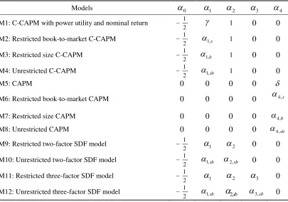
Table 1 provides a summary of restrictions for each asset pricing models

implied by its no-arbitrage condition. C-CAPM with power utility and nominal

returns (M1) implies that the CRRA is constant and should be the same across the

cross-section of expected returns for no arbitrage opportunities in the market. M1 is

the restricted version of C-CAPM. On the other hand, allowing the coefficients on the

conditional covariances of returns with consumption to be different generates an

unrestricted version of C-CAPM (M4). The double-sorted, 25 size and

book-to-market equity ratio portfolios generate two more versions of C-CAPM with power

utility: restricted book-to-market model (M2) and restricted size model (M3). M2

allows portfolios with different size groups to have different coefficients on the

consumption covariances, while M3 allows the coefficients for portfolios with

different book-to-market-equity ratio groups to be different. Similarly, these

restrictions of C-CAPM are applied to the CAPM, where the market price of risk is

expected to be the same across assets, (M5-M8). In addition, the restricted and

unrestricted general SDF models, based on two (consumption growth and inflation)

and three macroeconomic variables (consumption growth, inflation and industrial

production growth), are given by M9-M12. In sum, all the above asset pricing models

can be represented as restricted versions of the SDF model,

1 0, 1 1, 1 1 2, 1 1

( sb f) ( sb) ( , sb) ( , sb)

t t t sb t t sb t t t sb t t t

E i_ i  V i_  Cov c_ i_  Cov _ i_

3, ( 1, 1) 4, ( 1, 1)

sb m sb

sbCovt qt it sbCov it t it

 _{ }  _{ }

   (7)

where s and b indicate size and book-to-market ratio groups that the characteristics

portfolios belong to, respectively, and q_t is industrial production. The different asset

Table 1

Restrictions on the No-arbitrage Condition

sandbindicate size and book-to-market groups for the characteristics portfolios. The numbers are in ascending order of magnitude. The smallest size is denoted bys= 1 while the lowest book-to-market ratio is represented by b = 1.  denotes constant coefficient of relative risk aversion (CRRA)._i represents a coefficient for each conditional covariance in Equation 8.

Models ₀ ₁ ₂ ₃ ₄

M1: C-CAPM with power utility and nominal return 1

2

  1 0 0

M2: Restricted book-to-market C-CAPM 1

2

 _1,s 1 0 0

M3: Restricted size C-CAPM 1

2

 _1,b 1 0 0

M4: Unrestricted C-CAPM 1

2

 _1,sb 1 0 0

M5: CAPM 0 0 0 0 

M6: Restricted book-to-market CAPM 0 0 0 0 4,s

M7: Restricted size CAPM 0 0 0 0 4,b

M8: Unrestricted CAPM 0 0 0 0 4,sb

M9: Restricted two-factor SDF model 1

2

 ₁ ₂ 0 0

M10: Unrestricted two-factor SDF model 1

2

 _1,sb _2,sb 0 0

M11: Restricted three-factor SDF model 1

2

 ₁ ₂ ₃ 0

M12: Unrestricted three-factor SDF model 1

2

4. Econometric Framework

We follow the same econometric approach here as in Smith and Wickens (2002), and

Smith, Sorensen, and Wickens (2008, 2010), and Abhakorn, Smith, and Wickens

(2013) by using the multivariate generalized autoregressive conditional

heteroskedasticity in mean model (MGM) to estimate the joint distribution of the

excess return on equity with macroeconomic factors in such a way that the return

satisfies the no-arbitrage condition under the SDF framework. This approach is

achieved by including conditional covariances of the excess equity returns and the

macroeconomic factors in the mean of the asset pricing equations and constraining the

coefficients on these time-varying, conditional covariances according to the

no-arbitrage condition implied by each asset-pricing model.

Let x_{t 1} (r_{1, 1t} r_tf,...,r_{i t, 1} r_tf,c_t1,_t1,q_t1) ' which contains n variables and i

returns, as several portfolios are estimated at the same time. This specification is an

extension of the MGM in Smith and Wickens (2002). Consumption, inflation, and

industrial productions are included, as they give rise to the discount factors in the SDF

model, M1-M12 in Table 1, through their conditional covariances with the excess

returns. Additional macroeconomic variables can be included in this vector if they

improve the estimate of the joint distribution. The MGM model can then be written as

t +1 t t +1 t +1

x = + x + g + ,

where

|I_t ~ N(0, )

t+1 Ht+1 ,

( )

vech 

t+1 t+1

g H .

where, is a n1 vector of constant, is a nn matrix of coefficients in the

vector autoregressive (VAR) part (included to obtain better representation of the error

terms), is a nn matrix of coefficients of in-mean component, _t+1 is an n1

vector of errors, and i number of equity returns. The vech operator converts the

lower triangle of a symmetric matrix into a vector. The error term, _t+1 , is

conditionally normally distributed with mean zero and with conditional covariance

matrix H_t+1. The first i rows of the model is restricted to satisfy the no-arbitrage

condition as follows: 1) the first i rows of must be zero; 2) the first i rows of

i+1 to i+3 rows of are all zero; and 4) the first i elements of is zero. A

likelihood ratio test is used to provide test statistics for the restrictions implied by the

no-arbitrage condition in M1-M12 as given in Table 1.

While the MGM model is convenient, it is heavily parameterized, which can create

numerical problems in finding the maximum of the likelihood function due to the

likelihood of being relatively flat, and hence uninformative. Therefore, to complete

the model parameterization for the conditional covariance matrix H_t+1 with the view

toward restricting the number of coefficients being estimated, the specification of the

conditional covariance matrix is chosen to be the vector diagonal model with variance

targeting (Ding and Engle, 2001), which can be written as follows,

/

( ) ( )

 / / /  / / 

t+1 0 t t t

H H ii - aa - bb aa  bb H

where  denotes Hadamard product, H₀ is the observed sample covariance matrix,

and a and b are n1 vectors. The number of parameters to be estimated reduces to

2n. This model is particularly attractive when we estimate several excess returns

simultaneously, each with its own arbitrage condition. In addition, the zero

restrictions on the coefficients for excess returns in the VAR part of the

macroeconomic variables are imposed to further reduce the number of parameters in

the MGM model. Estimating the restricted and unrestricted C-CAPM (M1 and M4)

for the 25 portfolios sorted by size and book-to-market ratio involve 69 and 93

parameters, respectively, while for the CAPM (M5 and M8) involving 53 and 78

parameters; we need to include only the market return, instead of the macroeconomic

factors, in the joint distribution. We are unable to estimate M10 and M12 for the 25

portfolios, as doing so involves estimating too many parameters for our sample size

(118 and 143 parameters, respectively); hence we include the two data sets of the 10

portfolios formed for size and book-to-market ratio separately to test for these general

two- and three-factor SDF models, in addition to using these one-sorted portfolios to

5. Estimation Results

5.1 Data

The data are monthly from 1960.2 to 2004.11 for the U.S. (538 observations). The

return on the market portfolio is the value-weighted return on all stocks. The return on

a risk-free asset is the one-month Treasury bill rate. Table 2 shows the summary

statistics for the 25 value-weighted portfolios, which are the intersections of 5

portfolios formed on size and 5 portfolios formed on the ratio of book-to-market ratio.

There are also two sets of ten portfolios sorted by size and book-to-market ratio

separately (Table 3). All of the return variables are obtained from Kenneth French’s

websiteb. Real non-durable growth consumption is from the Federal Reserve Bank of

St. Louis. CPI inflation and the volume index of industrial production are both from

Datastream.

b

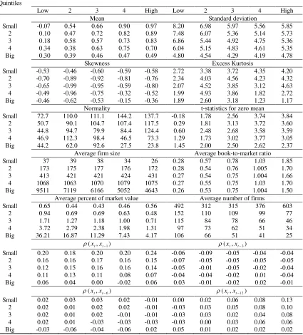
Table 2

SummaryStatistics: 25 Size and Book-to-Market Portfolios

The table presents descriptive statistics for the excess returns on the 25 portfolios formed as the intersections of the five size and book-to-market ratio groups. Data and full definition of the returns can be found on Kenneth French’s webpage. The returns are monthly value-weighted from 1960.2 to 2004.11, 538 observations. t-stat is the test statistics for zero mean hypothesis.(xt, xt-i) represents the autocorrelation coefficients over the time intervalimonth (s).

Size Quintiles

Book-to-Market Equity Quintiles

Low 2 3 4 High Low 2 3 4 High

Mean Standard deviation

Small -0.07 0.54 0.66 0.90 0.97 8.20 6.98 5.97 5.56 5.85 2 0.10 0.47 0.72 0.82 0.89 7.48 6.07 5.36 5.14 5.73 3 0.18 0.58 0.57 0.73 0.83 6.86 5.44 4.92 4.75 5.36 4 0.34 0.38 0.63 0.75 0.70 6.04 5.15 4.83 4.61 5.35 Big 0.30 0.39 0.46 0.47 0.49 4.80 4.54 4.29 4.19 4.78

Skewness Excess Kurtosis

Small -0.53 -0.46 -0.60 -0.59 -0.58 2.72 3.38 3.72 4.35 4.20 2 -0.70 -0.89 -0.92 -0.81 -0.76 2.34 4.03 4.56 4.23 4.32 3 -0.65 -0.99 -0.95 -0.59 -0.80 2.07 4.52 3.85 3.12 4.63 4 -0.49 -0.96 -0.75 -0.32 -0.52 1.99 4.93 3.86 1.82 2.72 Big -0.46 -0.62 -0.53 -0.15 -0.36 1.89 2.60 3.18 1.23 1.17

Normality t-statistics for zero mean

Small 72.7 110.0 111.1 144.2 137.7 -0.18 1.78 2.56 3.74 3.84 2 50.7 90.1 104.7 107.4 117.5 0.29 1.81 3.13 3.72 3.60 3 44.8 94.7 79.9 84.4 124.4 0.60 2.48 2.68 3.58 3.59 4 46.9 112.3 98.4 46.5 73.3 1.29 1.73 3.02 3.77 3.05 Big 44.2 62.0 92.6 27.5 23.8 1.45 2.00 2.50 2.62 2.37

Average firm size Average book-to-market ratio Small 37 39 38 34 26 0.28 0.57 0.78 1.03 1.85

2 173 175 177 176 172 0.28 0.54 0.76 1.005 1.70 3 413 421 421 424 431 0.27 0.54 0.75 1.004 1.66 4 1068 1063 1070 1079 1075 0.27 0.55 0.75 1.03 1.70 Big 9511 7119 6166 5052 4643 0.26 0.53 0.75 1.004 1.50

Average percent of market value Average number of firms

Small 0.65 0.44 0.43 0.46 0.56 492 312 315 376 603 2 0.94 0.69 0.69 0.63 0.48 152 110 109 99 77 3 1.71 1.27 1.18 1.00 0.71 115 84 78 66 46 4 3.72 2.79 2.38 1.98 1.31 97 73 62 51 34 Big 36.21 16.87 11.29 7.43 4.17 106 66 51 41 25

1

(x xt, t )

  (x xt, t3)

Small 0.20 0.18 0.20 0.20 0.24 -0.06 -0.09 -0.05 -0.04 -0.04 2 0.16 0.16 0.17 0.16 0.15 -0.07 -0.05 -0.05 -0.05 -0.05 3 0.12 0.15 0.16 0.16 0.14 -0.05 -0.01 -0.05 -0.02 -0.04 4 0.11 0.13 0.11 0.08 0.07 -0.04 -0.04 -0.02 0.01 -0.04 Big 0.06 0.04 0.00 -0.02 0.06 0.03 -0.01 -0.02 0.02 -0.01

6

(x xt, t )

  (x xt, t12)

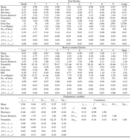
Table 3

Summary Statistics: 10 Industry Portfolios and Explanatory Variables

The table presents descriptive statistics for the returns on the 10 portfolios and explanatory variables. The returns are monthly value-weighted from 1960.2 to 2004.11, 538 observations. Data and full definition of the 10 portfolios can be found on Kenneth French’s webpage.im,t+1anditfare the returns on the market portfolios and one-month Treasury bill rate respectively. Consumption growth, inflation, and industrial production growth are represented byct+1,t+1, andqt+1respectively. Std. Dev is the standard deviation. t-stat is the t-statistic for zero mean hypothesis. t-stat is the test statistics for zero mean hypothesis.  ( xt , xt-i ) represents the autocorrelation coefficients over the time interval i month(s). BM denotes book-to-market equity ratio. Firm size, book-to-market equity ratio, percent of the market, and number of firms are in average terms.

Size Deciles

Small 2 3 4 5 6 7 8 9 Large

Mean 1.04 0.98 1.03 0.98 1.01 0.92 0.98 0.95 0.91 0.79

Std. Dev. 6.32 6.26 5.99 5.80 5.55 5.25 5.11 4.98 4.54 4.26

Skewness -0.53 -0.64 -0.78 -0.86 -0.85 -0.84 -0.71 -0.64 -0.56 -0.52

Excess Kurtosis 3.23 3.52 3.22 3.56 3.42 3.20 3.33 2.49 2.45 2.13

Normality 94.89 96.69 72.24 77.02 73.66 68.42 81.48 56.85 52.81 50.40

t-stat 3.81 3.64 3.98 3.91 4.23 4.08 4.45 4.41 4.64 4.29

Firm Size 21 78 139 219 338 512 803 1346 2597 12780

% of Market 1.47 1.37 1.62 2.00 2.59 3.33 4.69 7.39 13.23 62.31

No. of firms 2123 523 347 272 229 194 175 164 152 146

1

(x x_t, _t )

  0.24 0.17 0.16 0.16 0.14 0.01 0.12 0.09 0.08 0.01

3

(x x_t, _t )

  -0.05 -0.07 -0.07 -0.06 -0.05 -0.04 -0.03 -0.04 -0.03 0.03

6

(x x_t, _t )

  0.01 0.02 0.01 0.02 0.02 0.01 0.00 0.00 -0.02 -0.03

12

(x xt, t )

  0.08 0.04 0.03 0.03 0.01 0.01 0.01 0.01 0.01 0.05

Book-to-market Deciles

Low 2 3 4 5 6 7 8 9 High

Mean 0.67 0.85 0.87 0.86 0.93 0.99 1.05 1.09 1.12 1.21

Std. Dev. 5.24 4.77 4.73 4.66 4.35 4.36 4.26 4.26 4.64 5.33

Skewness -0.42 -0.69 -0.81 -0.66 -0.70 -0.67 -0.17 -0.28 -0.41 -0.37

Excess Kurtosis 1.67 2.76 3.88 3.12 4.24 3.54 1.80 2.11 2.11 3.26

Normality 38.09 63.18 92.12 78.47 121.46 93.76 50.24 60.74 54.66 112.13

t-stat 2.91 4.14 4.28 4.28 4.96 5.27 5.71 5.93 5.59 5.25

Firm Size 1582 1178 981 813 723 576 527 433 349 177

BM 0.20 0.37 0.49 0.60 0.71 0.82 0.94 1.10 1.35 2.03

% of Market 32.80 15.27 11.46 8.88 7.79 6.20 5.76 4.88 4.29 2.68

No. of firms 592 370 333 312 308 307 312 322 351 433

1

(x x_t, _t )

  0.09 0.07 0.07 0.08 0.05 0.03 0.04 0.05 0.09 0.12

3

(x xt, t )

  0.02 -0.01 -0.02 -0.03 -0.04 0.01 0.02 -0.01 -0.03 -0.03

6

(x x_t, _t )

  -0.02 -0.01 -0.04 -0.04 -0.03 0.00 -0.06 -0.03 -0.02 -0.02

12

(x x_t, _t )

  0.02 0.02 0.01 0.01 0.02 0.02 0.01 0.07 0.06 0.07

Explanatory variables

, 1

m t

i  itf ct1 t1 qt1 Correlation

Mean 0.94 0.46 0.23 0.35 0.25 im t,1 itf ct1 t1 qt1

Std. Dev. 4.41 0.23 0.73 0.30 0.75 itf -0.04 1.00

Skewness -0.46 1.041 -0.04 0.99 -0.62 ct1 0.15 -0.09 1.00

Excess Kurtosis 1.90 1.70 1.37 1.68 2.98 t1 -0.14 0.54 -0.20 1.00

Normality 44.85 98.95 33.56 82.25 75.70 qt1 -0.03 -0.16 0.14 -0.10 1.00

1

(x x_t, _t )

  0.06 0.95 -0.36 0.64 0.36

3

(x x_t, _t )

  0.00 0.90 0.14 0.53 0.27

6

(x x_t, _t )

  -0.02 0.84 0.01 0.52 0.09

12

(x x_t, _t )

The descriptive statistics for the excess returns for the 25 portfolios in Table 2 are

similar to those in Fama and French (1993 and 2006) for the periods 1963-1991 and

1963-2004 respectively, thus indicating the value effect and relatively weak size

effect. This relatively weak size effect is also seen in Table 3 where one-characteristic

sorted portfolios are considered. In general, all excess returns and macroeconomic

variables appear to have negative skewness, excess kurtosis, and non-normality,

except for the risk-free rate and inflation, which display positive skewness and show

persistent volatility.

5.2 Estimates

5.2.1 C-CAPM

A full set of model estimates with their restricted versions for C-CAPM with power

utility and nominal returns is reported in Table 4. A likelihood ratio test is used to

examine the hypothesis implied by each restricted model against the unrestricted

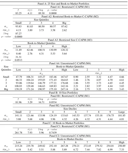
model, M4. For M1, the conditional covariance of returns with consumption is highly

significant, but the size of the coefficient, 83.25, implies an implausibly large CRRA,

which is a common feature of consumption-based models (Campbell, 2002,

Cochrane, 2008, Yogo (2006), Smith, Sorensen, and Wickens, 2008, 2010) except for

C-CAPM with garbage growth of Savov (2011).

For M2, all five consumption coefficients are significant, and the likelihood ratio

rejects the hypothesis that portfolios within different book-to-market equity ratio

quintiles have the same coefficient at any conventional levels. The test statistic for the

restrictions against the unrestricted model M4 is close to that for M1, implying that

the differences in the coefficients across size have little weight on the behavior of the

estimated returns. On the other hand, the likelihood ratio test marginally fails to reject

M3 (pvalue0.0513); restricting the consumption coefficients for portfolios within

the same size quintiles to be the same does not exclude significant information about

the excess returns. In other words, size has no, or a relatively weak, relation to the

consumption coefficient. In fact, the coefficients in M2 for each size quintile look

very similar, while those in M3 for each book-to-market equity ratio quintiles increase

consumption covariance coefficient for the lowest book-to-market equity ratio

quintiles in M3 is not significantly different from zero.

M4 has 23 coefficients that are significant at conventional significance levels. All

coefficients range widely from 47.79 to 247.14. Looking down each column, there is

no clear pattern in the values of the coefficients across the size quintiles, whilst when

looking across each row; the coefficients tend to rise as the book-to-market ratio

increases. Like the insignificance of the consumption coefficient on the lowest

book-to-market quintile in M3, the remaining 2 coefficients for the lowest book-book-to-market

quintile and the first 2 smallest size quintiles are not significantly different from zero.

The insignificance of the coefficients for the lowest book-to-market quintiles of the 25

portfolios is consistent with the evidence from other empirical asset pricing studies on

the 25 portfolios (Fama and French, 2008, Lettau and Lugvigson, 2001, Parker and

Julliard, 2005, Yogo, 2006, and Savov, 2011) where the pricing models they propose

also have difficulty explaining the portfolios in the smallest size and lowest

book-to-market quintiles (small growth portfolio). This inability may be due to limits to

arbitrage from short-sale constraints for these portfolios, and thus frictionless

equilibrium models, including C-CAPM, cannot explain the returns on these small

growth portfolios (Yogo, 2006).

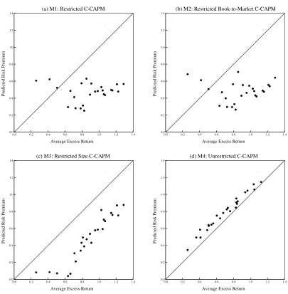
Figure 1 shows a scatter plot of average actual and estimated excess returns in M1

to M4 for the 25 portfolios. If the pricing model fits the data well, the points should

all lie on a 45-degree line. In Figure 1(d), M4 appears to best explain the excess return

on these portfolios and is more or less as good as the modified versions of C-CAPM

and the Fama and French three-factor model. The differences in the estimated risk

premium and actual excess return ranges from 0.01% to 0.18% per month, which is

lower than those in M1-M4.

Figures 1(a) and 1(b) show that the estimated risk premia from M1 and M2 are

similar, implying that imposing the restrictions on size quintiles does not affect the

behavior of risk premia. On the other hand, allowing the consumption coefficients to

be different, as in M3, improves the performance of the model sharply, except for the

that book-to-market equity ratio seems to have additional information about the

average excess returns that is not captured by C-CAPM.

Table 4

Estimates of C-CAPM

The table presents the estimates of the C-CAPM (M1-M4): 1960.2-2004.11, 538 observations. 

denotes the coefficient relative risk aversion and _i represents a coefficient for each conditional covariance in Equation 8. ( )t  andt( )i are their corresponding t–statistics respectively. The pricing

models (M1-M4) are tested against each other using the log-likelihood ratio test. 2log represents the likelihood ratio statistic. The corresponding p-value at 5% significance level is denoted byp-value.

Panel A: 25 Size and Book-to-Market Portfolios Panel A1: Restricted C-CAPM (M1)  t( ) 2 lo g pva lu e

83.25 4.11 89.30 0.0000

Panel A2: Restricted Book-to-Market C-CAPM (M2) Size Quintiles

Small 2 3 4 Big

1s

 93.83 81.83 80.50 80.57 87.62

1

( _s)

t 4.13 3.89 3.73 3.58 2.62

2 lo g 87.27

pva lu e 0.0000

Panel A3: Restricted Size C-CAPM (M3) Book-to-Market Quintiles

Low 2 3 4 High

1b

 11.49 62.46 100.51 130.99 128.32

1

( _b)

t  0.40 2.76 4.31 5.53 5.64

2 lo g 31.31

pva lu e 0.0513

Panel A4: Unrestricted C-CAPM (M4) Size

Quintiles

Book-to-Market Quintiles

Low 2 3 4 High Low 2 3 4 High

sb

 t(_sb)

Small 47.79 106.31 145.27 183.46 167.67 0.90 2.55 3.32 4.47 4.66 2 66.32 104.24 155.03 171.43 164.63 1.46 2.76 4.07 4.70 4.61 3 93.06 119.64 146.79 177.21 176.68 1.86 3.55 3.73 4.65 4.45 4 108.03 129.48 146.63 169.83 142.16 2.21 2.82 3.97 4.44 3.83 Big 139.19 171.24 190.97 175.10 247.14 2.16 2.75 3.22 3.35 3.43

Panel B: 10 Size Portfolios

Panel B1: Restricted C-CAPM (M1)  t( ) 2 lo g pva lu e

81.96 3.29 16.71 0.0534

Panel B2: Unrestricted C-CAPM (M4) Size Deciles

Small 2 3 4 5 6 7 8 9 Large

1s

 141.11 121.66 133.98 124.19 133.63 143.53 137.74 153.18 176.75 181.85

1

( _s)

t 3.88 3.68 4.06 3.96 4.32 4.26 4.32 4.31 4.44 4.01 Panel C: 10 Book-to-Market Portfolios

Panel C1: Restricted C-CAPM (M1)  t( ) 2 lo g pva lu e

261.78 7.93 5.96 0.7439

Panel C2: Unrestricted C-CAPM (M4) Book-to-Market Deciles

Low 2 3 4 5 6 7 8 9 High

1b

 215.24 235.78 249.82 252.10 267.28 270.21 272.45 279.32 254.01 250.89

1

( _b)

Figure 1

Cross-Sectional Fit: C-CAPM for the 25 Size and Book-to-Market Portfolios The figure plots average actual versus predicted excess returns (% per month) for the 25 size and book-to-market portfolios. The estimated models are (a) M1, (b) M2, and (c) M3, and (d) M4. The average excess returns are adjusted for the Jensen effect.

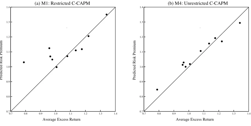
We estimate M1 and M4 for the two one-characteristic sorted portfolios to

investigate whether these provide similar information to the double-sorted portfolios.

Panels B and C in Table 4 show that C-CAPM with power utility performs better, as

neither of the M1 is rejected, suggesting that sorting stocks according to size and

book-to-market ratio may more accurately distinguish stocks. For the 10 size

portfolios, all coefficients on the consumption covariances in M4 are significant, and

the model fits the data better than M1 (Figure 2). This is also true for the 10

book-to-market ratio portfolios (Figure 3). In addition, the consumption coefficient for the

portfolio in the lowest book-to-market quintile is highly significant, while those for 0.0 0.2 0.4 0.6 0.8 1.0 1.2 1.4

0.0 0.2 0.4 0.6 0.8 1.0 1.2 1.4 P re d ic te d R is k P re m iu m

Average Excess Return

(a) M1: Restricted C-CAPM

0.0 0.2 0.4 0.6 0.8 1.0 1.2 1.4 0.0 0.2 0.4 0.6 0.8 1.0 1.2 1.4 P re d ic te d R is k P re m iu m

Average Excess Return

(b) M2: Restricted Book-to-Market C-CAPM

0.0 0.2 0.4 0.6 0.8 1.0 1.2 1.4 0.0 0.2 0.4 0.6 0.8 1.0 1.2 1.4 P re d ic te d R is k P re m iu m

Average Excess Return

(c) M3: Restricted Size C-CAPM

0.0 0.2 0.4 0.6 0.8 1.0 1.2 1.4 0.0 0.2 0.4 0.6 0.8 1.0 1.2 1.4 P re d ic te d R is k P re m iu m

Average Excess Return

the small growth portfolios in the 25 portfolios are not. The descriptive statistics in

Table 2 show that the average book-to-market ratios for these two portfolios are

similar, while their average firm sizes are very different. Firms in the smallest size

and the lowest book-to-market quintiles seem to be much smaller than other firms in

the lowest book-to-market quintiles. Therefore, additional information that is not

captured by C-CAPM may be associated with both book-to-market equity ratio as

well as size. One possible explanation is that this extra dimension of risk arises from

the investment growth prospect of firms. Abhakorn, Smith, and Wickens (2013) find

that, in the C-CAPM framework, the mimicking return factor related to

book-to-market ratio (HML) can explain the 25 Fama-French portfolios across size quintiles as

well as across book-to-market ratio quintiles. In this regard, they assert that HML may

represent risk associated with the investment growth prospects of firm as low

book-to-market ratio firms may be expected to have higher rates of growth while small firms

may also be expected to behave similarly. This interpretation of the extra dimension

of risk is also consistent with Brennan, Wang, and Xia (2004) and Li, Vassalou, and

Xing (2006). These two studies propose asset pricing models based on investment

related factors that can explain the cross-section of equity returns well.

Figure 2

Cross-Sectional Fit: C-CAPM for the 10 Size Portfolios

The figure plots average actual versus predicted excess returns (% per month) for the 10 size portfolios. The estimated models are (a) M1 and (b) M4. The average excess returns are adjusted for the Jensen effect.

0.2 0.4 0.6 0.8 1.0 1.2

0.2 0.4 0.6 0.8 1.0 1.2

P

re

d

ic

te

d

R

is

k

P

re

m

iu

m

Average Excess Return

(a) M1: Restricted C-CAPM

0.2 0.4 0.6 0.8 1.0 1.2

0.2 0.4 0.6 0.8 1.0 1.2

P

re

d

ic

te

d

R

is

k

P

re

m

iu

m

Average Excess Return

Figure 3

Cross-Sectional Fit: C-CAPM for the 10 Book-to-Market Ratio Portfolios The figure plots average actual versus predicted excess returns (% per month) for the 10 book-to-market ratio portfolios. The estimated models are (a) M1 and (b) M4. The average excess returns are adjusted for the Jensen effect.

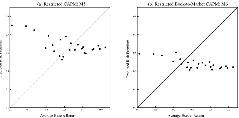
5.2.2 CAPM

Table 5 reports the estimation results for all versions of CAPM. The market price of

risk in M5 is 2.77 with a t-statistics of 2.94 and is lower than those reported in earlier

related studies for the U.S. market (Harvey (1989) and Ng (1991)). Comparing M6 to

M2, where the coefficients for the first three size quintiles are relatively less

significant, suggests that CAPM cannot price relatively small portfolios well and that

there is more information in these portfolio returns related to size left unexplained by

CAPM than by C-CAPM discussed above. This inability to price small portfolios has

nothing to do with the book-to-market ratio. Moreover, as in M3, the coefficient on

the market return for the portfolios in the lowest book-to-market ratio in M7 is not

significant.

0.7 0.8 0.9 1.0 1.1 1.2 1.3 1.4 0.7

0.8 0.9 1.0 1.1 1.2 1.3 1.4

P

re

d

ic

te

d

R

is

k

P

re

m

iu

m

Average Excess Return

(a) M1: Restricted C-CAPM

0.7 0.8 0.9 1.0 1.1 1.2 1.3 1.4 0.7

0.8 0.9 1.0 1.1 1.2 1.3 1.4

P

re

d

ic

te

d

R

is

k

P

re

m

iu

m

Average Excess Return

Table 5

Estimates of the CAPM

The table presents the estimates of the CAPM (M5-M8): 1960.2-2004.11, 538 observations. denotes the market price of risk and_i represents a coefficient for each conditional covariance in Equation 8.

( )

t andt( )_i are their corresponding t–statistics respectively. The pricing models (M5-M8) are tested against each other using the log-likelihood ratio test. 2log represents the likelihood ratio statistic. The corresponding p-value at 5% significance level is denoted byp-value.

Panel A: 25 Size and Book-to-Market Portfolios

Panel A1: Restricted CAPM (M5)  t( ) 2 lo g pva lu e

2.77 2.94 153.72 0.0000

Panel A2: Restricted Book-to-Market CAPM (M6) Size Quintiles

Small 2 3 4 Big

4s

 1.70 1.69 1.74 2.03 2.61

4

( s)

t  1.56 1.68 1.80 2.11 2.79

2 lo g 110.22

pva lu e 0.0000

Panel A3: Restricted Size CAPM (M7) Book-to-Market Quintiles

Low 2 3 4 High

4b

 0.93 2.54 3.51 4.57 4.73

4

( _b)

t  0.93 2.68 3.75 4.79 4.89

2 lo g 43.04

pva lu e 0.0020

Panel A4: Unrestricted CAPM (M8) Size

Quintiles

Book-to-Market Quintiles

Low 2 3 4 High Low 2 3 4 High

4sb

 t(4sb)

Small 0.02 2.20 3.02 4.37 4.51 0.02 1.75 2.59 3.78 3.93 2 0.76 2.30 3.55 4.36 4.34 0.67 2.16 3.40 4.10 4.02 3 1.30 3.05 3.14 4.37 4.26 1.15 3.00 3.14 4.26 3.92 4 1.94 2.26 3.59 4.16 3.57 1.74 2.26 3.53 4.04 3.27 Big 1.93 2.22 2.70 3.20 3.21 1.81 2.15 2.53 2.91 2.63

Panel B: 10 Size Portfolios

Panel B1: Restricted CAPM (M5)  t( ) 2 lo g pva lu e

-0.47 -0.34 811.30 0.0000

Panel B2: Unrestricted CAPM (M8) Size deciles

Small 2 3 4 5 6 7 8 9 Large

4s

 3.57 3.07 3.41 3.13 3.44 3.27 3.29 3.26 3.23 2.45

4

( _s)

t  3.46 3.27 3.74 3.44 3.93 3.69 3.82 3.80 3.77 2.88 Panel C: 10 Book-to-market Portfolios

Panel C1: Restricted CAPM (M5)  t( ) 2 lo g pva lu e

1.98 1.79 404.85 0.0000

Panel C2: Unrestricted CAPM (M8) Book-to-market Deciles

Low 2 3 4 5 6 7 8 9 High

4b

 3.14 4.29 4.68 4.76 5.50 5.73 6.64 6.96 6.18 6.24

4

( _b)

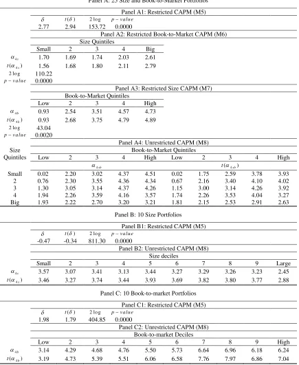
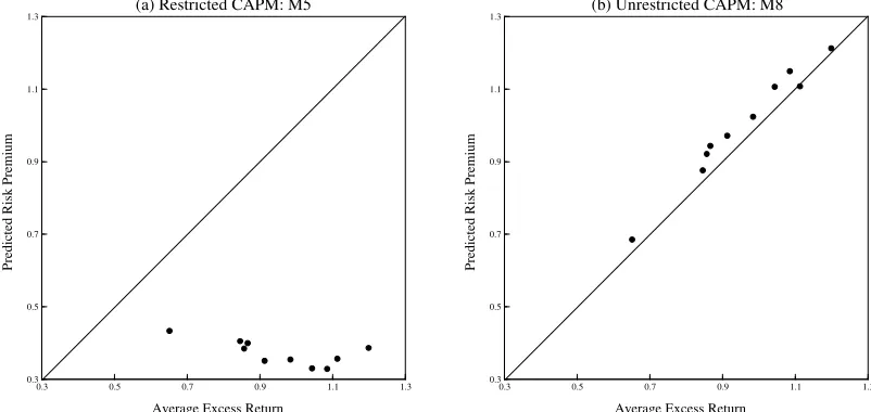
M5, M6, and M7 are rejected relative to the unrestricted model M8 based on their

likelihood ratio statistics of 153.72, 110.22, and 43.04 respectively. The likelihood

ratio statistics for CAPM are all larger than those for C-CAPM. As in C-CAPM,

allowing the coefficients on conditional covariances of market return with individual

excess return to be different offers extra information about the cross-section of the

equity returns. As can be seen from Figure 4, M8 can explain the variation in the cross

section well while M5 is not able to explain both size and value effects as in previous

studies (e.g. Fama and French , 1992 and 2006 and Lewellen and Nagel, 2006).

In M8, 20 coefficients on conditional covariances of returns with the market return,

including one for the market return (the coefficient on the variance), are more than 2

standard errors different from zero, while the other 3 coefficients are significant at the

10% significance level. The coefficients for the first 3 size and lowest book-to-market

quintiles are insignificant at any conventional level. These coefficients range from

0.02 to 4.51, exhibiting a clear positive relation with book-to-market ratio. However,

any relation between the coefficients and size can be seen only from the portfolios in

the last two book-to-market quintiles.

Figure 4

Cross-Sectional Fit: CAPM for the 25 Size and Book-to-Market Portfolios The figure plots average actual versus predicted excess returns (% per month) for the 25 size and book-to-market portfolios. The estimated models are (a) M5, (b) M6, and (c) M7, and (d) M8. The average excess returns are adjusted for the Jensen effect.

-0.1 0.1 0.3 0.5 0.7 0.9

-0.1 0.1 0.3 0.5 0.7 0.9

P

re

d

ic

te

d

R

is

k

P

re

m

iu

m

Average Excess Return

(a) Restricted CAPM: M5

-0.1 0.1 0.3 0.5 0.7 0.9

-0.1 0.1 0.3 0.5 0.7 0.9

P

re

d

ic

te

d

R

is

k

P

re

m

iu

m

Average Excess Return

M5 for the two sets of 10 portfolios does not perform well since the market

price of risk is of relatively low significance and in the case of the 10 size portfolios,

the market price of risk has the wrong sign. Therefore, the likelihood ratio test rejects

M5 for both 10 portfolios. M8 fits the data better than M5 (Figures 5 and 6), but its

coefficients exhibit a negative relation with size and a negative relation with

book-to-market ratio for both 10 portfolios as in the case of the 25 portfolios. On the other

hand, the relation between the consumption coefficients and firm characteristics in

C-CAPM can be seen only in the case of the 25 portfolios. Thus, C-C-CAPM can explain

size effect, but it has difficulty explaining the value effects; this exposure to the value

premium appears to be associated with both the book-to-market ratio and, to some

extent, with size.

-0.1 0.1 0.3 0.5 0.7 0.9

-0.1 0.1 0.3 0.5 0.7 0.9

P

re

d

ic

te

d

R

is

k

P

re

m

iu

m

Average Excess Return

(c) Restricted Size CAPM: M7

-0.1 0.1 0.3 0.5 0.7 0.9

-0.1 0.1 0.3 0.5 0.7 0.9

P

re

d

ic

te

d

R

is

k

P

re

m

iu

m

Average Excess Return

Figure 5

Cross-Sectional Fit: CAPM for the 10 Size Portfolios

The figure plots average actual versus predicted excess returns (% per month) for the 10 size portfolios. The estimated models are (a) M5 and (b) M8. The average excess returns are adjusted for the Jensen effect.

Figure 6

Cross-Sectional Fit: CAPM for the 10 Book-to-Market Portfolios

The figure plots average actual versus predicted excess returns (% per month) for the 10 book-to-market ratio portfolios. The estimated models are (a) M5 and (b) M8. The average excess returns are adjusted for the Jensen effect.

5.2.3 C-CAPM and CAPM

We further investigate the ability of C-CAPM (M1) and CAPM (M4) by comparing

the behavior of the conditional covariances in both models, as given in Table 6 below,

with the average excess returns of the 25 portfolios shown in Table 2. The -0.2 0.0 0.2 0.4 0.6 0.8 1.0

-0.2 0.0 0.2 0.4 0.6 0.8 1.0 P re d ic te d R is k P re m iu m

Average Excess Return

(a) Restricted CAPM: M5

-0.2 0.0 0.2 0.4 0.6 0.8 1.0 -0.2 0.0 0.2 0.4 0.6 0.8 1.0 P re d ic te d R is k P re m iu m

Average Excess Return

(b) Unrestricted CAPM: M8

0.3 0.5 0.7 0.9 1.1 1.3

0.3 0.5 0.7 0.9 1.1 1.3 P re d ic te d R is k P re m iu m

Average Excess Return

(a) Restricted CAPM: M5

0.3 0.5 0.7 0.9 1.1 1.3

0.3 0.5 0.7 0.9 1.1 1.3 P re d ic te d R is k P re m iu m

Average Excess Return

consumption covariance obtained from the estimation of C-CAPM decreases, as we

move down the column, indicating a negative relation with size. Thus, C-CAPM can

capture the size effect. However, in the lowest book-to-market quintiles, average

excess returns increase as the size of the portfolios grows larger. This result is

consistent with the results in Table 4 where the coefficients for these portfolios in M3

and M4 are not significant from zero.

Table 6

Conditional Covariances of the Returns on the 25 Portfolios in M1 and M5 The table shows the average conditional covariances of the returns with consumption and market returns as implied by the C-CAPM and CAPM, respectively. Each conditional covariance is given in percent per month and estimated by the multivariate GARCH in the mean.

Book-to-market ratio Quintile Size

Quintile Low 2 3 4 High

Panel A: Conditional covariance of consumption

Small 0.32218 0.28800 0.31130 0.22016 0.27699

2 0.24066 0.23827 0.23237 0.17594 0.20899

3 0.19671 0.17586 0.16247 0.15597 0.17918

4 -0.00131 -0.00166 -0.00138 0.00593 0.00496

Big 0.00304 0.00001 -0.00133 -0.00127 -0.00040

Panel B: Conditional covariance of market return

Small 0.32143 0.35714 0.25829 0.25272 0.28785

2 0.24282 0.22963 0.21088 0.24303 0.17777

3 0.23056 0.18894 0.18875 0.17934 0.16103

4 0.18551 0.21742 0.20223 0.15693 0.20226

Big 0.27074 0.24804 0.19669 0.16809 0.16478

C-CAPM appears to miss the value premium completely by not producing

dispersion in the consumption covariance across the book-to-market quintiles. In fact,

the consumption covariances for the 5 portfolios in the highest book-to-market

quintile seem to be slightly lower than those in the lowest book-to-market quintiles,

indicating lower risk premium is implied by C-CAPM. On the other hand, the

condition covariances of the returns with the market returns in CAPM, in addition to

having a similar behavior across book-to-market quintiles as consumption covariances,

appear not to be able to capture the size effect as well. The dispersion of the market

covariances is not big enough to explain the differences in the excess returns across

size, confirming our previous results where the coefficients for the first two size

We add a constant term in M1-M8 for the estimation of the 25 portfolios to

measure variation in excess returns that was left unexplained in each model. In

general, we expect the constant term in C-CAPM to be of more significance than in

those in CAPM because pricing asset returns with market return is expected to be

more precise than using aggregate consumption data. However, Table 7 shows that for

the magnitude of the constant terms in CAPM, 1.98 is larger than that for C-CAPM at

0.86. This larger magnitude of CAPM is present in every restricted version. The

magnitude of the constant is also larger than in Fama and French (1993) with a

constant for the CAPM being 0.04 to 0.57 (in absolute terms).

Table 7 Constant term

The table presents the estimates for the constant term, in all versions of the C-CAPM and CAPM, M1-M8 in Table 1, for the 25 portfolios formed based on size and book-to-market ratio. The number in the parentless is the t-statistic associated with each constant term.

Panel A: C-CAPM

M1 M2 M3 M4

Constant 0.84

(5.36)

1.14 (6.39)

0.52 (2.75)

0.87 (1.75) Panel B: CAPM

M5 M6 M7 M8

Constant 1.98

(9.13)

1.75 (6.79)

0.56 (1.85)

0.94 (1.70)

The information about the cross-section of equity returns left unexplained in

C-CAPM seems to be less than that in the CAPM. Moving from M1 to M4 decreases

the significance of the constant terms (except for moving from M1 to M2), suggesting

that allowing coefficients of conditional covariances within the same book-to-market

ratio to be different is more important than allowing the coefficients to be different

across size quintiles; the magnitude and level of significance of the constant terms

reduces more when moving from M2 to M3 than when moving from M1 to M2. This

argument is also true for CAPM when moving from M5 to M8.

5.2.4 General SDF Models

Table 8 reports the estimates of the general two- and three-factor SDF models based

on consumption, inflation, and industrial production. We are unable to estimate M10

and M12 for the 25 portfolios due to the high parameterization of the MGM. As in

in evaluating asset returns, but inflation is significant. The coefficient on the

conditional covariance of inflation for the 10 book-to-market portfolios is positive

because the contribution to the risk premium by consumption is higher than it is for

actual excess return. The estimation of M9 and M11 for both 10 portfolios shows that

the restrictions they provide on M10 and M12 cannot be rejected by the likelihood

ratio test, implying that the coefficients for conditional covariance of consumption

and inflation with the returns are similar across size and book-to-market deciles.

However, M9 does not explain the data better than C-CAPM and the CAPM (Figure

7).

Table 8

Estimates for Restricted Macro SDF Models

The table presents the estimates for the restricted general SDF models (M9 and M11): 1960.2-2004.11, 538 observations._i represents a coefficient for each conditional covariance in Equation 8.t( )_i is its corresponding t–statistics respectively. The pricing models (M9 and M11) are tested against their respective unrestricted alternatives (M10 and M12) using the log-likelihood ratio test. 2log represents the likelihood ratio statistic. The corresponding p-value at 5% significance level is denoted byp-value.

Model 1 2 3 2 lo g pva lu e

Panel A: 25 Size and Book-to-Market Portfolios

M9 72.93 (3.40)

-115.72 (-1.74) M11 72.82

(3.40)

-116.47 (-1.73)

1.42 (0.06) Panel B: 10 size portfolios

M9 59.29 (2.18)

-130.87

(-2.01) 23.66 0.1666 M11 59.62

(2.17)

-137.76 (-2.08)

16.84

(0.55) 33.43 0.1832 Panel C: 10 Book-to-market portfolios

M9 307.12 (8.00)

147.29

(1.92) 23.27 0.1805 M11 305.17

(7.87)

141.17 (1.82)

8.58

Figure 7

Cross-Sectional Fit: Two-Factor SDF Model for the 25 Portfolios

The figure plots average actual versus predicted excess returns (% per month) for the 25 size and book-to-market ratio portfolios. The estimated model is M9. The average excess returns are adjusted for the Jensen effect.

6. Conclusion

This paper examines the behavior of the cross-section of equity returns based on the

no-arbitrage condition derived from the Stochastic Discount Factor approach to asset

pricing. We test whether the conditional covariances of the equity returns across

portfolios formed on size and book-to-market ratio with discount factors in each asset

pricing model can sufficiently explain the excess returns in these portfolios. Our

results indicate that the no-arbitrage test rejects C-CAPM as the model can explain the

size effects, but not the value effect. Although the consumption covariances exhibit a

negative relation with size, but they do not vary with the book-to-market ratio. This

behavior explains why the likelihood ratio test indicates that the coefficients for the

consumption covariances are not similar across book-to-market ratios.

Allowing the coefficients on the conditional covariances with consumption to be

different across portfolios generally improves the fit of C-CAPM. Even without

adding any factor to the model, the performance of the resulting unrestricted

C-CAPM is comparable to the modified version of C-C-CAPM of Lettau and Ludvigson

(2001), Parker and Julliard (2005), Yogo (2006) and Savov (2011). The unexplained

variation in excess returns is less than for unrestricted C-CAPM as the significance of

the constant term is lower than that in standard C-CAPM. Unrestricted C-CAPM does 0.0 0.2 0.4 0.6 0.8 1.0 1.2 1.4

0.0 0.2 0.4 0.6 0.8 1.0 1.2 1.4

P

re

d

ic

te

d

R

is

k

P

re

m

iu

m

Average Excess Return

not explain the small growth portfolios well, but this phenomenon is common to most

asset pricing models.

Our results confirm the findings of Abhakorn, Smith, and Wickens (2013) that

both firm size and the book-to-market ratio need to be included in the model in order

discover a value effect. Firm size or the book-to-market ratio on their own does not

generate information about average returns that improves on C-CAPM. This requires

the double sorting of stocks according to size and the book-to-market ratio for the 25

Fama-French portfolios. This finding suggests that there is an additional dimension of

risk left unexplained by C-CAPM or by an SDF model with only one of these factors .

This extra dimension of risk seems to be associated with both (small) size and a (low)

book-to-market ratio. A possible explanation for this extra dimension of risk is the

investment growth prospect of firms, see Abhakorn, Smith, and Wickens (2013), and

could be the reason that the investment-based asset pricing models of Brennan, Wang,

and Xia (2004) and Li, Vassalou, and Xing (2006) are able to explain the

cross-section of equity returns.

Our results indicate that C-CAPM with size and the book-to-market ratio as

additional factors contains information about cross-section average returns that is not

captured by CAPM in previous studies by, for example, Fama and French (1992 and

2006) and Lewellen and Nagel (2006). In general, SDF models suggest that inflation

seems to be significant in determining stock returns, but industrial production plays

no role in determining stock returns. However, pricing models that include inflation

References

Abhakorn P., Smith, P.N., Wickens M. R., 2013. What do the Fama and French factors add to the C-CAPM?, Journal of Empirical Finance, 22, 113-127.

Breeden D.T., Gibbons, M.R., Litzenberger, R.H., 1989. Empirical tests of the consumption-oriented CAPM, Journal of Finance 44, 231−262.

Brennan, M. J., Wang A.W. and Xia Y., 2004. Estimation and test of a simple model of intertemporal capital asset pricing, Journal of Finance 59, 1743−1775.

Campbell, J.Y., 2002. Consumption-based asset pricing, in: Constantinides, G., Harris, M., Stulz, R. (Eds), Handbook of Economic and Finance, Elsevier.

Cochrane, J. 2008. Financial markets and the real economy, in R.Mehra (ed), Handbook of the Equity Premium, Ch 7, North Holland, 237-325.

Ding, Z., Engle, R.F., 2001. Large scale conditional covariance matrix modeling, estimation and testing, Academia Economic Papers 29, 157-184.

Fama, E.F., French, K.R., 1992. The cross-section of expected stock returns, Journal of Finance 47, 427−465.

Fama, E.F., French, K.R., 1993. Common risk factors in the returns on stocks and bonds, Journal of Financial Economics 33, 3−56.

Fama, E.F., French, K.R., 2006. The value premium and the CAPM, Journal of Finance, 61, 2163-2185.

Fama, E.F., French, K.R., 2008. Dissecting anomalies, Journal of Finance, 63, 1653-1678.

Harvey, C. R., 1989. Time-varying conditional covariances in tests of asset pricing models, Journal of Financial Economics 24, 289-317.

Jagannathan, R. Wang, Y., 2007. Lazy investors, discretionary consumption and the cross-section of stock returns, Journal of Finance, 62, 1623-1661.

Lewellen, J., Nagel, S., 2006. The conditional CAPM does not explain asset pricing anomalies, Journal of Financial Economics 82, 289−314.

Lettau, M., Ludvigson, S., 2001. Resurrecting the (C)CAPM: A cross-sectional test when risk premia are time-varying, Journal of Political Economy 109, 1238-1287.

Li, Q., Vassalou M. and Xing Y., 2006. Sector investment growth rates and the cross–section of equity returns, Journal of Business 79, 1637–1665.

Ludvigson S., 2012. Advances in consumption-based asset pricing: empirical tests, in Handbook of the Economic of Finance, ed by G. Constantinides, M. Harris and R. Stulz, Vol. 2. Elsevier.

Merton, R. C., 1980. On estimating the expected returns on the market: An exploratory investigation, Journal of Financial Economics 8, 323−361.

Ng, L., 1991. Tests of the CAPM with time-varying covariances: A multivariate GARCH approach, Journal of Finance 46, 1507−1521.

Parker, J. A., Julliard, C. 2005. Consumption risk and the cross -section of expected returns, Journal of Political Economy 113, 185-222.

Savov, A., 2011. Asset pricing with garbage, Journal of Finance 66, 177–201. Smith, P. N., Wickens, M. R., 2002. Asset pricing with observable stochastic discount factors, Journal of Economic Surveys 16, 397-446.

Smith, P. N., Sorensen S., Wickens M. R., 2008. General equilibrium theories of the equity risk premium: Estimates and Tests, Quantitative and Qualitative Analysis Social Sciences 2, 35-66

Smith, P.N., Sorensen S., Wickens M. R., 2010. The equity premium and the business cycle: the role of demand and supply shocks, International Journal of Finance and Economics, 15, 134-152.