Synchronizability of random rectangular graphs

Synchronizability of random rectangular graphs

ErnestoEstradaa)and GuanrongChen

Department of Mathematics & Statistics, University of Strathclyde, 26 Richmond Street, Glasgow G1 1XQ, United Kingdom and Department of Electronic Engineering, City University of Hong Kong, 83 Tat Chee Avenue, Kowloon, Hong Kong

(Received 12 April 2015; accepted 28 July 2015; published online 11 August 2015)

Random rectangular graphs (RRGs) represent a generalization of the random geometric graphs in which the nodes are embedded into hyperrectangles instead of on hypercubes. The synchronizability of RRG model is studied. Both upper and lower bounds of the eigenratio of the network Laplacian matrix are determined analytically. It is proven that as the rectangular network is more elongated, the network becomes harder to synchronize. The synchronization processing behavior of a RRG network of chaotic Lorenz system nodes is numerically investigated, showing complete consistence with the theoretical results.VC _{2015 AIP Publishing LLC.}

[http://dx.doi.org/10.1063/1.4928333]

Many real-world complex spatial networks cannot be accurately described by the traditional Erd€os–Renyi ran-dom graph model but may be well represented by the random geometric graph (RGG) model, which is formu-lated over a cubic region in space. Even so, for some com-plex spatial networks, such as rectangle-shaped urban street maps, infrastructure and transportation systems, and various sensor networks, the cubic-shaped RGG model becomes unreasonable and so has to be replaced by the recently developed random rectangular graph (RRG) model, in which the spatial domain of the net-works is a rectangle that generalizes the square domain of the RGG. The changes in the structure of the embed-ding space dramatically affect the Laplacian spectra of such RGGs, which significantly affect some dynamical behavior of the underlying networks. In particular, it will be shown here that the synchronization process and the synchronizability of the networks are very much affected by these changes. Therefore, relevant important network topological and dynamical properties need to be carefully investigated. Motivated by these facts and observations, the present paper addresses the important issue of net-work synchronizability for the RRGs, analytically deter-mining both upper and lower bounds of their sync-index, which is a key eigenratio of the network Laplacian matri-ces. Finally, to visualize and also validate the theoretical results, the synchronization processing behavior of a RRG network of chaotic Lorenz system nodes is numeri-cally investigated, showing complete consistence with the mathematical analysis.

I. INTRODUCTION

The study of both topological and dynamical properties of the networked skeletons of many real-world complex sys-tems has motivated and stimulated tremendous interests and

efforts in pursuing network science today. This has triggered wide-range applications in almost all scientific and techno-logical fields. A fundamental principle in the study of com-plex networks is the development and analysis of simplified random models that capture the essence of both structural and dynamical properties of the studied real-world networks. The first of these models was described under a unified framework of random graph theory established by Erd€us and Renyi in the late 1950s.10,19 It was followed by the more recent developments of the small-world network model introduced by Watts and Strogatz23 and the scale-free ran-dom network model formulated by Barabasi and Albert.3 However, many real-world networked systems are embedded into geometrical spaces, but those simplified random models do not capture the spatial constraints in which the networks grow. These spatially embedded networks may represent many different kinds of scenarios, ranging from urban street networks, infrastructure and transportation systems, to bio-logical networks such as the brain neuronal networks, and vascular and cellular networks, just to mention a few. When modeling such spatial networks, the most commonly used random model is the RGG. In a RGG, each node is randomly assigned geographic coordinates and then two nodes are con-nected if the Euclidean distance between them is smaller than or equal to a certain radial distance threshold.

The RGGs have found important applications in the study of wireless sensor networks (WSNs), where the nodes represent the sensors that are deployed onto a given geo-graphical region and their communications define the con-nectivity of the nodes. This is analogous to many other communication systems ranging from mobile phones to radios. The sensors may be deployed on a given geographic area either by using a deterministic deployment in which ev-ery sensor is located at a specified position, e.g., a grid deployment, or by using a random deployment in which ev-ery sensor is randomly located in the space. Although the deterministic deployment appears to have certain advantages compared to the random one, e.g., it may require fewer sen-sors to achieve a designated degree of coverage and a)_{Author to whom correspondence should be addressed. Electronic mail:}

[email protected]. Tel.:þ44 (0)141 548 3657, Fax.þ44 (0)141 548 3345.

connectivity, in practice the random deployment is more preferable. The preference is mainly based on the fact that sensors are cheap and a large number of them can be easily used and also because it is difficult to locate each sensor pre-cisely at some location considering the real geographic con-straints of the region in applications. Due to the increasing number of sensors to be deployed in future applications, the random strategy is gaining more importance. In this respect, as Kenniche and Ravelomananana13 recently argued, “the modeling with Random Geometric Graphs is the most appro-priate” for the purposes of random sensor deployment.

However, it has been noticed that a large number of real-world complex networks or their sub-networks possess excellent dynamical properties such as high dynamic syn-chronizability, good controllability, and fast information transmission capability.2,15,17,19 Synchronization has been studied for RGGs as a general process of importance in com-munication networks.8,9,14In particular, the communication among the sensors in WSNs requires synchronization between the transmitter and receiver.24 As just one more example, synchronized brain waves can greatly enhance human learning.20Here, one problem of fundamental interest for the analysis of synchronization in a RGG is the influence of the geometric shape of the region, where the nodes are located, on the synchronizability of the resulting network. For the sake of simplicity, we consider here an example based on the problem of wireless sensors deployment. Similar motivational problems are easy to formulate in dif-ferent contexts and scenarios. In a WSN, a large number of cheap sensors are scattered randomly inside a target area, which may be a city, a forest, or a given geographical region. Such an area to be monitored is assumed to be a square region of side lengtha. This is a reasonable approximation for many geographical regions, such as the San Francisco city, which is known as the “seven-by-seven-mile square,” due to the mainland city’s squared shape of nearly 11 km by 11 km. However, other regions, like Manhattan that is 21.6 km long and 3.7 km wide, are far from being square-like and they are very much of a rectangular shape. Here, we are interested in investigating, both analytically and computa-tionally, how this elongation of the squared region in which the nodes of a RGG are deployed affects the synchronizabil-ity of the network constructed on it.

We start by introducing the concept of RRG, which was recently developed by Estrada and Sheerin,12 and continue with the description of the synchronization model to be con-sidered. Then, we state the main result of this work which proves that for a RRG with a fixed number of nodes and a given connection radius, it is not possible for the network to achieve synchronization independently of the value of the coupling strength when the rectangle is very elongated. We finally support our analytic results with computational simu-lations on some representative RRGs.

II. PRELIMINARIES

Some graph-theoretic concepts and notation are first introduced.11

Agraph G¼ ðV;EÞis defined by a set ofnnodes (verti-ces) V and a set of m edges (links) E¼ fðu;vÞju;v2Vg

between the nodes. An edge is said to beincidentto a nodeu if there exists a node v6¼u such that either ðu;vÞ 2E or

ðv;uÞ 2E. The degree of a node, designated by ki, is the number of edges incident to nodei. The graph is said to be undirected if the edges are formed by unordered pairs of nodes. A path of length k in G is a set of nodes, i1;i2;…;ik;ikþ1, such that for all 1lk;ðil;ilþ1Þ 2E, there are no repeated nodes. The graph isconnectedif there is a path connecting every pair of nodes. The shortest of all paths, each of which connects two nodes in the graph, is theshortest path distancebetween the corresponding nodes. Thediameter, diamðGÞ, of the graph is the maximum of all shortest path dis-tances between pairs of nodes in the graph. A graph is said to besimpleif it has unweighted edges with no self-loops (edges from a node to itself) and no multiple edges between any pair of nodes. Throughout this work, we will always consider con-nected undirected simple graphs, also called networks.

In a simple graph, thelocal clustering coefficient, usu-ally known as the Watts-Strogatz clustering coefficient, of a nodeiis defined as6,23Ci¼_k 2ti

iðki1Þ, wheretiis the number of

triangles involving the nodeiandkiis the degree of the node i. Taking the mean of these values as i varies among the nodes inG, one gets theaverage clustering coefficientof the network:hCi ¼1

n Pn

i¼1Ci.

The Laplacian matrix of a network is defined as the square symmetric matrixLwith entries

Luv¼

ki ifu¼v

1 ifðu;vÞ 2E

0 otherwise

8u;v2V: 8

< :

The Laplacian matrix can be written as L ¼KA, where A¼ ðauvÞ is the adjacency matrix of the graph and

K¼diagðki71Þ, where ki is the degree of node i, i.e.,

ki¼Pjaij. The Laplacian matrix is positive semi-definite

with eigenvalues denoted by 0¼k1k2 kn. If the

network is connected, the multiplicity of the zero eigenvalue is equal to one, i.e., 0¼k1<k2 kn, and the

small-est nontrivial eigenvalue k2is known as the algebraic

con-nectivityof the network.

III. RANDOM RECTANGULAR GRAPHS

A RGG is defined as follows.7,19

First,nnodes are uniformly and independently distrib-uted in thed-dimensional unit cube½0;1d. Then, two nodes are connected by an edge if their Euclidean distance is at most r>0, which is a given fixed number known as the radius.

Now, define a unit hyperrectangle as the Cartesian product

½a1;b1 ½a2;b2 ½ad;bd, where ai;bi2R;aibi,

edge if their Euclidean distance is at mostr>0.12 The rest of the construction process remains the same as for the RGG. This means that RRG!RGG as ða=bÞ !1. In this sense, the RRG is a generalization of the RGG.

Figure 1illustrates a RGG and a RRG constructed with the same number of nodes and edges.

The following are some of the most important structural properties of RRGs, which have been previously studied analytically.12

Theorem 1.(Average node degree):12Let GRðn;a;b;rÞ

be a RRG with n nodes embedded in a rectangle of sides with lengths a and b, and connection radius r. Then, the expected average degree, denoted asEk, is

Ek¼ðn1Þf

ab

ð Þ2 ; (1)

where

f ¼

0rb pr2_ab4

3ðaþbÞr 3_þ1

2r 4_;

bra 4

3ar 3

r2b2þ1

6b 4_þ

a 4

3r 2_þ2

3b 2

_{ffiffiffiffiffiffiffiffiffiffiffiffiffiffiffi}

r2_b2

p

þ2r2_abarcsin b r ; arpffiffiffiffiffiffiffiffiffiffiffiffiffiffiffia2_þb2 _r2

a2þb2

ð Þ þ1

6 a 4_þ

b4

ð Þ 1

2r 4

þb 4

3r 2_þ2

3a 2

_{ffiffiffiffiffiffiffiffiffiffiffiffiffiffiffi}

r2_a2

p

þa 4

3r 2_þ2

3b 2

_{ffiffiffiffiffiffiffiffiffiffiffiffiffiffiffi}

r2_b2

p

2abr2 _arccos b

r arcsin a r ! : 8 > > > > > > > > > > > > > > > > > > > > < > > > > > > > > > > > > > > > > > > > > : (2)

Proposition 2. (Connectivity):12 Let GRðn;a;b;rÞ be a

RRG with n nodes embedded in a rectangle of sides with lengths a and b, and connection radius r. If ðn1Þfi

ðabÞ2 ¼logn

þa, for a givena2R, then

lim

n!1P½GRðn;a;rÞis connected ¼expðexpðaÞÞ: (3)

Proposition 3.(Degree distribution):12Let GRðn;a;b;rÞ

be a connected RRG with n nodes embedded in a rectangle of

sides with lengths a and b, and connection radius r. If

n! 1, the distribution of the node degrees tends to a

Poisson distribution of the form

p kð Þ ’k k

expðkÞ

k! : (4)

In the following, the important unit rectangular case withab¼1 (so,b¼a1_{) is discussed in more detail.}

Proposition 4.(Average path length):12 Let GRðn;a;rÞ

be a connected RRG with n nodes embedded in a rectangle of sides with lengths a and b¼a1, and connection radius r. Then, the average path lengthl is bounded as

la

2_þarþ1

2ar : (5)

Let Ci be the clustering coefficient of node i in the graph, defined by

Ci¼

2ti

kiðki1Þ ;

and letCbe the average of the clustering coefficient for all nodes in the graph. Then, we have the following result.

Proposition 5.(Clustering coefficient):12Let GRðn;a;rÞ

be a connected RRG with n nodes embedded in a rectangle of sides with lengths a and b¼a1_{, and connection radius r.} Then, the average clustering coefficient of the nodes of the RRG is

C¼

2r2_arccos d 2r

1 2d

ffiffiffiffiffiffiffiffiffiffiffiffiffiffiffiffiffi

4r2_d2

p

pr2 ; (6)

wheredis the expected Euclidean distance between any pair of connected nodes inGRðn;a;rÞ.

IV. DYNAMICAL NETWORK SYNCHRONIZATION

As mentioned above, complex network synchronization finds many important applications in the natural and physical worlds, such as in human learning20 and in wireless sensor networks.24 In this section, as an important application, we study the network synchronization problem on some repre-sentative RRGs.

A. Complex dynamical network model

Consider a dynamic network of nnodes interconnected in a certain topology, described by the following dynamical systems on an undirected unweighted simple graph:6

_

xi¼fðxiÞ þc XN

j¼1

aijHðxjÞ; i¼1;…;N; (7)

wherexi2Rmis the state vector of nodei,fðÞis a (usually

nonlinear) function, c>0 is the constant coupling coeffi-cient,H2Rmm is the constant inner-coupling matrix, and A¼ ½aijis the outer-coupling matrix (i.e., the adjacency

ma-trix), in whichaii¼0 andaij¼aji, withaij¼1 if nodesiand jare connected but¼0 otherwise,i;j¼1;…;N.

The mathematical notion of (complete)synchronization of the node states, denoted byxiðtÞ;i¼1;…;N, refers to the

following asymptotic dynamical behavior:

lim

t!1jjxiðtÞ xjðtÞjj ¼0; i;j¼1;…;N; (8)

where jj jj is the Euclidean norm. Physically, this means that the dynamics of all node states approach each other as time approaches infinity.

This paper is concerned only with this type of (com-plete) state synchronization. Obviously, the synchronizabil-ity of a dynamic network depends on the node dynamics, the coupling strength, and the network topology. As usual, assume that the node dynamicsx_i¼fðxiÞsatisfy the (local)

Lipschitz condition

jjfðxÞ fðyÞjj Ljjxyjj; 8x;y2 D; (9)

where D Rm _{is the domain of interest and L>0 is the}

Lipschitz constant. For example, the chaotic Lorenz system satisfies this condition locally in a bounded region containing its attractor,16which will be used for simulation below.

Therefore, the global dynamics of the network (7) will be dominated by the summation term for appropriately cho-sen constant coupling coefficient c>0 and constant inner coupling matrixH. For simplicity, in this paper, the constant matrixHwill be fixed.

B. Network synchronizability

It is now well known that there are two types of net-works with bounded and unbounded synchronization regions in the parameter space.

One large class of dynamic networks has an unbounded synchronized region specified by

ck2>a1>0; (10)

where constant a1depends only on the node dynamics, and a

bigger spectral gapk2implies a better network

synchronizabil-ity, namely, a smaller coupling strengthc>0 is needed.5,21,22 Another large class of dynamic networks has a bounded synchronized region specified by

ck2=kn2 ða2;a3Þ ð0;1Þ; (11)

where constantsa2;a3depend only on the node dynamics as well, and a bigger eigenratiok2=knimplies a better network

synchronizability, which likewise means a smaller coupling strength is needed.4

In this paper, only the latter criterion is considered, while the former can be discussed similarly. Thus, in the rest of the paper, the followingsync-indexwill be adopted:

Q¼k2

kn

: (12)

V. EIGENRATIO OF RRGS

As seen above, a key parameter for measuring the syn-chronizability of a connected simple network is the eigenratio Qgiven by(12). To address this important issue, in this sec-tion, we derive our main result on the eigenratio of a RRG.

Theorem 6.Let GRðn;a;rÞbe a connected RRG with n

nodes embedded in a rectangular lattice with side lengths a>0and b¼a1 _{and with a radius r>0. Then, the} eigen-ratio Q is bounded by

1

n1

ð Þn2 Q

8ð Þar 2 a4_þ1log

2

2n: (13)

First, it is quite easy to prove the lower bound in(13). Recall (see, e.g., Ref. 18, Theorem 4.1.1) that for a con-nected simple graph Gwith diameterdiam(G), its algebraic connectivity satisfies

k2

1 ndiam Gð Þ:

Since, in the worst case all nodes are uniformly located on the diagonal of the rectangle, within the radiusr, the diame-ter of the graph is the longest,n1, one has

k2

1 ndiam Gð Þ

1

n1

ð Þn:

Moreover, because knnfor any connected graph with n

nodes (see, e.g., Ref.18, Corollary 1.3.8), one has

Q 1

n1

ð Þn2: (14)

Theorem 7.Let GRðn;a;rÞbe a connected RRG with n

nodes embedded in a rectangular lattice with side lengths a>0and b¼a1 and with a radius r>0. Then, two nodes are connected if and only if they are at a Euclidean distance smaller than or equal to r. Let diamðGRÞbe the diameter of

the corresponding RRG. Then,

diam Gð RÞ

$ ffiffiffiffiffiffiffiffiffiffiffiffiffi

a4_þ1

p

ar

%

: (15)

Proof. Since the nodes of the RRG are uniformly and in-dependently distributed in the unit rectangle, one may assume that thennodes are equally spaced in the area of the rectangle separated by the Euclidean distancer. In this case, a largest possible number of nodes are connected along the main diago-nal of the rectangle. If the length of the main diagodiago-nal isd, then there arebd

rcconnected nodes in this line. Thus, the

maxi-mum shortest path distance in the RRG is bd rc with

d¼ bpffiffiffiffiffiffiffiffia4_þ1

a c. For a connected RRG, this is the shortest the

di-ameter can be, because if two nodes in the main diagonal are separated at a Euclidean distance larger thanr, then the diam-eter ofGRwill be larger thanbd

rc. This proves the result.w

Next, recall the following bound1for the algebraic con-nectivity of any simple graph.

Theorem 8. (Alon-Milman) The second smallest eigen-value of the Laplacian matrix of any graph is bounded as

k2ð Þ G

8kmax

diam Gð Þ

ð Þ2 log

2

2n: (16)

Now, by substituting(15)into(16), one obtains

k2ð Þ G

8kmax

diam Gð Þ

ð Þ2 log

2 2n

8kmaxð Þar 2

a4_þ1 log

2

2n: (17)

Furthermore, becausekn kmaxþ1, one has

Q¼k2ð ÞG

knð ÞG

8kmax

knð ÞGðdiam Gð ÞÞ

2 log 2

2n (18)

8kmaxð Þar

2

kmaxþ1

ð Þ_ða4_þ1Þlog

2 2n

8ð Þar 2 a4_þ1

ð Þlog

2

2n; (19)

which proves the result.

Theorem 6 proves that for a RRG with a fixed number of nodes and a connection radius, the eigenratioQ!0 as a! 1. Therefore, for very elongated rectangles, it is not possible for the network to achieve synchronization, inde-pendently of the value of the coupling strengthc>0.

VI. SIMULATION RESULTS

In this section, the simulation results on a RRG of cha-otic Lorenz systems, in various numerical settings, are reported and analyzed. All simulations are performed using MatLab on a RRG withn¼200. No size effect is expected here, thus we can avoid the tedious calculations using larger-scale networks. Choose coupling strengthc¼12.0 while the connection radiusris selected to guarantee the connectivity of the generated RRGs and that synchronization can be

achieved in all simulations. Every node is a 3-dimensional chaotic Lorenz system

_

x¼10ðyxÞ; y_ ¼xð28zÞ y; z_¼xy ð8=3Þz:

(20)

In all the simulations, the synchronization measure Q defined in(12)is adopted.

Simulations are performed for various side lengthsa2 ½1;40 with a fixed step size 0.5 and different connection radiir2 ½0:1;3:5with a fixed step size 0.1. The synchroniz-ing process is terminated whenever for both t¼t and t¼tþ1, it achieves

max

1i;jnjjxixjjj d¼10

3_{: (21)}

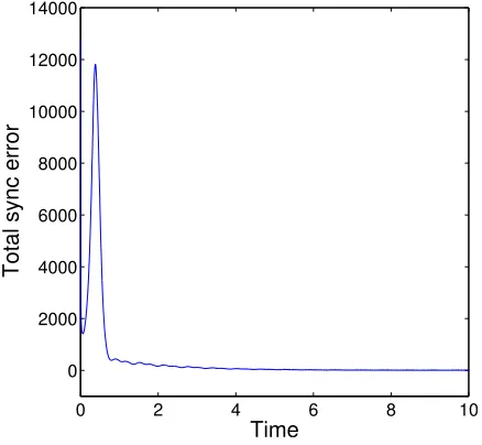
Then, the timetis recorded as the synchronized time. One typical case of synchronization performance is shown in Figure2, which displays only thex-variables of 20 randomly selected nodes from the network of 200 nodes, witha¼50,c¼12, andr¼2.5, plotted on the time interval

½0;1. The total sync error is defined by

E¼X

i;j

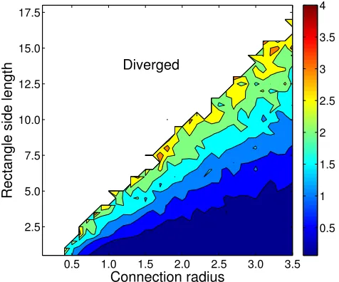
jjxixjjj2: (22)

The most interesting situations emerge when we study the synchronization time as a function of both the connection radiusrand the rectangle side lengtha. In Figure3, we show the results where the synchronization time is contour plotted as a function ofranda. The first clear observation is the exis-tence of a region (in white color in Figure3) where synchroni-zation of the system is not achievable. This region corresponds to very elongated rectangles for a given connec-tion radius, as predicted by the theory above. For instance, the synchronization process for a RRG with connection radius r¼2.0 and rectangle side lengtha>10 is not achievable. The main cause for the divergence in the synchronization time is that the RRG becomes disconnected for a corresponding

radius as the rectangle becomes extremely elongated (see (3) and Ref.12).

Another interesting observation is that for a given side lengtha>1, which generates a rectangle, the synchroniza-tion time decays as the connecsynchroniza-tion radius increases. This is an expected result because increasing the connection radius makes the RRG more densely connected, approaching a complete graph in the limit. However, as we have found ana-lytically (see (19)), the elongation of the rectangle makes the network less synchronizable. That is, for a given node num-bernand connection radiusr, the eigenratioQdepends only ona, and becauseQð8_að Þ4ar_þ12Þlog

2

2n;asa! 1, the eigenra-tioQ!0, which implies that the network is poorly synchro-nizable. In Figure3, it can be seen that for a given value ofr, the synchronization time increase asaincreases, i.e., going from bottom to top of the plot, and at a certain point the syn-chronization time diverges due to the network disconnection. The structural causes, explaining this increase in the syn-chronization time with the increase of the rectangular side length, can be resumed as follows. Asa! 1,

• _{The average degree of the nodes in a RRG decays}

accord-ing to the results given in Theorem 1;

• _{The average path length in a RRG grows to infinity}

according to the results given in Proposition 4. Also, the diameter of the graph increases as we have seen in Theorem 7;

• _{The probability that a RRG becomes disconnected}

increases according to the results given in Proposition 2.

These three structural properties have significant influ-ences on the synchronizability of the resulting RRGs. These results show that as the rectangle becomes more elongated, the resulting RRG becomes less densely connected, less “small-world”-like, and more prone to be disconnected. All

of which make the synchronization process more difficult to converge.

As we have reported previously (see Ref.12), the aver-age clustering coefficient follows a non-monotonic behavior with the increase of a. A RRG first becomes more clustered as the rectangle elongates, and after a certain critical value, the clustering decays almost linearly with the subsequent in-crement ofa. Thus, it is possible that this initial increase of the clustering attenuates the loss of the synchronizability of a RRG for relatively small values ofa.

The region of better synchronizability for the RRGs here appears to be demarcated by an approximate straight line: a¼2r0:83 (see the deep blue lower triangle in Figure3). This means that for a network with the size studied here, a good synchronization is reached if

aþ0:83 r <2:

VII. CONCLUSIONS

This paper studies the synchronizability of a recently proposed RRG network model, deriving analytically the upper and lower bounds of the eigenratio of the network Laplacian matrix. RRGs account for the spatial distribution of nodes allowing the variation of the shape of the unit square commonly used in RGGs. The paper also investigates the synchronization processing of representative RRG net-works with nodes being chaotic Lorenz systems, showing complete consistence with the theoretical results. The new RRG model has some attractive theoretical and practical fea-tures that deserve further investigation in the near future, including its controllability, observability, identifiability, and potential real-world applications.

ACKNOWLEDGMENTS

This research was supported by a Wolfson Research Merit Award from the Royal Society (EE) and by the Hong Kong Research Grants Council under the GRF Grant CityU-11201414 (GC).

1

N. Alon and V. D. Milman, “k1isoperimetric inequalities for graphs and

superconcentrators,”J. Comb. Theory B38, 73–88 (1985).

2_{A. Arenas, A. Dıaz-Guilera, J. Kurths, Y. Moreno, and C. Zhou,}

“Synchronization in complex networks,”Phys. Rep.469, 93–153 (2008).

3

A.-L. Barabasi and R. Albert, “Emergence of scaling in random networks,”Science286, 509–512 (1999).

4

M. Barahona and L. M. Pecora, “Synchronization in small-world systems,” Phys. Rev. Lett.89, 054101 (2002).

5_{G. Chen and Z. Duan, “Network synchronizability analysis: A}

graph-theoretic approach,”Chaos18(3), 037102 (2008).

6

G. Chen, X. F. Wang, and X. Li, Fundamentals of Complex Networks: Models, Structures and Dynamics(Wiley, 2015).

7_{J. Dall and M. Christensen, “Random geometric graphs,”Phys. Rev. E}

66, 016121 (2002).

8_{A. Dıaz-Guilera, J. Gomez-Garde~nes, Y. Moreno, and M. Nekovee,}

“Synchronization in random geometric graphs,”Int. J. Bifurcation Chaos 19, 687–693 (2009).

9_{F. D€orfler, M. Chertkov, and F. Bullo, “Synchronization in complex}

oscil-lator networks and smart grids,” Proc. Natl. Acad. Sci. U. S. A. 110, 2005–2010 (2013).

10_{P. Erd€os and A. Renyi, “On the evolution of random graphs,” Pub. Math.}

Inst. Hung. Acad. Sci.5(1), 17–60 (1960). FIG. 3. Dependence of the synchronization time on both the connection

11

E. Estrada,The Structure of Complex Networks: Theory and Applications (Oxford University Press, 2011).

12

E. Estrada and M. Sheerin, “Random rectangular graphs,” Phys. Rev. E 91, 042805 (2015); e-printarXiv:1502.0257.

13_{H. Kenniche and V. Ravelomananana, “Random geometric graphs as model}

of wireless sensor networks,” in the 2nd IEEE International Conference on Computer and Automation Engineering (ICCAE, 2010), Vol. 4.

14_{C. W. Wu,Synchronization in Complex Networks of Nonlinear Dynamical}

Systems(World Scientific Publishing Company, 2007).

15

Y.-Y. Liu, J.-J. Slotine, and A.-L. Barabasi, “Controllability of complex networks,”Nature473, 167–173 (2011).

16_{E. N. Lorenz, “Deterministic nonperiodic flow,” J. Atmos. Sci. 20,}

130–141 (1963).

17

A. E. Motter, C. Zhou, and J. Kurths, “Network synchronization, diffu-sion, and the paradox of heterogeneity,” Phys. Rev. E 71, 016116 (2005).

18

M. W. Newman, “The Laplacian spectrum of graphs,” M.S. thesis (University of Manitoba, 2000).

19

M. D. Penrose, Random Geometric Graphs (Oxford University Press, 2003).

20_{A. Trafton, “Synchronized brain waves enable rapid learning,” MIT News,}

June 2014; see http://newsoffice.mit.edu/2014/synchronized-brain-waves-enable-rapid-learning-0612.

21_{X. F. Wang and G. Chen, “Synchronization in small-world dynamical}

networks,”Int. J. Bifurcation Chaos12, 187–192 (2002).

22

X. F. Wang and G. Chen, “Synchronization in scale-free dynamical net-works: Robustness and fragility,”IEEE Trans. Circuits Syst. 49, 54–62 (2002).

23_{D. J. Watts and S. H. Strogatz, “Collective dynamics of ‘small-world’}

networks,”Nature393, 440–442 (1998).

24