Adaptive Video Compression using PCA Method

Adaptive Video Compression using PCA Method

Mostafa Mofarreh-Bonab

Department of Electrical and Computer Engineering Shahid Beheshti University,Tehran, Iran

Mohamad Mofarreh-Bonab

Electrical and Electronic Engineering school, University of Bonab, East Azerbaijan, Iran

ABSTRACT

In this paper, a new PCA based method for video compression is introduced. This method extracts the features of video frames and process them adaptively based on required accuracy. This idea improves the quality of compression effectively. In this paper, we focused on the fact that video is a composition of sequential and correlated frames, so we can apply the PCA to these high correlated frames. Most of other video compression methods use DCT transform to compression. DCT causes to large damage in the edges of frames which plays fundamental role in quality of video. Our method in this paper doesn’t reduce the bandwidth of frequency response, so the edges of frames don’t fade.

Keywords

Video Compression, Correlation, PCA, SVD, 2DPCA, Frame, Feature extraction, Database, PSNR, Bit Rate.

1.

INTRODUCTION

PCA -also known as KL Transform for images- is a statistical approach which is used widely in pattern recognition and compression of various type of databases, especially image databases which their components have high correlation -i.e. frontal face databases. This method first used by Kirby and Sirovich for compressing human face image database [7], [8].In PCA method, features of images are extracted by means of images correlations and these information are mapped to an orthogonal space and the features that are correspond to less important components -smaller eigenvalues- are ignored. In this approach, compression is reached by very little loss of information [1]. In fact, the eigenvectors and their corresponding eigenvalues are extracted using the covariance matrix of images. Since the eigenvectors which are related to small eigenvalues have very low information, their elimination has almost no effect on the quality of reconstructed images and compression is done by eliminating those components. There are other Optimal PCA-based methods for compressing images which show better results than conventional PCA, i.e. 2DPCA, K2DPCA, KPCA, L1-norm-Based2DPCA and so on[3], [11], [10], [9]. As mentioned in the following, a combination of improved PCA presented by M.Mofarreh et.al. in [1] and the introduced method in [2] for compressing one image show better results rather than other methods. Also we will show that other PCA based methods don’t have proper performance for video sequences.

2.

PCA method

Suppose there areMgrayscale N × Pimages. N × Pgrayscale images are equivalent to N × P matrixes that the values of the components of the matrixes are the light intensities of the corresponding pixel's location. Put N × P = Q. By reshaping the matrixes, the image can be expressed as 1 × Qvectors Fiin equation 1. Applying PCA, images are transferred to another field. All images are put in 𝑿 matrix that its elements are the intensity values of images.

𝐗 = F1

⋮ FM _M×Q

, Fi= xi1, xi2, … , xiQ _1×Q Eq. 1

The term Fi indicates the ith image which is converted to a vector. In order to applying PCA, some definitions should be considered;

The mean vector, Mx: that contains mean values of each image and expressed as:

Mx=_Q1

Qk=1x1k x2k Q k=1

. .

xMk Q

k=1 M×1

= m1 m2 . . . mM

Eq. 2

𝐌x matrix, that contains the values of Mx for 𝑀 times and expressed as:

𝐌x= [Mx, Mx, … , Mx]M×Q Eq. 3 Covariance matrix 𝐂x for 𝑀 rows of 𝑿 matrixis [1]: 𝐂x= ci,j_M×M

That: ci,j=_{Q − 1}1 ×

xik− Mx i, 1 × (xjk− Mx(j, 1)) Q

k=1 Eq. 4

For 𝐂𝐱 matrix, 𝑀eigenvectors vi , i = 1,2, … , M and 𝑀 eigenvalues λi , i = 1,2, … , M can be found, which satisfy equation 5:

∀i ∈ 1,2, … , M , , Cx. vi= λi. vi

vi= v1(i) v2(i) ⋮ vM(i)

Eq. 5

The modal matrix 𝚲 will be obtained by putting all eigenvectors in a matrix, that its columns are the eigenvectors of Cx as shown below [2]:

𝚲 = [v1, v2, … , vM] Eq. 6 Now we can define 𝑽 matrix:

𝐕 = 𝚲−1 _{Eq. 7}

𝚲is a unitary matrix. So:

𝚲−1_{= 𝚲}T_{⟹ 𝐕 = 𝚲}T _{Eq. 8}

𝐕 = v1(1) ⋯ v⋮ ⋱ M⋮(1) v1(M) ⋯ vM(M) M×M

Eq.10

Applying PCA produces 𝒀 matrix:

𝐘 = 𝐕. 𝐗 − 𝐌x Eq. 11

with ,𝐕 and 𝐌x matrixes and inversing mentioned process, 𝐗matrix can be calculated as equation 12:

𝐘 = 𝐕. 𝐗 − 𝐌x ⇒ 𝐕−1. 𝐘 = 𝐗 − 𝐌x ⇒ 𝐗 = 𝐕−1_{. 𝐘 + 𝐌}

x Eq. 12

According to equation 8 we can write:

𝐕−1_{= (𝚲}T₎−1_{= (𝚲}−1₎−1_{= 𝚲 = 𝐕}T _{Eq. 13} Now,𝐗matrix can be retrieved using equation 14: 𝐗 = 𝐕T_{. 𝐘 + 𝐌}

x Eq. 14

For compressing 𝐗, some definitions are made as below[3]: 𝐕k ≜ v1, v2, … , vk T_M×k, k ∈ {1,2, … , M} Eq. 15

𝐘k≜

Y 1,1 ⋯ Y(1, Q)

⋮ ⋱ ⋮

Y(k, 1) ⋯ Y(k, Q)_k×Q Eq.16 𝐗 ≜ 𝐕kT. 𝐘k+ 𝐌x Eq. 17 Considering the first k Eigen vectors from the M Eigen vectors (K<M), the 𝐗 matrix that is slightly different from𝐗 matrix, can be retrieved.

The 𝐗 matrix is compressed matrix which obtained from 𝐗. So the compression ratio - the ratio of the required memory to save𝐗 to the required memory to save 𝐗 - can be calculated as equation 18 shows:

Memoryratio =requiredmemorytosave 𝐗 requiredmemorytosave 𝐗

≜mem 1_{mem 2} Eq. 18

mem1is the required memory to save 𝐕kT, 𝐘k, 𝐌x. mem2is the required memory to save 𝐗.

⟹ Memoryratio =kM +kQ +M_MQ Eq. 19

3.

IMPROVED PCA:

M. Mofarreh et.al. in [1] show that, it is possible to address the most erroneous pixels in the reconstructed images and improve the quality of images exactly at those pixels. According to [1], the 𝐘k matrix is converted to 𝐘 k as Eq. 20, which nonzero columns in the bottom of the matrix are applied to compensate the effect of error:

𝐘 k=

Y(1,1) ⋯ Y(1, α) ⋯ Y(1, N2_{− 1) Y(1, N}2₎

Y(2,1) ⋯ Y(2, α) ⋯ Y(2, N2_{− 1) Y(2, N}2₎

⋮ ⋮ ⋮ ⋮ ⋮ ⋮

Y(k, 1) ⋯ Y(k, α) ⋯ Y(k, N2_{− 1) Y(k, N}2₎

0 0 Y(k + 1, α) ⋯ 0 0 0 0 Y(k + 2, α) ⋯ 0 0

⋮ ⋮ ⋮ ⋮ 0 0

0 0 Y(M, α) ⋯ 0 0 _M×N2

Eq. 20

4.

2DPCA Method:

For applying PCA method, all image matrixes should be converted to vectors previously, so the resulting image vectors of images construct a high dimensional image vector space which its complexity doesn’t let accurate enough calculations of covariance matrixes. 2DPCA technique uses 2D matrixes rather than 1D vectors in conventional PCA and this idea leads to smaller matrix spaces rather than high dimensional vectors. In fact, in 2DPCA technique, an image covariance matrix which its size is much smaller than covariance matrix of PCA is generated directly from image matrixes. So 2DPCA has two fundamental advantages over conventional PCA: easily construction of accurate covariance matrixes and smaller required time to calculate corresponding eigenvectors - because of the smaller size of covariance matrixes-. Suppose𝐀 is an N × P image and X is a P-dimensional unitary column vector. Projecting A onto X by the linear transformation Y = 𝐀. X leads to produce an N-dimensional projected vectorY that is called the projected feature vector of image 𝐀.the goal of 2DPCAis to find the proper projection vector X. from this point of view, following criterion is adopted:

J 𝐗 = tr 𝐒x Eq. 21

That 𝐒x is the covariance matrix of the projected feature vectors of the training samples and tr 𝐒x is the trace of 𝐒x. Maximizing the criterion in 21 leads to find a projection direction X, so that the total scatter of the resulting projected samples is maximized.

The covariance matrix 𝐒x is defined as: 𝐒x= E Y − EY Y − EY

T

= E 𝐀X − E(𝐀X) 𝐀X − E(𝐀X) T

= E 𝐀 − E𝐀 X 𝐀 − E𝐀 X T Eq. 22 So, tr(𝐒x) = XT E 𝐀 − E𝐀

T

𝐀 − E𝐀 X Eq. 23 Let 𝐆t= E 𝐀 − E𝐀

T

𝐀 − E𝐀 .

𝐆tis called the image covariance matrix and is a P × Pnonnegative definite matrix and can retrieved directly using the training image samples.

Suppose there are M images. Jth image is expressed by 𝐀j , j = 1,2, … , M which is a N × P matrix. Let show the mean image of all images with 𝐀, so the 𝐆t matrix can be expressed as:

𝐆t=_M1 𝐀Mj=1 j− 𝐀 T 𝐀𝐣− 𝐀 Eq. 24 And criterion 21 can be written as:

J X = XT_𝐆

tX Eq. 25

eigenvectors of 𝐆𝐭 that have largest corresponding eigenvalues.

Optimal projection vectors are used to extracting features of images. For a sample image 𝐀 projected feature vectors are: Yk= 𝐀Xk, k = 1,2, … , d Eq. 26 So, a set of projected feature vectors for image 𝐀 are obtained that called principal components (vectors) of the image. Note that the principal components in 2DPCA are vectors, in oppose with conventional PCA which their principal components were scalars.

Obtained principal vectors are used to build a N × d matrix that is called feature matrix or feature image as below:

𝐁 = Y1, … , Yd Eq. 27

5.

2DPCA based Image Reconstruction

Principal components and eigenvectors (eigenfaces) are used to reconstruct images in PCA. Equivalently, in 2DPCA we retrieve images as following approach:

Suppose d orthonormal eigenvectors which correspond to d largest values of eigenvectors of covariance matrix 𝐆t are X1, X2, … , Xd. After projecting image onto these d axes, resulted principal component vectors are:

Yk= 𝐀Xk, k = 1,2, … , d Eq. 28 Now, let 𝐕 = Y, … , Yd and 𝐔 = X1, … , Xd , so:

𝐕 = 𝐀. 𝐔 Eq. 29

Since X1, … , Xd are orthonormal vectors, so we can reconstruct the image 𝐀 easily. We call this reconstructed image 𝐀 which is calculated as below:

𝐀 = 𝐕𝐔T_{= Y} kXkT d

k=1 Eq. 30

Suppose:

𝐀k= YkXkT, k = 1,2, … , d Eq. 31 Note that the size of 𝐀k is the same size of 𝐀 and called a subimage of 𝐀. A combination of d subimages can reconstruct the image 𝐀. If the number of principal components are d = P, no information will be lost and 𝐀 = 𝐀. But if the number of principal components are less than P, i.e. d < 𝑃, some information have been lost and 𝐀 will be an estimation of 𝐀.

6.

Improved PCA and 2DPCA for Video

In this section, the results of applying three mentioned methods: PCA, Improved PCA and 2DPCA for compression of 14 sample frames are presented. The frames are chosen from throwing an apple in a white background. Figure 1 shows the original frames. The frames are arranged from the top down and left to right.

Fig 1: Original frames

Based on our background on PCA, 2DPCA and improved PCA in face database compression, we expect that 2DPCA will provide the best performance in video compression too but according to simulations, the improved PCA shows better results than two other methods. Figure.2 shows the first three frames of applying mentioned triple methods with same bitrates to the original frames. As it seen, the PCA method added fade effects to the reconstructed frames and applying 2DPCA causes vertical lines and black bands to the frames. So in this application (video compression), the best performance is provided by improved PCA method.

a b c

Fig 2: a) PCA, b) Improved PCA, c) 2DPCA (Note to the vertical lines and black bands on the right

side of 2DPCA results)

7.

Mentioned Method

frames have sharp variations. As an example figure 3 represents 3 frames of a video. As it seen, some sections of these frames are constant in 3 frames.

Fig 3: 3 sample frames to show constant and moving parts of the frames

Suppose 3 frames are 3 images. We apply PCA after converting them to vectors. As it investigated in the previous sections, PCA has some weaknesses in compression of images that belong to a moving object, so for improving the quality of erroneous pixels we should to increase the value of k, which in turn causes to unnecessary increase in other constant parts ofthe frame and this reduces the overall performance of method. For increasing the quality of moving parts of frames, we divided the frames in some bands, so we can apply the PCA to these bands separately. By this idea, constant and moving parts of frames have been separated from each other, so we can save constant parts of frames using little number of eigenfaces and save moving parts using more eigenfaces. This concept done by getting feedback from conventional PCA. Figure 4 shows the designed Encoder.

Fig 4: Block Diagram of designed Encoder for mentioned method

N Sub Videos With M images

Input Video

Sequence

(S×T)

First Sub Video

with M frames

Nth Sub Video

with M frames

Pth band of sub video

PCA

PCA

Fist band of sub video

Pth _{band of sub video}

PCA

PCA

Fist band of sub video

Fig 5: Diagram of designed Encoder for mentioned method, continued

Mentioned method is applied to video as follows:

1. Dividing input video to 𝑁 subvideos that each subvideo has 𝑀 frames

2. Dividing all subvideos to 𝑃 bands with equal width 3. Converting 𝑁 × 𝑃 obtained frame groups to vectors

and constructing 𝑿 matrix. In fact, there are 𝑁 × 𝑃, 𝑿 matrixes.

4. Applying PCA to all 𝑁 × 𝑃 groups, according to required SSIM value. For each group, required number of eigenfaces should be saved.

5. Getting feedback of reconstructed frames and correcting most erroneous pixels according to SSIM.

6. Saving all 𝒀𝑘 and 𝑽𝑘matrixes.

One of the advantages of this method is the simplicity of its decoding procedure. The decoding procedure is as figure 6:

Fig 6: Designed Decoder for mentioned method

As figure 6 shows, decoding of coded information is done in a simple way. The required calculations for decoding a 𝑅 × 𝑆video with 𝑁 × 𝑀 frames that each frame is splitted to 𝑃 bands are as equation 32:

𝑿

= 𝒗𝑀×𝑀𝑇 . 𝒀_{𝑘 𝑘×(}𝑅

𝑃×𝑆)+ 𝑴𝑥 𝑀×( 𝑅 𝑃×𝑆)

Eq. 32

𝑣𝑘 , 𝑌𝑘 , 𝑀𝑥

𝑣𝑘 , 𝑌𝑘 , 𝑀𝑥

First band

Mth band

Pth band of sub video

Reconstructed

video

𝑋 = 𝑣_𝑘−1_{. 𝑌}

𝑘+ 𝑀𝑥

𝑋 = 𝑣𝑘−1. 𝑌𝑘+ 𝑀𝑥

X = 𝐹𝑖𝑟𝑠𝑡 𝑣𝑒𝑐𝑡𝑜𝑟⋮ 𝑀𝑡ℎ _{𝑣𝑒𝑐𝑡𝑜𝑟} Pth band of sub video

First band

Second band

Mth _band

Mth vector Second vector

First vector

Applying KL Transform and derivation of V and Y and 𝑀𝑥

Put: 𝑘 = 𝑘0 and calculate the the reconstructed bands and : 𝑡 =

𝑀𝑖𝑛𝑖𝑚𝑢𝑚 𝑆𝑆𝐼𝑀 𝑏𝑒𝑡𝑤𝑒𝑒𝑛 𝑟𝑒𝑐𝑜𝑛𝑠𝑡𝑟𝑢𝑐𝑡𝑒𝑑 𝑏𝑎𝑛𝑑𝑠 𝑎𝑛𝑑 𝑖𝑛𝑝𝑢𝑡 𝑏𝑎𝑛𝑑𝑠

Yes

𝑡 > 𝑡₀ ? _𝑘

0= 𝑘0+ 1

Save

𝑣

, 𝑌

, 𝑀

According to equation 32, it’s clear that only adders and multipliers are needed for this decoder.

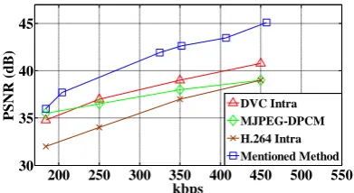
In contrast with other famous video compression methods like DVC Intra, H.264 Intra and MJPEG-DPCM, mentioned method in this paper provides better performance and less complexity, as represented in fig 7.

Fig 7: Curves of some low complexity encoders for video Compression applied to Akiyo frames

In order to illustrate the adaptively of mentioned method, note to two following frames which are first and 10th frames of 300 frames of Akiyo video sequence available at media.xiph.org/video/derf online at figure 8. These frames are divided into 8 bands and as it clear in figure 8, the bands 1, 2, 3 , 5, 6, 7 and 8 are almost constant and its only the 4th band that changes. For compression with a distinct SSIM value for 50 frames, using a few numbers of eigenfaces for constant parts satisfies the quality requirements and it’s necessary for variable parts to use more eigenfaces. The number of needed eigenfaces can be calculated by mentioned algorithm in previous sections.

8.

ACKNOWLEDGMENTS

The authors would like to thank the reviewers for their beneficial comments and suggestions.

9.

CONCLUSION

In this paper, PCA method is analyzed for video compression. Some other methods based on PCA like 2DPCA are also investigated and we showed that although they are high performance in face database compression but in video compression they didn’t show such good performance.

Mentioned method in this paper has several advantages like more simplicity in encoder and especially in decoder, because of using just adders and multipliers in their structures -in oppose to the other methods which use more complicated functions like inverse FFT and motion estimation functions-.

10.

REFERENCES

[1] Mostafa Bonab and Mohamad Mofarreh-Bonab, “Face Database Compression By Hotelling Transform Using A New Method,” 2nd _World Conference on Information Technology, 23-27 Nov. 2011, Antalya, Turkey.

[2] Mohamad Bonab and Mostafa Mofarreh-Bonab, “A New Technique For Image Compression Using PCA,” International Journal of Computer Science and Communication Networks, IJCSCN, vol. 2, pp. 111-116, 2012.

[3] J. Yang, D. Zhang, A. F. Frangi and J.Y. Yang, “Two-Dimensional PCA: A New Approach to Appearance-Based Face Representation and Recognition,” IEEE Trans. Pattern Analysis and Machine Intelligence, vol. 26, No. 1, pp. 131-137, 2004

[4] Z. Gu, W. Lin, B. Lee, C. Lau, “Low-Complexity Video Coding Based on Two-Dimensional Singular Value Decomposition,” IEEE Trans. Image Processing, vol. 21, No. 2, pp. 674-687, Feb 2012.

[5] A.M. Aznaveh, F. Torkamani Azar, A. Mansouri, “Face Database Compression by Hotelling Transform Using Segmentation, Signal Processing and Its Applications, 2007. ISSPA 2007.

[6] L. I. Smith, “A Tutorial on Principal Component

Analysis [online], Available:

csnet.otago.ac.nz/cosc453/student_tutorials/principal_co mponents.pdf, 2002

[7] L. Sirovich and M. Kirby, “ Low-Dimensional Procedure for Characterization of Human Faces,” J. Optical Soc. Am., vol. 4, pp. 519-524, 1987.

[8] M. Kirby and L. Sirovich, “Application of the KL Procedure for the Characterization of Human Faces,” IEEE Trans. Pattern Analysis and Machine Intelligence, vol. 12, no. 1, pp. 103-108, Jan. 1990.

[9] X. Li, Y. Pang, Y. Yuan, “L1-Norm-Based 2DPCA,” IEEE Trans. Systems Man and Cybernetics, vol. 40, No. 4, 2009.

[10]Y. Li, X. Lei, B. Bai and Y. Zhang, “Information Compression and Speckle Reduction for Multi Frequency Polarimetric SAR Images Based on Kernel PCA,” Journal of Systems Engineering and Electronics, vol. 19, pp. 493-498, 2008.

[11]C. Yu, H. Qing and L. Zhang, “K2DPCA plus 2DPCA: An Efficient Approach for Appearance Based Object Recognition”, 3rd

International Conference on Bioinformatics and Biomedical Engineering, ICBBE, 2009.

200 250 300 350 400 450 500 550

30 35 40 45

P

S

N

R

(d

B)

kbps

DVC Intra MJPEG-DPCM H.264 Intra Mentioned Method