Theses
Thesis/Dissertation Collections
11-20-2015
Semi-Supervised Pattern Recognition and Machine
Learning for Eye-Tracking
Thomas B. Kinsman
Follow this and additional works at:
http://scholarworks.rit.edu/theses
This Dissertation is brought to you for free and open access by the Thesis/Dissertation Collections at RIT Scholar Works. It has been accepted for inclusion in Theses by an authorized administrator of RIT Scholar Works. For more information, please [email protected].
Recommended Citation
Eye-Tracking
by
Thomas B. Kinsman
B.S.E.E. University of Delaware, 1983 M.S.E.C.E. Carnegie Mellon University, 1987
A dissertation submitted in partial fulfillment of the requirements for the degree of Doctor of Philosophy in the Chester F. Carlson Center for Imaging Science
College of Science
Rochester Institute of Technology
November 20, 2015
Signature of the Author
Accepted by
ROCHESTER INSTITUTE OF TECHNOLOGY ROCHESTER, NEW YORK
CERTIFICATE OF APPROVAL
Ph.D. DEGREE DISSERTATION
The Ph.D. Degree Dissertation of Thomas B. Kinsman has been examined and approved by the
dissertation committee as satisfactory for the dissertation required for the
Ph.D. degree in Imaging Science
Dr. JeffPelz, Dissertation Advisor
Dr. Mark Fairchild
Dr. Nathan Cahill
Dr. Carol Romanowski
Date
ROCHESTER INSTITUTE OF TECHNOLOGY
CHESTER F. CARLSON CENTER FOR IMAGING SCIENCE
Title of Dissertation:
Semi-Supervised Pattern Recognition and Machine Learning for Eye-Tracking
I, Thomas B. Kinsman, hereby grant permission to Wallace Memorial Library of R.I.T. to reproduce my thesis in whole or in part. Any reproduction will not be for commercial use or profit.
Signature
Date
by
Thomas B. Kinsman Submitted to the
Chester F. Carlson Center for Imaging Science in partial fulfillment of the requirements
for the Doctor of Philosophy Degree at the Rochester Institute of Technology
Abstract
The first step in monitoring an observer’s eye gaze is identifying and locating the image of their pupils in video recordings of their eyes. Current systems work under a range of conditions, but fail in bright sunlight and rapidly varying illumination. A computer vision system was developed to assist with the recognition of the pupil in every frame of a video, in spite of the presence of strong first-surface reflections offof the cornea.
A modified Hough Circle detector was developed that incorporates knowledge that the pupil is darker than the surrounding iris of the eye, and is able to detect imperfect circles, partial circles, and ellipses. As part of processing the image is modified to com-pensate for the distortion of the pupil caused by the out-of-plane rotation of the eye. A sophisticated noise cleaning technique was developed to mitigate first surface reflec-tions, enhance edge contrast, and reduce image flare. Semi-supervised human input and validation is used to train the algorithm.
The final results are comparable to those achieved using a human analyst, but require only a tenth of the human interaction.
First and foremost I must acknowledge the love and support of my wife, Lynn E. Kinsman. Lynn adds much needed order to the chaos of my life. Both spiritually and financially, she has kept the family growing and the house running. Lynn proof-read several chapters of my proposal, kept the family together, supervised college visits for our oldest child, and supported me spiritually during the entire thesis processes. Lynn is my soul mate.
JeffB. Pelz has been my steadfast adviser throughout the process, providing guidance and financial and academic support and encouragement over the years. For me it was not just a journey of finding the solutions, it was also a journey of understanding the methods well enough to teach them in the future. Jeffsupported me in this, went to bat for me, fought more political arguments than I am aware of, and encouraged me to go out into the world and profess. Jeffis a friend and a confidant, and through his confidence in me I have gained wisdom.
Mark D. Fairchild was my first professor at RIT. Mark is a wonderful example of a dedicated professor and collaborator. I use some of his teaching methods to this day. We share an interest in furthering the state of education, the vision system, and anomalous-trichromacy.
I am sincerely grateful to Nathan D. Cahill. Nate gave guidance and inspiration throughout the process. Nate encouraged me to take advantage of the constrained nature and motions of the eye, and to develop the method for unwrapping the eye. Nate also provided additional guidance on the structure of this dissertation.
Carol Romanowski was my first graduate professor, and taught the first course I took in machine learning and data mining. In a sense she was behind me “before the beginning” of my Ph.D. journey. Now as I teach one of the classes that she taught, I constantly think of how she taught them. Carol is a source of guidance in all things, and I am extremely fortunate to have her serving on my committee. I am deeply indebted to Carol for her thorough review of this work and her many useful and enlightening comments. This thesis reads much better because of her, and I owe her a great debt.
Many people at RIT helped me navigate academic administration. These people include Sue Chan who assured that my coursework was on track, and Joyce French who kept my finances in order. Joe Pow is always at the center of the Center for Imaging Science. I would also like to thank Val Hemink, Mel Warren, Beth Lockwood and many others that helped on a day-to-day basis.
I would like to thank my parents, Betty and Bill, for their love and support, and for being good role models. I would like to thank my children, Duncan and Devon, for putting up with my long hours away as I tried to set a good role model. Again, I want to thank my wife, Lynn, or keeping the family happy and healthy.
I would like to thank John Kerekes and Anthony Vodacek for admitting me to the program. Dr. Kerekes also serves as the Ph.D. program coordinator, and Dr. Vodacek served as another adviser. They both provided the different point of view that was sometimes needed to see through noise.
I would also like to thank Mar`ıa Helguera for her help, support, and advice over the years. Dr. Helguera’s medical imaging classes emphasized the importance of contrast in any feature used for computer vision or machine learning.
I would like to thank Juan Cockburn, Harvey Rhody, Roger Gaborski, and Rox-anne Canosa for numerous discussions of computer vision. Carl Salvaggio, Naval Rao, Jan van Aardt, and Peter Bajorski were also helpful for clarifying discussions on topics from LiDAR to statistics. Thanks are due to Roger Easton for periodic sessions on imaging mathematics, and to Emmett Ientilucci for additional tutoring on radiometry.
There are many students to thank. These include my study mates Brandon May and Kelly Canham. Office mates and the entire cadre of students that I went through the core courses with. Michael Presnar, Karl Walli, Jarad Herweg, and Brian Flusche were especially helpful. I also wish to thank the other graduate students in the Multidisci-plinary Vision Research Laboratory, Susan Munn, Tommy Keane, Dong Wang, Preeti Vaidynathan, and Kate Walders.
Since research is a critical part of a Ph.D. quest, many of the staffof the Wallace library became colleagues. Most of the research librarians, especially Adwoa Boateng, Susan Mee, Linette Koren, Roman Koshykar, and Gus Kovalik knew me on a first name basis. Internet searches cannot reliably answer a question about the interaction of artwork and human vision, but Kari Horowicz can.
The Wallace Center also includes some helpers behind the scenes who should be known to those that follow. Tracey Melville and Diane Grabowski are in charge of thesis and dissertation binding. If you are not reading this in a bound form, but are instead reading it electronically, it is because of Jennifer Roeszies, the coordinator for electronic dissertations. Another secret super-hero for research is Morna Hilderbrand, Interlibrary Loan Librarian and Manager for the IDS Department. Morna Hilderbrand never failed to obtain any book or reference. Morna and her team connect the Wallace library to a network of libraries throughout US and beyond.
Contents
Declaration . . . 1
Approval . . . 2
Copywrite . . . 3
Abstract. . . 4
Acknowledgements . . . 5
Dedication . . . 8
List of Figures 16 List of Tables 20 1 Introduction 22 1.1 Problem Statement . . . 23
1.1.1 System Requirements . . . 24
1.1.2 Calibration. . . 24
1.1.3 Mobile Eye Tracking Requirements . . . 25
1.2 Data Inundation Problems and Issues . . . 25
1.2.1 Data Inundation in Frames . . . 25
1.2.2 Data Inundation in Pixels . . . 26
1.2.3 Yarbus Software. . . 26
1.2.4 Data Reduction Techniques for Analysis. . . 27
1.2.5 Pupil Location. . . 27
1.3 Processing Stages . . . 28
1.3.1 Automated Approach . . . 28
1.3.2 Use of Semi-Supervised Learning . . . 29
1.4 Innovations . . . 30
2 Workflow and Primary Passes 33 2.1 Overview of Primary Processing Passes . . . 34
2.2 First Pass and Statistical Collection . . . 36
2.2.1 Background Removal Statistics . . . 36
2.2.2 Blink Detection Statistics and Algorithm . . . 37
2.2.3 Stable Frame Identification . . . 38
2.3 Easy-Pupil Detection Pass . . . 39
2.4 First User Validation Pass . . . 40
2.4.1 Establishing Ground Truth Pupils . . . 41
2.4.2 Establishing GroundFalsePupils . . . 42
2.5 Modeling . . . 42
2.5.1 Edge Strength Modeling . . . 42
2.5.2 Eye Geometry Modeling . . . 42
2.6 Automatic Pupil Detection Pass . . . 43
2.7 Final Inspection . . . 44
2.8 Summary . . . 44
3 Eyelid Location and Removal 46 3.1 Overview. . . 46
3.2 Edge Detection for Eyelid Location . . . 48
3.3 Lower Eyelid Detection . . . 49
3.4 Upper Eyelid Detection. . . 51
3.5 Example Results . . . 54
3.6 Numerical Results. . . 57
3.7 Conclusions about Eyelids . . . 57
4 Adaptive Edge Preserving Noise Reduction for Pupils 59 4.1 Introduction . . . 59
4.2 Adaptive Processing . . . 59
4.3 Background Importance of Data . . . 60
4.3.1 Pupil Detection Approaches. . . 62
4.4 A Taxonomy of Edges . . . 63
4.5 The Resolution Challenge . . . 64
4.6 Noise Sources . . . 64
4.6.1 Structured Noise . . . 65
4.6.2 Compression Artifacts . . . 65
4.6.3 Variations Across Subjects . . . 66
4.6.4 Within Video Variations . . . 67
4.6.5 Sudden Changes in Illumination . . . 67
4.6.6 Additional Noise Edge Sources . . . 68
4.7 Standard Noise Removal Methods . . . 68
4.7.1 Gaussian Filtering . . . 68
4.7.2 Median Filtering . . . 68
4.7.3 Comparison to the Method Used . . . 69
4.7.5 Other Methods . . . 71
4.8 An Adaptive Noise Removal For Edge Detection . . . 72
4.8.1 Leveraging Duality of Segmentation and Edge Detection . . . 72
4.9 An Adaptive Edge Preserving Filter . . . 72
4.9.1 Example Algorithm Using Eight Regions . . . 73
4.9.2 Comparison in One Dimension . . . 74
4.9.3 The Secret of the Shapes . . . 76
4.10 Performance Optimization . . . 81
4.10.1 Fast Variance Computation . . . 81
4.10.2 Algorithm in Pseudocode . . . 82
4.10.3 Re-weighting the Variance. . . 83
4.10.4 Failure Modes . . . 85
4.11 Additional Benefits . . . 85
4.11.1 Edge Enhancement in Transition Regions . . . 85
4.11.2 Edge Direction . . . 86
4.12 Results – Before and After Images . . . 86
4.13 Comparison to Other Methods . . . 96
4.13.1 Unsharp Masking. . . 96
4.13.2 Bilateral Edge Detection . . . 96
4.14 Conclusions . . . 98
5 The Hough Transform 100 5.1 Overview. . . 100
5.2 The Hough Transform Basics . . . 101
5.2.1 The Hough Transform for Circle Detection . . . 101
5.2.2 Ideal versus Actual Votes . . . 106
5.2.3 Hough Parameter Space for Circles . . . 106
5.3 The Focused Hough Circle Detector . . . 107
5.3.1 Example Incorporating Dark Edges . . . 107
5.3.2 Traditional Approach is Susceptible to Noise . . . 110
5.3.3 Example on an Eye Image . . . 111
5.3.4 Novel Contributions . . . 113
5.4 Finding Ellipses using a Hough Circle Detector . . . 115
5.4.1 Hough Parameter Space for Ellipses . . . 115
5.4.2 Noise Tolerance for Circles . . . 116
5.4.3 Using Ellipse Signatures for Detetion . . . 117
6 Unwrapping the Eye Image 122
6.1 Motivation . . . 122
6.2 Results . . . 125
6.3 The Circle Illusion and Near Circularity . . . 127
6.4 Transformation . . . 129
6.4.1 Eye model for transformation . . . 129
6.4.2 Conceptual Understanding . . . 130
6.4.3 Optimized transformation . . . 131
6.4.4 The inverse transform is also required . . . 132
6.5 Finding the Transformation Parameters . . . 132
6.5.1 Finding the center of expansion. . . 132
6.5.2 Estimating the radius of the eye . . . 133
6.6 Unexpected Benefits . . . 136
6.7 Conclusions . . . 137
7 Strange Ellipse Rejection 138 7.1 Motivation . . . 138
7.2 Positive and negative examples . . . 140
7.3 Rules for ellipse rejection. . . 141
7.3.1 User controlled size rules . . . 141
7.3.2 User controlled eccentricity limitations . . . 141
7.3.3 Strange Ellipse Regions . . . 142
7.4 Learning central pupil limitations. . . 143
7.4.1 Learning Region A . . . 143
7.4.2 Learning Regions B and C . . . 145
7.4.3 Learning Region D . . . 147
7.5 The Final Rule . . . 148
7.6 Conclusions about strange ellipse rejection . . . 149
8 The Benefit of High Dimensionality 150 8.1 The Problem of too Many Features to Explore . . . 150
8.1.1 The Successively Adding Features . . . 150
8.2 The Benefit of Multiple Features . . . 152
8.3 Application to Pupil Fitting . . . 153
8.4 The Pupil Fitting Problem . . . 154
8.4.1 Combining Features to Isolate Good Pupil Edge Points . . . 156
8.4.2 Example . . . 157
9 Progressive Connectivity 162
9.1 Progessive Connectivity Concept . . . 162
9.2 Progressive Connectivity for Lines . . . 163
9.3 An Algorithm for Progressive Connectivity for Lines . . . 165
9.3.1 A Linear Example . . . 166
9.4 Progressive Connectivity for Circles . . . 168
9.4.1 Feature Selection . . . 168
9.4.2 Region Shape . . . 169
9.4.3 Example Remaining Significant Points . . . 170
9.4.4 Fitting to Points . . . 171
9.5 Results . . . 173
9.6 Other Considerations . . . 174
9.6.1 Deterministic . . . 174
9.6.2 Efficiency . . . 174
9.7 Conclusion . . . 174
10 A Degree of Confidence Metric for Outdoor Pupils 175 10.1 Purpose . . . 175
10.2 Position in processing chain . . . 175
10.3 Biometrics . . . 176
10.3.1 Survey of Biometrics . . . 176
10.3.2 Borrowing from Biometrics . . . 180
10.4 Our Degree of Confidence [DOC] . . . 180
10.4.1 Component calculations . . . 180
10.4.2 Contrast . . . 181
10.4.3 Incoherence . . . 181
10.4.4 Separation . . . 182
10.4.5 Relative edge strength . . . 182
10.4.6 Ensemble combination experiment . . . 182
10.5 Final selection for DOC . . . 183
11 Comparison of Human Analysts 185 11.1 Intra-Analyst Comparison . . . 185
11.2 Inter-Analyst Comparison . . . 187
12 Results 195 12.1 Olema. . . 196
12.2 Olema 2012 Subject 6 . . . 196
12.3 Lone Pine Data Analysis . . . 197
12.3.1 LonePine 2013 Subject 3 . . . 197
12.3.3 LonePine 2013 Subject 8 . . . 198
12.4 Death Valley . . . 199
12.4.1 Death Valley 2013 Subject 3 . . . 199
12.4.2 Death Valley 2013 Subject 7 . . . 200
12.5 Initial Results . . . 203
12.5.1 Lone Pine 2013 without and with SER . . . 203
13 Future Work 205 13.1 Tracking . . . 205
13.2 Best Mixture of Characteristics for a Degree of Confidence . . . 206
13.3 Edge Estimation . . . 206
13.4 Discussion . . . 207
14 Conclusions and Key Findings 208 14.1 Contributions of this Thesis . . . 209
14.1.1 Multiple Sampling Passes . . . 209
14.1.2 Eyelid Removal . . . 209
14.1.3 Adaptive Noise Cleaning . . . 210
14.1.4 Focused Hough Transform . . . 210
14.1.5 Unwrapping the Eye . . . 210
14.1.6 Strange Ellipse Rejection. . . 211
14.1.7 Benefits of Combining Multiple Features . . . 211
14.1.8 Pupil Contour Extraction . . . 211
14.1.9 Degree of Confidence Metric . . . 211
14.1.10 Results . . . 211
14.2 Closing . . . 212
A Publications and Presentations 213 B Misperceptions and Challenges 215 B.1 Humans Detect Eyes From Infancy . . . 215
B.2 The Pupil Illusions . . . 216
B.3 Resolution and Quality Challenges . . . 216
B.4 A List of Challenges . . . 217
B.5 Summary . . . 219
C Irradiance Computation 220 C.1 Estimating the Amount of Light Reaching the Eye . . . 220
D Cornea as a Window: 224
E Hough Transform Timeline 227
E.1 Introduction . . . 227
E.2 Important Dates in Hough Transform Development . . . 227
F Simulating the Image of the Eye 229 F.1 Graphical Users Interface . . . 230
F.2 Effect of Refraction . . . 231
F.3 Refraction of Pupils . . . 234
F.4 Summary . . . 234
G Testing for Bias in Results 236 G.1 Comparison between Program and Analysts . . . 236
G.2 Comparison between Analysts . . . 239
G.3 Discussion . . . 242
H System Hardware and Software 244
1.1 Main Stages of Processing . . . 30
2.1 Work flow overview . . . 34
2.2 Computing statistics for frames in first pass . . . 37
2.3 Classifying blink frames . . . 38
2.4 Easy pass . . . 40
2.5 User Validation . . . 41
2.6 Automatic Pupil Detection Pass . . . 44
3.1 Example of eyelids detected . . . 47
3.2 Finding Lower Eyelid. . . 51
3.3 Finding Upper Eyelid. . . 53
3.4 An example of eyelid detection . . . 54
3.5 Second example of eyelid detection . . . 54
3.6 Third example of eyelid detection. . . 55
3.7 Fourth example of eyelid detection . . . 55
3.8 Eyelid on an low contrast image . . . 55
3.9 Eyelid on an ugly image . . . 56
3.10 Eyelid on an image of the eye looking away from camera . . . 56
3.11 Eyelid on an image of the eye looking away from camera . . . 56
3.12 Two frames from the test suite that failed the eyelid detection . . . 57
4.1 Example of Adaptive Noise Cleaning . . . 60
4.2 Example non-circular pupil . . . 62
4.3 Example image with compression noise . . . 66
4.4 Kuwahara filtering on a 3×3 region . . . . 73
4.5 Kuwahara filtering in one dimension . . . 77
4.6 Shapes of regions used for adaptive noise removal . . . 80
4.7 The Adaptive Noise Reduction Algorithm . . . 83
4.8 Re-weights for variance of regions by size.. . . 84
4.9 Failure of adaptive noise smoothing. . . 85
4.10 Statistics from Bilateral Filter . . . 97
4.11 Statistics from Adaptive Noise Cleaning . . . 98
5.1 Three points to fit a circle to. . . 101
5.2 Three points and one circle. . . 102
5.3 Three points to fit a circle to with 3 circles . . . 102
5.4 Three points and resulting center . . . 103
5.5 Three points with three voting circles of radius 90 pixels . . . 104
5.6 Three points with three voting circles of radius 130 pixels . . . 104
5.7 Ideal circle located . . . 105
5.8 Effect of noise edges on the Hough transform . . . 105
5.9 Ideal circle to fit to . . . 107
5.10 Ideal circle with one edge . . . 108
5.11 Ideal circle with one edge, multiple radii. . . 108
5.12 Ideal circle with multiple edges, multiple radii . . . 109
5.13 Eight of the compass angles contributing to the voting. . . 109
5.14 Combined edges, multiple radii . . . 110
5.15 Example edges detected in an eye image . . . 111
5.16 Hough space for radii from 10 to 18 pixels . . . 113
5.17 Quantized Gradient Directions . . . 114
5.18 Ellipse with eccentricity of 1.04 . . . 117
5.19 Ellipse with eccentricity of 1.33 . . . 118
5.20 Ellipse with eccentricity of 1.5 . . . 119
5.21 Ellipse with eccentricity of 2.0 . . . 119
5.22 Three dimensional view of previous accumulator space . . . 120
5.23 Ellipse with eccentricity of 2.0 . . . 121
6.1 Figure from Doll´ar, et. al., showing that the eye can only take on a limited number of appearances. . . 123
6.2 Face motions on a manifold . . . 124
6.3 An Unwrapping Example . . . 126
6.4 Example of Unwrapping With Grid Lines . . . 127
6.5 The Circle Illusion. . . 128
6.6 Schematic for understanding unwrapping . . . 130
6.7 Schematic with variables used for understanding unwrapping . . . 131
6.8 Minor axis projection to find center of expansion.. . . 133
6.9 Out of plane rotation byθdegrees. . . 135
7.1 Some Strange Ellipses . . . 139
[image:18.612.110.519.103.622.2]7.3 Example of a region A found . . . 144
7.4 Example of regions B and C found . . . 146
7.5 Algorithm for finding region of pupils in parameter space of which are tilted wrong. . . 148
8.1 For one feature, 10 pizzas (represented by each box) span all possible amounts of sauce in ounces. Ten instances fill the entire data space. . . 151
8.2 With three separate ten value features for a hypothetical pizza recipe, it would require 1,000 pizzas to try all possible combinations. Ten instances of pizza now only spans only one hundredth the full data space. . . 152
8.3 Human Vision versus Computer Vision. . . 155
8.4 Pixel Selection Algorithm . . . 157
8.5 Input eye image . . . 158
8.6 Candidate pupil edge pixels . . . 158
8.7 Candidate pupil edge pixels in 3D . . . 159
8.8 “Best” pupil edge points.. . . 160
9.1 The progressive connectivity algorithm . . . 163
9.2 An image of the Erie Canal in Fairport, NY. . . 164
9.3 The edge magnitude computed at each point on the green channel of Fig-ure 9.2. This demonstrates how dramatically the image changes focus from left to right across the image. The darker the pixel, the stronger the local edge gradient is. . . 165
9.4 Progressive connectivity example for two regions. . . 166
9.5 The edges that are mutually strongest edges for two overlapping regions at another point in the image. . . 167
9.6 Results of repeating the process across the entire edge from left to right across the entire image. . . 168
9.7 Progressive Connectivity - Radial Annular . . . 169
9.8 Progressive Connectivity - Radial Point Selections . . . 170
9.9 The original set of possible edge points (hollow yellow squares), remaining significant edge points (solid yellow squares), and the circle formed by a direct least-squares fit to all of these points. . . 171
9.10 The final selected circle fit, based on the best semi-circle that has the most significant edge points come within a set tolerance (nominally one pixel) of the fit circle. . . 172
9.11 The final pupil circle shown on the original input image. . . 173
11.1 Video A vs the other two . . . 186
11.2 Video B vs the other two . . . 186
11.4 Comparison between analysts . . . 188
11.5 Analyst 1 vs 2 X values . . . 189
11.6 Analyst 1 vs 2 Y values . . . 190
11.7 Analyst 1 vs 3 X values . . . 191
11.8 Analyst 1 vs 3 Y values . . . 192
11.9 Analyst 2 vs 3 X values . . . 193
11.10Analyst 2 vs 3 Y values . . . 194
12.1 Selected frame 8315 from Death Valley, 2013, Subject 7. This shows that the eye camera is looking up over the bottom of the bottom eyelid. The red circle is the initial location that the program suggested as the first pupil location. For this example the program was correct. . . 201
12.2 A pupil detection even in the presence of lens flare. . . 202
B.1 Example of eye camera problem . . . 217
C.1 Fraction of Planckian black-body radiator that could be detected by our silicon based IR camera. About 0.25. . . 221
C.2 Reflection curve for an area near Arizona’s Remote Sensing Group. For 740 to 1100 nm, the typical reflectance is about 0.38. From [1]. . . 222
D.1 Fresnel Reflection offthe eye surface . . . 225
F.1 Eye Simulation GUI. . . 230
F.2 Eye simulation showing effect of refraction . . . 231
F.3 Eye simulation showing effect of refraction as a function of rotation . . . . 232
F.4 Pupil appearance without and with refraction. . . 232
F.5 Impact of refraction on Position and Eccentricity. . . 233
G.1 Bias diagram LP 2013 SN 03 . . . 238
G.2 Bias diagram LP 2013 SN 07 . . . 239
G.3 Bias diagram bet. Analysts 1 and 3 . . . 241
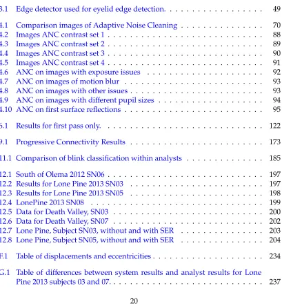
3.1 Edge detector used for eyelid edge detection. . . 49
4.1 Comparison images of Adaptive Noise Cleaning . . . 70
4.2 Images ANC contrast set 1 . . . 88
4.3 Images ANC contrast set 2 . . . 89
4.4 Images ANC contrast set 3 . . . 90
4.5 Images ANC contrast set 4 . . . 91
4.6 ANC on images with exposure issues . . . 92
4.7 ANC on images of motion blur . . . 93
4.8 ANC on images with other issues . . . 93
4.9 ANC on images with different pupil sizes . . . 94
4.10 ANC on first surface reflections . . . 95
6.1 Results for first pass only. . . 122
9.1 Progressive Connectivity Results . . . 173
11.1 Comparison of blink classification within analysts . . . 185
12.1 South of Olema 2012 SN06 . . . 197
12.2 Results for Lone Pine 2013 SN03 . . . 197
12.3 Results for Lone Pine 2013 SN05 . . . 198
12.4 LonePine 2013 SN08 . . . 199
12.5 Data for Death Valley, SN03 . . . 200
12.6 Data for Death Valley, SN07 . . . 202
12.7 Lone Pine, Subject SN03, without and with SER . . . 203
12.8 Lone Pine, Subject SN05, without and with SER . . . 204
F.1 Table of displacements and eccentricities. . . 234
G.1 Table of differences between system results and analyst results for Lone Pine 2013 subjects 03 and 07.. . . 237
[image:21.612.110.519.250.693.2]Introduction
Vision is part of complex human behavior and gaze is a precognitive indicator of a subject’s attention [2,3]. A subject’s fixation patterns indicate their cognitive strategies, but are not consciously available to a subject. Even though not cognisant of their actions, people use the world as an external storage for information [2]. In order to extract information from the world, people must look at the objects in the world and fixate the world on their retinas. The patterns that subjects use to access that information can reveal important insights into their problem solving strategies, even if the subject is not consciously aware of these strategies [3].
The process of determining where a person is looking in the world requires a recording of where the eye is looking, a frame of reference for the world around them, and a correspondence formed between the two. To form a correspondence between the pose of the eye and the location of attention in the scene, the first step is to determine the pose of the eye for every frame of recorded eye motion.
This eye pose, or pupil location, must be located regardless of other noise present in the scene, such as reflections, shadows across the eye, deep shadows of the corners of the eye, and partially occluded pupils by the eyelids.
Commercial fully-automated eye-tracking systems are available for processing indoor eye-tracking tasks. For outdoor eye-tracking the fully-automated system become unre-liable. To compensate for that unreliability a labor intensive, completely manual system was developed including custom software. An analyst used the software by looking at each frame and locating the pupil in each individual frame of the eye video. The fully-manual system allowed an analyst to process videos at a rate of two to three frames per minute.
A previous method for assisting in the coding of these videos was developed and patented [4]. This method was instantiated in a program namedSemantiCode[5]. Seman-tiCode was subsequently commercialized and licensed. While helpful, the program still requires that every frame in the input video have the eye location correctly identified it
starts.
This work provides analysts with a tool that automatically locates pupils quickly, even under challenging conditions. This work was developed to locate the pupil in videos of the eye that are captured under challenging conditions at a faster rate than manually labeling every single frame of the video.
The larger goal is to analyze observer behavior in natural outdoor conditions that include being surrounded by high contrast daylight, sudden changes in illumination, and first surface reflections offthe cornea of the eye [6,7].
1.1
Problem Statement
In a portable eye tracking study, a subject’s eye is followed with a head mounted camera. This records the subject’s eye pose throughout the study, which then requires that the subject’s pupil be located in every frame of the video.
This pupil location is then used with a calibration sequence to form a mapping from where the subject’s eye pose is in the eye video, to where the subject is looking in the real world (the scene).
Fully automated video based eye-tracking systems work for indoor tasks when the lighting is controlled and the user is constrained to a limited range of motion. Previous work at MVRL developed and used pupil detectors based on Loy and Zelinski’s fast radial circle detector [8], [9]. That approach worked well for indoor eye tracking, but when the pupil became elliptical the circle detector located an end of the pupil ellipse instead of the center of the pupil ellipse. Each end of an ellipse has a focal point, and circle detectors tend to find these.
Our goal is to analyze observer behavior in natural outdoor conditions that include being surrounded by high contrast daylight, sudden changes in illumination, and first surface reflections offthe cornea of the eye [6,7].
All of these issues arise when eye-tracking subjects are taken out of doors. Scientists are increasingly taking eye-tracking studies outside in uncontrolled lighting. Even when the eyes are shaded from direct sunlight using large hats, some of the previously listed issues still remain.
The Rochester Institute of Technology’s Multidisciplinary Vision Research Lab (MVRL), in collaboration with the University of Rochester, is involved in a multi-year NSF study tracking the eyes and gaze patterns of geology students and experts [6]. Since multiple students were eye-tracked for multiple hours over multiple days, and since the study was a multi-year study, a large amount of data is generated.
becomes intractable. Processing of these videos requires having analysts manually locate the pupil in every single frame of the video.
Using custom developed software an analyst can processes two to three frames per minute. Each analyst must be carefully trained, and the analyst is susceptible to fatigue from hours of sitting and inspecting video frames.
The goal in this work is to increase the data processing rate – the rate at which we can identify the center with certainty the pupil location in a video of a subject’s eye as they are being eye-tracked.
The end result is the location of the center of the pupil in each frame, which is subsequently used to discover where the subject was looking in the scene.
The rest of this chapter discusses some of the challenges we faced in trying to reduce the amount of human-computer interaction while still maintaining pupil location accurately.
1.1.1 System Requirements
Mobile eye tracking uses two head-mounted video cameras on human subjects to record:
• the position of the subject’s eye in their head (recorded in the “eye video”), and • the scene in front of the subject (recorded in the “scene video”).
These videos are recorded continuously throughout the study.
These two videos (eye and scene) must be kept synchronized for later calibration. The latest capture system synchronizes these eye and scene frames automatically.
1.1.2 Calibration
During data collection, we ask the subjects to look at known points in the scene and move their heads in fixed incremental amounts. In this way their gaze traverses the full range of eye motion. The points from this calibration sequence are then used to provide the points required to form a calibration.
By forming a correspondence between the two videos we are able to estimate where the subject was looking in the scene at every point in time with the temporal resolution limited by the frame rate of the video.
The correspondence between the location of the eye-in-head to the location of the gaze-in-world can only be formed if the location of the pupil in the eye is correctly identified in every frame of the video of the eye.
1.1.3 Mobile Eye Tracking Requirements
For indoor eye tracking where the illumination is stable, and when the light incident on the cornea of the eye is controlled by a voltage regulator, eye-tracking is a solved problem. One can purchase or make an eye tracker that correctly tracks the pupil location [10–12]. One requirement for commercial eye trackers is that the lighting (illumination) is controlled. This requirement breaks down in many situations, such as:
1. when the subject walks up to a window,
2. if there are moving lights in the scene surrounding the eye (such as when driving), or
3. if the subject goes outdoors in bright sunlight.
Bright sunlight is problematic outdoors even if the subject is wearing a large hat to shade their face, because as the subject’s head rotates from facing towards the sun to looking away from the sun the amount of light reflected onto the face can change by several orders of magnitude.
The autoexposure algorithm in the video camera attempts to compensate for changes in the amount of light, but this algorithm always lags the changes. Furthermore, as the camera’s exposure algorithm adjusts the exposure it also adjusts gain and contrast controls which in turn changes the global histogram for the entire image of the eye on a frame-by-frame basis.
Unfortunately, the system records no meta-data about how much contrast or exposure compensation was applied. We cannot invert the contrast adjustment or the exposure compensation that was applied to each frame.
1.2
Data Inundation Problems and Issues
The most common technique these days for eye-tracking is video-based recording of the eye motions [13]. Yet, this advancement in the ability to record the data leads to all the issues associated with large amounts of data.
The study becomes inundated with data and must use data reduction techniques to reduce the data to a manageable amount.
The following subsections discuss some of these issues, and the need to efficiently process data.
1.2.1 Data Inundation in Frames
patterns of geology students and experts. During this study 12 subjects are eye tracked for about 2 hours a day, over 10 days (2011) [6]. The trip returns with roughly half a terabyte of data to analyze.
Over the course of the ten days, the number of video frames collected can be estimated by making some rough assumptions:
• 2 videos per subject,
• times 29.97 frames per second per video, • times 60 seconds per minute,
• times 60 minutes per hour, • times 2 hours per day,
• times 12 subjects tracked per day, • times 10 days of tracking
The product of these factors is about 5.2x10⁷ video frames each year. The study spans multiple years, so the maximum number of video frames is potentially higher.
1.2.2 Data Inundation in Pixels
Section1.2.1discussed the number of frames that must be analyzed by a human looking at each frame of the eye video. Here we consider this number of frames in terms of data. If each frame was only 240 rows and 320 columns and monochrome, that would be 76,800 pixels per frame. In terms of uncompressed data, for the 26 million frames, this amounts to 3.7 terabytes of data that must be processed for the eye videos alone.
This is a tremendous amount of data to contend with, both from the point of view of the analyst looking at the videos, and from the point of view of a computer that must read, process, and annotate the data.
1.2.3 Yarbus Software
In our eye tracking work flow, the process of locating the subject’s eye in every video of the eye is usually handled by the Positive Science®eye-tracking software called Yarbus®. This software works well for standard, uniform, office lighting situations. However, it breaks down when the subject takes the mobile eye-tracking headgear outside.
• The subject goes outdoors, where the illumination on the eye is not controlled only by the illumination from the Positive Science®eye tracker. Generally, an infrared LED (IRED) is used by the eye tracker to illuminate the eye. A subsequent section will compute the amount of illumination caused by reflected background lighting when eye tracking outdoors in bright sunlight (See AppendixC).
• The illumination of the eye changes quickly, as when the subject rotates his/her head quickly, or when driving in dim light in the face of on-coming car headlights.
• The subject’s eyelashes go in front of the pupil. Eyelashes in front of the pupil change the local photometric value of that region of the image, and occlude the features of the pupil. The local pixel values become either lighter or darker.
1.2.4 Data Reduction Techniques for Analysis
While each observer might be eye tracked for two hours per day, it is often the case that a few critical minutes of the video data can be identified as most important to process. Once the critical data has been identified, those sections of eye-and-scene video data are the only sections that need to have the eye movements and fixations precisely analyzed. The analyst’s job is simplified by first identifying and isolating these sections of the eye tracking videos.
The identification of the sequences of interest is one method of data reduction. Typ-ically for each subject the critical frames include a sequence that is used for calibration, and another sequence during which the subject is asked to do a visual search or visual analysis of the scene.
As another data reduction technique, the subject’s fixations are computed. These fixations are the times at which the eye is stable with respect to the world. At these times the image of the world around the subject is stable on the retina. However, fixation analysis cannot take place until the pupil is located in each frame.
The data reduction techniques mentioned here are procedural techniques, used by analysts processing the video to reduce the number of frames that need to be processed. Other techniques are used in the algorithms to reduce the amount of memory necessary.
1.2.5 Pupil Location
Before calibration can occur the pupil center must be located in the eye video.
However, current pupil location systems fail when used under challenging lighting conditions, which occur as soon as the subject steps up to a bright window.
In such situations, the standard assumptions fail. For example, the pupil is not the darkest location in the eye image, the corners of the eyes are. As a result, pupil location techniques that use only the pixel value fail.
Other techniques do not use the pixel value itself, but the relative pixel value in the region. An easy example to consider is the locally darker edges that indicate a pupil. However, edges themselves are unreliable because edges detected in the eye video are not always caused by the eye itself. Edges can be caused by the world being reflected off of the cornea of eye.
The current work-flow for locating pupils in each frame of a subject that has been outside involves having students step through the video frame-by-frame, using custom software, and identify the pupil location and size in each frame.
Analysts can do this task because the human visual system (HVS) automatically performs background subtraction. A trained human vision system automatically ignores things that are not relevant to the task. This top-down aspect to the HVS lets us ignore skin surrounding the eyes, sclera (white of the eyes), eyebrows, the corners of the eyes, eyelids, eyelashes, stray hairs in front of the camera, and reflections offof the eye.
In this thesis we will mimic several of these aspects of the HVS in order to better recognize and fit the pupil locations. We draw inspiration from how the human vision system works. The intention is to use computer analysis to increase processing through-put, decrease uncertainty in the data, and reduce the data analysis effort specifically for natural outdoor images.
1.3
Processing Stages
1.3.1 Automated Approach
From the start, it was known that detecting the pupils of subjects under these circum-stances would be difficult.
The initial design was to use several passes over the video streams to capture the pupils. The idea was to have an early pass identify the most reliable and stable pupils automatically. The knowledge of where these reliable pupils were would be used to learn the parameters of the subject’s motion, and bootstrap the detection of the rest of the pupils in a subsequent pass. As a final pass, the user would validate the pupils.
The original sequence of processing steps included:
1. Statistical collection on all frames, to identify stable pupils for detection.
3. Parameter learning of the subject’s range of eye motion, and variations across the video sequence.
4. Subsequent processing of the frames to identify the less stable pupils.
5. Final user validation of the pupils.
This was implemented, and shown to work for several subjects. Unfortunately subject-to-subject variations caused the automated methods to work for some subjects but fail for others.
Since the subject-to-subject variations were too large for a fully automated solution to work reliably on all subjects, a method to determine the pertinent parameters for each subject was needed. We achieved this through the use of semi-supervised feedback.
1.3.2 Use of Semi-Supervised Learning
To collect ground truth data from the first pupil detection stage, a validation pass was created. This validation allowed the initial set of pupils to be used as ground truth for discovering the parameters and range of variation for subsequent pupil detection.
The decision to validate the first set of pupils was pivotal in getting the program to work reliably for multiple subjects. The pupils from the most stable frames provided subject-specific information about the changes in edge strength, pupil darkness, sur-rounding iris brightness, as well as the angle of rotation and eccentricity of the pupil ellipses as a function of position in the image.
Using the validated ground-truth pupils from the first pass, the parameters of the eye model could be found independently instead of using an optimization method to try to solve for both simultaneously. The availability of this ground truth also provided several opportunities for machine learning and parameter modeling.
Figure1.1shows the main stages for identifying the pupil. These stages involve:
1. Statistical collection on all frames. These statistics are used to identify stable pupils for detection. The stable frames serve as a sampling of the full video, in such a way as to avoid closed eyes and eyes in motion.
2. An initial pupil detection on these most stable frames. This identifies the most likely pupil locations in each of these frames.
3. Validation of these detected pupils. The user checks the located pupils to assure that they were located correctly.
5. Final user validation of the pupils. In this phase the user has the chance to examine all of the detected pupil position.
Collect statistics on all frames.
User validation of initial pupil fits.
Sample initial pupil frames to determine
system modeling parameters.
Model generation for subject followed by
exhaustive pupil detection in all frames.
Final user review and validation.
Input video
Pupil positions
Figure 1.1: The main stages of processing for pupil location.
1.4
Innovations
The core routine used to identify and locate the pupil is a circular Hough Transform, a circle detector. The Hough Transform was optimized for pupil detection as described in Ch.5.
However, the Hough Transform relies on correctly detecting the pupil-to-iris edges. Especially when trying to detect small pupils, it is thrown off by other edges in the image. Any techniques that can remove non pupil-to-iris edges improve the accuracy and detection rate for the Hough Transform.
To improve the reliability of the Hough Transform, noise cleaning and image smooth-ing are used. This noise cleansmooth-ing includes removsmooth-ing the eyelids around the eye, ussmooth-ing a similar technique similar to that of Masek [14]. The details of eyelid removal are described in Ch.3.
The presence of other edges that reflect offthe first surface of the cornea of the eye cause additional false positives in the Hough detector. Noise from compression artifacts is also an issue in these images. To remove this noise an adaptive noise removal technique was developed which takes advantage of the structure of the eye.
This pixel-by-pixel noise cleaning technique involves an edge-preserving noise smooth-ing algorithm, based on Kuwahara’s work [15]. The developed algorithm is several times faster than a bilateral filter, and has one quarter the false alarms as the bilateral filter. This process is described in Ch.4.
The initially detected pupils are used to develop a model of the subject’s eye. This model is used to apply a non-linear subject-specific transformation to the eye image which converts elliptical pupils into circles. This technique, called unwrapping the eye, is described in Ch.6.
That same model of the subject’s eye allows the program to identify pupil ellipses that would never occur on a real human, and automatically reject them. Some pupil ellipses are tilted the wrong way, and could not possibly be correct pupil detections of the subject’s eye. Using the model, thesestrange ellipsescan be identified and rejected in a process called strange ellipse rejection, as described in Ch.7. Strange ellipse rejection improves the accuracy and reliability of the entire program.
Using multiple features creates a higher dimensional space for analysis. The benefit for this is that the data becomes sparse. This sparsity can be taken advantage of by isolating the target points in feature space. The method for feature combination is described in Ch.8.
Once the pupil location has been detected, an adaptive edge following scheme is used to follow the contours of the pupil. This technique, called progressive connectivity, is described in Ch.9.
the degree of confidence is used to sort the highest confidence pupils to the first position in the list of possible pupils. The degree of confidence is described in Ch.10.
Workflow and Primary Passes
This chapter provides a high level overview of the primary passes used to locate and detect pupils in the eye videos.
Figure2.1shows a block diagram of the main stages, or passes, of the work flow. Each of these passes are described in the following sections.
Figure 2.1: Overview of main processing and workflow.
2.1
Overview of Primary Processing Passes
When asked to find pupils in a frame of a video, a natural question is, “Why don’t you just use a circle detector?”
Circle detectors work very well in situations when the images are of coins taken on axis of the coin, with a simple contrasting background. Such images exist in assembly lines where the lighting is controlled and the background is a uniform contrasting color designed to simplify the computer vision task.
The program makes several passes over the data. In each pass select video frames are read in, examined, and processed. Not every frame of the video is read during every pass.
The following passes are used to locate the pupil in the frames of the eye video:
1. Statistical collection pass.
An initial statistics collection pass to detect sudden changes (such as blinks) and regions of the video frame that can be ignored throughout the entire video.
2. Sampling pass
An initial easy-pass samples the video frames that are likely to contain strong circular pupils without motion blur. This easy-pass includes masking offinvariant pixels (Section2.2.1), eyelid detection (Chapter3), circle detection (Chapter5), and edge refinement (Chapter9). The result is an initial guess at the pupil locations for approximately301 of the frames in the video.
The Hough detector for this pass is fast and not as complicated as later stages. Pupils that are highly eccentric because the eye is looking away from the camera are missed. The expectation here is that the frames analyzed will be stable, with little motion, and the pupils will be close to on-axis.
3. User validation pass
The user confirms or fixes the pupils detected in step 2. User validation creates known ground truth frames that the program can then build models from.
4. Pupil edge modeling
The pupils that were confirmed to be valid are used to form models of the edge strength as a function of position.
5. Geometric modeling
The program uses information from the pupils found previously to determine the eye size and center of rotation. A geometric model of the subject’s eye results. This determines how to unwrap the eye image so that the elliptical pupils in the eye image become more circular. Unwrapping is a non-linear image transformation that converts eccentric pupils into more circular pupils that can be detected by the circle detector.
6. Automatic pupil detection pass
7. Final user validation
A final user-validation pass over the pupils allows the user to inspect and select from the program’s three candidate pupils. The three candidate pupils can be selected by the analyst with the push of a single button. The analyst can also refine the pupil location by manually clicking on five or more edge points around the pupil edge. A pupil ellipse is then fit through those points.
2.2
First Pass and Statistical Collection
The first pass over the data collects statistics about the frames of the video being processed. These statistics are used for several three reasons: 1. background removal, 2. blink detection, and 3. stable frame identification.
2.2.1 Background Removal Statistics
During the first pass, two important statistics are collected over the entire video range specified. The first is an average frame over frames of the video being processed. This is an average value for every single pixel in that range of frames. The second statistic is the standard deviation of each pixel over that same range.
Pixels that have very low standard deviation are ignored. Pixels that do not change over the course of the video cannot contain information relevant to this task.
1 foreach framedo
2 //Find the center region of the image, which gives the best signal: ;
3 Vvt=vector of center half of vertical pixels ;
4 Vhz=vector of middle 5/7 of horizontal pixels ; 5 Cf rame= f rame(Vvt,Vhz) ;
6 //Find the average and std of the center of the image itself: ;
7 Aif rame=mean(Cf rame) ;
8 Sif rame=std(Cf rame) ;
9 //Find the magnitude of spatial edge differences: ; 10 Espatial=abs(sobel edges) ;
11 //Find the temporal image difference: ; 12 Etime=Af rame(k)−Af rame(k−1) ;
13 //Record the statistics on the edge strengths: ; 14 Aespatial=mean(Espatial) ;
15 Aetime =mean(Etime) ; 16 Sespatial=std(Espatial) ;
17 Setime=std(Etime) ;
18 //Compute histogram of these temporal differences: ; 19 Htime=Histogram(Etime ) ;
20 //Find the absolute value of the change in the histogram: ; 21 Hchange=sum(abs(Htime(k)−Htime(k−1))) ;
22 end
Figure 2.2: Computing statistics for frames in first pass
2.2.2 Blink Detection Statistics and Algorithm
During the same first pass, frame-by-frame statistics are collected. These statistics are used to predict which frames are blinks, and to find frames that are very stable.
During the blink of an eye, the closing of the eyelid causes the global brightness of the video frame to change suddenly. Eyelids are brighter than the pupil. When the eye is closed the eyelid hides the crevices, pupil, and shadows of the open eye from the view of the camera. When the eye is closed, the video frame contains fewer edges. The statistics collected to detect blinks are all measures related to the image brightness and the number and strength of the edges present.
Figure2.2 gives the algorithm used to collect per-frame statistics. Spatial edges are computed, and statistics are collected on them. A temporal edge feature is also computed by computing a frame-to-frame difference, and statistics are computed on that.
The following per-frame processing is performed, and the resulting per-frame statistics are recorded.
Figure2.3gives the algorithm for blink detection. The frame brightnesses are normal-ized to a range of [0,1], so that video-to-video changes can still use the same algorithm. This normalization also compensates for exposure condition. The intuition here is that a frame is a blink if it is more than 0.20 above the running average over 15 frames. This means that the frame is suddenly much brighter than the local average. If the frame is in the top 70% of the brightness range, then it is probably a blink as well.
1 //Find the min and max brightnesses from average frame illumination: ; 2 Bmin =min(Aif rame(:)) ;
3 Bmax=max(Aif rame(:)) ;
4 //Compute the normalized brightnesses. Values are in range [0,1]: ; 5 Bnorm=(Aif rame(:)−Bmin)/(Bmax−Bmin) ;
6 //Compute running avg over 15 frames: (half second) ;
7 Bavg=sum(Bnorm(k−7,k+7))/15 ;
8 //Classify blinks: ;
9 Blink=(Bnorm−Bavg)>0.20 ∪ (Bnorm>0.70) ;
Figure 2.3: Classifying blink frames
2.2.3 Stable Frame Identification
Along with the differences from the frames, the data that is collected is used to identify the most stable frames. The first pass uses thesemost stable framesas the best frames to try to detect pupils in because they are least likely to have fast eye motions.
The statistics from the initial pass (see Figure2.2) are used to derive a measure of how much a frame differs from the norm for the video. We assume a multivariate Gaussian distribution for these variables, perform principal components analysis (PCA), and use the resulting eigenvectors as input to a Karhunen-Lo`eve Transform (KLT) [16, p. 266] The KLT subtracts offthe mean values and rotates the data to axially align it. The Mahalanobis distance from the norm is then computed [16, p. 25].
The result is a distance from the norm for every frame. This distance from the norm is used in the following passes to identify pupils that are most likely to contain an open eye. The more normal the frame is, the more stable it is.
2.3
Easy-Pupil Detection Pass
Once the stable frames have been identified, they are analyzed to find the initial pupils. This easy-pass examines only a sample of the frames to identify likely strong circular pupils. Figure2.4diagrams the processing used during this pass.
The statistics collected are used to form a mask for removing pixels from consideration. The pixels with the lowest standard deviations are used to establish a mask of pixels that do not change throughout the video. This is called aninvariant pixel mask. This mask is constant throughout and is used for every frame of the video.
In addition to the invariant pixel mask, an eyelid detector is used to find the upper and lower eyelids, as described in Chapter3. The regions above the upper eyelid and below the lower eyelid are masked offand ignored.
Adaptive noise cleaning is used to remove edges that do not match the model of structured edges for pupils, described in Chapter4.
All of this pre-processing is done to reduce the amount of work needed for the Hough circle detector, described in Chapter5. The Hough circle detector for this pass is faster and not as complicated as later stages. It does not try to compensate for elliptical pupils. Pupils that are highly eccentric because the eye is looking away from the camera are missed. The expectation for the easy-pass is that the frames analyzed will be stable, with little motion, and that the pupils will not be far offaxis.
An edge refinement and contour following scheme is used to refine the pupils detected, as described in Chapter9.
From this the candidate pupils detected in each frame are ranked, based on a degree of confidence metric, as described in Chapter10. The top three candidate pupils, with the highest degree of confidence are retained for consideration by the user.
Figure 2.4: Processing in the easy pupil detection pass.
2.4
First User Validation Pass
Given the pupils from the initial pass, the user can then inspect the pupils found to assure that they are correct. The result of this validation is labeledground truthpupils.
The initial goal of this pass was to find the good pupils to use for building the geometric models of the eye.
Figure 2.5: Diagram of the user validation pass, showing that it creates known correct and incorrect pupils.
2.4.1 Establishing Ground Truth Pupils
Each pupil has a degree of confidence (DOC) associated with it. The user can set a threshold for the range of DOC he or she is interested in. Because of this, pupils with a very high DOC can be automatically ignored and not examined. The user can elect to examine only those frames for which the pupils have a very low DOC.
During this first validation pass the top three pupils for each frame are presented to the user. The user can then select from these top three with the push of a single button. The user can also refine the pupil location to get a more accurate ellipse for the pupil position. Alternatively, the user could reclassify the frame as a blink.
2.4.2 Establishing GroundFalsePupils
There is another benefit of this first user validation that was not initially obvious – it establishes knownbadpupils.
Each stable frame that was analyzed retains the top three candidates for pupils that were found. Since only one of them was selected by the validation pass, the others two candidates are known to be wrong. The user validation pass establishes both correct and incorrect pupil locations. Itlabelsthe candidate pupils as being good or bad. This provides the data needed for a two class classification problem, one class is known to be good, and the other class is known to be bad.
When the process of validating the pupils from the easy-pass was started, it was not obvious that by notselecting the wrong pupils the incorrect class of pupils was being labeled implicitly.
Using the set of candidate pupils that were rejected, we convert the problem from only matching the best pupils, into the task of matching the best pupils and simultaneously avoiding the wrong pupils. This knowledge is used to automatically reject pupils that are the wrong size for their location in the frame, or that are rotated incorrectly for pupils in the eye frame. These pupils that can be identified as the wrong size or the wrong rotation are termedstrangepupils. The process of strange pupil rejection is described in Chapter7.
2.5
Modeling
2.5.1 Edge Strength Modeling
Once the edges of the ground truth pupils are identified, the minimum and maximum edge strengths can be modeled. The ground truth pupil locations provide known pupil edge locations, and from these the minimum and maximum edge strengths can be ex-tracted for each position, across all the video frames that contain the ground truth infor-mation. Using these known minima and and maxima, maps are created for the weakest and strongest edges within 100 pixels of any location in the frame.
The resulting edge strength maps are used in the automatic pass, to automatically remove edges that too weak or too strong to be associated with a pupil.
This automatically removes some edges, such as those caused by the subject wearing glasses, because the edges are too weak to be pupil edges. The edge strength models are also used to remove edges that are too strong, such as those caused by strong first surface reflections offof the cornea.
2.5.2 Eye Geometry Modeling
Chapter6.
The two key parameters for the model is the (x,y) location of the center of rotation of the subject’s eye in the video frame, and the approximate size of the subject’s eye. These parameters are derived from the ground truth pupils collected from the first user validation pass.
2.6
Automatic Pupil Detection Pass
A block diagram of the automatic pupil pass is shown in Figure2.6.
Once the parameters of the eye have been discovered, this second pass over the video is used to fill in the pupils for frames that were not previously analyzed.
The first pupil detection pass samples only one 1 of 30 pupil frames, or roughly one frame per second. This automatic pass is responsible for finding pupils in 29 out of 30 frames, or approximately 97% of the frames.
Since most of the frames are analyzed by this automatic pass, extra steps are used to try to assure robust automatic processing. This pass takes advantage of the previous models of the subject’s eye geometry, and the parameters that are used to identify and automatically rejectstrange pupil ellipses.
As with the easy-pass, this pass uses adaptive noise cleaning, and contour following to refine the pupil edges. Candidate pupil ellipses found are assigned a degree of confidence (DOC) measure.
However, before the pupil is located using a circle detector, the image of the eye is first unwrapped. A Hough circle detector is then used to locate the pupil in the unwrapped image. Because of the importance of this automatic pass, the Hough circle used modified to allow it to detect more eccentric circles in addition to nearly circular pupils. This adds an additional second per frame for detection, and adds additional false positives, but assures that the pupil is not missed.
Figure 2.6: Block diagram of the automatic pupil detection pass.
2.7
Final Inspection
After any pass, the user can inspect and modify the pupils located. This task is very similar to the routine for user verification described in Section 2.4. For the user, this inspection is the majority of the work. The previous pass over the data automatically identified three pupil candidates in every frame. The goal of that work was to locate the pupil correctly. In this final inspection, the user is responsible for verifying that the correct pupil of the three was selected automatically. If the program selects the correct pupil as one of the top three candidates, then the user can hit a button to select it automatically, and proceed to the next frame.
Alternatively, if the program found three incorrect pupil candidates, the user can manually identify the pupil by entering at least five points on the border of the pupil. Using these points, the program fits the pupil ellipse.
2.8
Summary
The initial pass collects statistics that are used to guide the rest of the processing passes, and to ignore pixels in the video which do not change over the course of the video.
The initial statistics are also used to identify frames that have little frame-to-frame change, the frames that are deemedmost stable.
An initial easy-pass examines thesemost stableframes to find pupil candidates. These frames constitute about three percent of the frames in the video. The processing used for the initial pass is simpler, and more error prone, than the final automatic pass because it does not know the eye geometry of the subject. The user must inspect the output of this easy-pass, and correct any mistakes.
The frames that result from validating the results of the easy-pass are used to build subsequent models of the eye geometry, and to establish the limits for the maximum and minimum pupil edge strengths as a function of pixel location throughout the entire video. The automatic pass then analyzes the remaining 97 percent of the video frames, using those models. This automatic pass includes a non-linear geometric transformation that converts the ellipse of the pupil into a circle so that a circle detector can be used to find the pupil ellipse. This operation avoids the need to use a complicated ellipse detector. Compared to an ellipse detector, the circle detector uses less memory and greatly reduces the number of parameter combinations that must be considered.
Eyelid Location and Removal
3.1
Overview
In this chapter we describe the process of finding the eyelids and removing the uninter-esting image regions from consideration by the pupil detector. These regions include the image above the top eyelid and below the bottom eyelid.
Regions outside of the two detected eyelids are masked off, and removed from con-sideration by the pupil detector.
Figure3.1 shows an example of the eyelid detection and masking results. With the upper and lower eyelids detected, a mask is formed to remove pixels above the upper eyelid and below the lower eyelids. This removes additional eyebrow hairs and eyelashes that could be a distraction for the Hough circle detector.
(a) Input Frame (b) Detected Eyelids
Figure 3.1: An example showing the upper and lower eyelids that were detected. The cyan and red lines on the left of Figure3.1(b)show the inter-mediary calculations used to find the eyelids. The cyan and red horizontal lines are the rows of the lower and upper eyelids that were detected.
Removing the region of the image outside of the eyelids has two benefits. First, it removes sections of the image that include eyebrows, and eyelashes, and thus reduces regions of the image that could cause false alarms when looking for pupils. Second, it reduces the amount of the image that needs to be processed by the downstream processing. We use an eyelid detection approach inspired by Masek’s description [14], but de-veloped independently, to accommodate the fact that our subject’s eyes are not always opened. Masek had cooperative subjects, who held their eyes open and steady so that they could be recognized by the iris recognition system. We have subjects whose eyes are in motion, ideally not thinking about the fact that their eyes are being imaged, and whose eyes are often squinting in bright light and are sometimes closed during blinks.
It is important that the process be conservative so that it does not err on the side of accidentally masking offa region where the pupil could be located.
The approach consists of an edge detector, histogram projection, lower eyelid detec-tion, upper eyelid detecdetec-tion, and use of some conservative association rules.
We cannot assume that the eye will be fully opened, and that the lower eyelid will be concave upwards. In situations where the light is bright outside, subjects squint their eyes. In situations where the camera is located below a subject’s eye, the camera is looking up at the eye and the lower eyelid is concave downwards.
3.2
Edge Detection for Eyelid Location
For the purposes of eyelid detection, we seek to detect a relatively large edge transition from dark-to-light or from light-to-dark.
The shadows that form between the eyelids and the surface of the eye are used to detect the eyelid.
We use a 5×5 edge detector. Table3.1gives the filter coefficients used for detecting edges for eyelids. The coefficients shown are used to detect horizontal edges, and the transpose of this table is used to detect vertical edges. The edge detector shown in Table3.1computes two local averages over five horizontal rows. One of these averages is two pixels above the center pixel, and the other is two pixels below a central pixel. The difference of these two averages is used to estimate the local image gradient.
For this application, the images are roughly 320 pixels wide, and 240 pixels high. Since the eyelids in these images are relatively large, the standard Sobel edge detector provides edge detection on too small a scale for this application. Instead, a different edge detector is used to detect the edges of eyelids. This edge detector was developed to emphasize larger transitions between objects.
The usual Sobel edge detector is only a 3×3 detector. It finds skin wrinkles, eyelashes, and the MJPEG (image compression) block artifacts that occur in the image. These edges are distractions from the true eyelid edges we hope to isolate and remove.
This wider filter has stronger support for edge detection because it is computed over a larger region. This means that it is less likely to detect small edges (such as MJPEG artifacts). The edges we seek are the large edges of the eyelids. For a fixed image gradient (such as a ramp) the image will change more over the longer distance of the five pixels than the three pixel Sobel edge detector. The 5×5 filter is working on a stronger input signal than a Sobel edge detector would be. The larger filter is more likely to detect the eyelid-to-eye transition, while being less sensitive to changes that occur over only a few pixels.
Using a larger filter is sufficient for detecting these edges, at the cost of decreased edge localization. In terms of localization, the 5×5 filter results in a step response over four pixels while a Sobel edge filter gives a step response over only two pixels. So the edges detected are less specific to a given area.
Table 3.1: Edge detector used for eyelid edge detection.
0.1117 0.2365 0.3036 0.2365 0.1117
0 0 0 0 0
0 0 0 0 0
0 0 0 0 0
-0.1117 -0.2365 -0.3036 -0.2365 -0.1117
Edges are detected both horizontally and vertically, and the magnitude and angle of these edges is estimated for the pixels in the center half of the input image.
Weak edges that have almost no edge strength and can occur in almost any direction. To compensate, only edges whose magnitude is in the top quartile are used for further computa


![Figure 6(a) from, Learning to traverse image manifolds, by Piotr Doll`aar, et. al. [80], from](https://thumb-us.123doks.com/thumbv2/123dok_us/94376.8874/124.612.152.457.355.586/figure-learning-traverse-image-manifolds-piotr-doll-aar.webp)