Encoding Possible Final States of the Universe with Conformal Structures

(1)

Encoding Possible Final States

of the Universe

with Conformal Structures

By

Philipp Andres H¨ohn

November 3, 2006

A thesis submitted for the degree of

Bachelor of Science with Honours in Theoretical Physics

at the Department of Physics

Faculty of Science

(2)

(3)

Declaration

I certify that the work contained in this thesis is my own original research, produced in collaboration with my supervisor – Dr. Susan M. Scott. All material taken from other references is explicitly acknowledged as such. I also certify that the work contained in this thesis has not been submitted for any other degree.

Philipp H¨ohn

(4)

(5)

Acknowledgements

I’d first like to thank my supervisor Dr. Susan Scott who has had most influence. Thank you Susan for offering me this wonderful opportunity of researching my Honours thesis under your supervision and for leaving me the freedom to pursue my own ideas freely. The discussions with you have provided me with optimal guidance and inspiration for my investigations. Thank you also for the patience you have shown when proof-reading sections of this thesis. You have been an instructive mentor and I greatly appreciate how you have looked after my academic well-being. I would also like to thank my office mate Dr. Mike Ashley whose LA_{TEX and} computer expertise has saved valuable time for the physics in this thesis. Thanks also for the valuable discussions about General Relativity and the structure of space-time. Sharing an office with you Mike has undoubtedly made a difference to this thesis and added memorable personal experiences to my year in Australia.

For proof-reading some technical results and patiently discussing some of my calculations with me I’d like to thank Ben Whale, whose further suggestions have been useful to this research.

Finally, but by no means least, I would like to express my gratitude to the Deutscher Akademischer Austausch Dienst (German Academic Exchange Service) for the scholarship which I was awarded. This research would not have been possible for me without this financial support.

Philipp H¨ohn Canberra November 2006

(6)

Abstract

The concept of an Isotropic (Past) Singularity (IPS) was defined by Goode and Wainwright in 1985 as a mathematical formalisation of quiescent cosmology and the Weyl Curvature Hypothesis (WCH) for the isotropic initial state of the universe.

In this thesis it is argued that the framework of an IPS is not sufficient to guar-antee a future behaviour which is compatible with the future anisotropy implied by quiescent cosmology and the WCH. Therefore it is necessary to complete and com-bine the framework of an IPS with new definitions, in order to assure an appropriate past and future behaviour of a cosmology satisfying the respective combination of definitions. Since it is not yet clear whether our universe will expand indefinitely or recontract, it is reasonable to provide a new definition for the scenario of an ever expanding cosmos and one for a recollapsing universe.

Specific example space-times are explored for their conformal structure, future evolution and compatibility with the WCH as guidance in the quest for the new definitions. Motivated by these particular models, we present for the first time the definitions for the conformal structure of an Anisotropic Future Endless Uni-verse (AFEU) and an Anisotropic Future Singularity (AFS). For the purpose of completeness and comparison, we furthermore define the physically less realistic

Isotropic Future Singularity (IFS) and the Future Isotropic Universe (FIU).

A number of essential technical implications of the new definitions are derived. It is explicitly shown that a conformal structure, whose conformal factor is a function of cosmic time, necessarily leads to an asymptotically Ricci dominated Weyl curva-ture and asymptotically expansion dominated kinematics, if the conformal metric remains regular. This condition is satisfied by the IFS and FIU. Based on this, it is argued that a conformal structure for an anisotropic final state of the universe requires a degenerate conformal metric, as is the case for the AFS and AFEU.

This degeneracy complicates the derivation of physical attributes of the concepts of an AFEU and an AFS and, consequently, new approaches are unavoidable. Some physical properties are examined, such as the behaviour of the expansion scalar and the curvature. It is proven that the conformal space-times always possess a future singularity, which under reasonable assumptions corresponds to a strong curvature singularity. Finally, we reveal sufficient conditions for the AFS, as well as the IPS, to be a strong curvature singularity.

The combination of the IPS with the AFEU and the AFS could provide a possible first version of a complete mathematical formalisation of quiescent cosmology.

(7)

Introduction

It was not until 1917, with the submission of the paper “Kosmologische Betra-chtungen zur Allgemeinen Relativit¨atstheorie” (Cosmological Considerations in the Theory of General Relativity) by Einstein [1] to thePreussische Akademie der Wis-senschaften (Prussian Academy of Sciences) in Berlin, that cosmology came into being as a quantitative natural science. Its aim is to determine the evolution and large-scale structure of the physical universe.

The problem of mathematically formulating cosmological models which might appropriately describe the universe has been a rather controversial story. Due to the lack of known evidence about the evolution of the universe, there have been many different viewpoints on what features these models should possess. Most of the models are based on the Theory of General Relativity, while rather recent models arise from Quantum Gravity, Quantum Cosmology and String Theory. Elementary particle physics has also proven to be essential for the understanding of the evolution of the universe; it has contributed significant ideas to cosmology, such as inflation and other concepts for initial conditions. An understanding of cosmology requires the merging of the physics of both the microcosm and the macrocosm.

Gravity is the dominant force on cosmological scales. General Relativity has turned out to be, so far, the most reliable theory for gravitational interaction on scales of the solar system and we shall assume in this thesis that this is also the case for scales of clusters of galaxies and the universe itself. Therefore this work will be based on the Theory of General Relativity and thus here the energy content of the universe will determine our space-time’s geometry. Matter and radiation contribution to the energy content can be described in several ways; here we will adopt Einstein’s idea of treating it as a fluid.

The focus of this work will lie partially on the very beginning, but mostly on the final state of the universe. By studying initial and final singularities we will explore the limits of this theory. These limits need not be the end of the physical world, however, and we will leave it open for a more precise and appropriate theory of gravitational interaction to extend (or perhaps replace) the view gained under the assumption of the validity of General Relativity. Quantum Gravity or String Theory might be possible candidates for this task.

The vast majority of cosmological models are based on the philosophical view-point known as the Copernican Principle. It states that “we do not occupy a

(12)

2 1. Introduction

ileged position in space-time”. This implies that local physical laws are the same everywhere in the universe and, furthermore, that our view of the universe is not a preferred one, when it comes to astronomical observations. This is a reasonable and greatly simplifying assumption.

A further assumption often used in cosmology, justified by observations, is

isotropy, which in the cosmological context simply means that large-scale obser-vations and effects are direction-independent. Belief in the Copernican Principle

then leads us to assume that this isotropy must be seen from every point in space-time. Homogeneity is another simplifying assumption which, in cosmology, means that physical conditions are the same everywhere in the universe and also that the metric we use to measure distances is valid everywhere in space-time. This, of course, is just an application of the Copernican Principle.

Einstein’s first model was based on an infinite, homogeneous and isotropic uni-verse without boundary for which he needed to introduce the cosmological constant Λ in order to enforce a constant size of the universe. In 1922, however, Friedmann published a work which showed that this constant was unnecessary if one would accept a time dependent length-scale of the universe. This work became significant after the discovery of the red-shift of galaxies by Hubble in 1929, which indicated that the universe is expanding.

There are a number of models which describe an isotropic universe. The astro-physical community most commonly uses theFriedmann-Robertson-Walker (FRW) family of models which we will briefly introduce in chapter 3. These models treat the universe as an isotropic, homogeneous, maximally symmetric and irrotational per-fect fluid without shear and acceleration, but with non-vanishing expansion. They combine the metric of Robertson and Walker with the Friedmann equations which are solutions to Einstein’s field equations. In fact, it can be shown by using mea-surements of the Hubble factor, that if the FRW models would describe the actual universe, then it must have originated from a singular initial state - a hot singularity at which energy density, pressure and space-time curvature were divergent - thebig bang.

In 1948 Gamov et al. predicted the cosmic microwave background (CMB) as a remnant radiation of the hot beginning of the universe. It was only in 1965 that Penzias and Wilson discovered this radiation by chance and the community immediately interpreted it as having originated in the big bang. From observations of the CMB via the satellites COBE (Cosmic Background Explorer) and WMAP (Wilkinson Microwave Anisotropy Probe) and of the matter distribution in our observable vicinity, it is well known that the universe is, in fact, extremely smooth and isotropic around us - at least on large scales - which appears to give credibility to the FRW models.

It has become one of the most important issues in cosmology to explain this apparent isotropy in the universe; why does it exist, where does it come from and how does it evolve? There exist several attempts to explain this fact and several names have been given to the respective schools of thought.

(13)

3

on the idea that the universe was extremely irregular in the very beginning. The matter distribution was conjectured to have been maximally chaotic at thebig bang

- similar to the situation in an explosion. This was necessary to allow an infinite variety of initial conditions which could all lead to an universe like the one we observe, instead of implementing too stringent constraints on the initial conditions of the universe. The great appeal of this idea is that one would not need to know the exact initial conditions in order to understand the large scale structure at present and in the future.

The initial irregularities were conjectured to have been smoothed out by dissipa-tive effects, such as particle creation, hadron collisions, neutrino viscosity, inflation etc.. According to this view, we see the universe today as being so isotropic around us because we simply happen to live at a somewhat late stage of its evolution. Nevertheless, it was shown by detailed calculations [3, 4, 5] that this picture was untenable in its full generality. There would not have been enough time by now for the dissipation to occur and problems with the high entropy in the beginning due to the maximal chaos could not be ironed out.

Barrow then introduced the idea of quiescent cosmology in 1978 [6] which is also based on ideas by Penrose [7]. This picture, in fact, is the opposite of the above and states that the geometry of the universe showed initially a complete lack of chaos. The universe was initially highly regular and only evolved away from regularity due to gravitational attraction. This view explains why we see the universe today as being so isotropic around us with the fact that we still happen to live at a somewhat

early stage of its evolution - in contrast to the earlier view.

From predictions of the FRW models and observations it seems reasonable that the matter and radiation of the universe were initially in thermal equilibrium, so the entropy in the initial matter must have been already rather high, like in chaotic cosmology. The apparent omnipresent increase of entropy, however, can now be explained via gravitational entropy and the increase of clumping of matter, which

chaotic cosmology does not allow, but which can occur in this scenario as a conse-quence of gravitational attraction. Certainly, due to the initial thermal equilibrium, a form of gravitational entropy cannot be sought in the matter distribution, but in the geometry of space-time [7].

(14)

4 1. Introduction

as it seems to provide physically reasonable constraints to reduce the number of realistic cosmological models.

This scenario implies that the natural thermodynamic boundary condition for the universe is an absence of clumping at the very beginning. Thermal equilibrium and the absence of clumping imply something very close to spatial isotropy and homogeneity. Therefore the very beginning of the universe must have been similar to the FRW type mentioned above. Since the FRW models are completely isotropic and admit no clumping at all, the initial singularities which lead to an absence of clumping are called isotropic singularities.

Giving a mathematical definition for such an isotropic singularity proved to be a rather difficult task. Goode and Wainwright [8], however, published such a definition in 1985 which formed the basis of much research in the following years. Their definition relates the “physical” space-time in which we live conformally (via a rescaling transformation which leaves light-cones invariant) to an “unphysical” space-time in which all quantities are regular at the time of the initial singularity.

This regularity makes the definition of Goode and Wainwright a very useful mathematical tool; quantities in both space-times are conformally related, therefore the behaviour of certain quantities in the regular “unphysical” space-time allows us to analyse the behaviour of the respective quantities of the “physical” space-time at the isotropic singularity, which would otherwise be arduous due to the singular behaviour in the “physical” space-time.

Much is already known about the implications of the definition by Goode and Wainwright, such as information about physical conditions which a cosmological model needs to satisfy in order to admit such an isotropic singularity and, addi-tionally, a number of example models have been found which possess such an initial singularity (e.g. see [9, 10, 11, 12]). Given the known results, the framework of this definition seems to provide a possible mathematical formulation of quiescent cosmology, at least for the initial state of the universe. As we will see, however, the definition by itself is not sufficient to guarantee a future evolution of a cosmological model which is compatible with the ideas of quiescent cosmology.

The cosmological singularities mentioned so far are initial singularities and up to the present day there has been no notable effort in the literature to analyse the picture ofquiescent cosmology in future scenarios.

(15)

5

we regard them as physically unrealistic.

Some recent work has also been done onkinematic andWeyl singularities [17] in spatially homogeneous Bianchi cosmologies and on other future singularities. The recent analyses of future singularities, however, are model-specific and, consequently, it is necessary to pursue more general considerations concerning the encoding of possible final states of the universe into mathematical definitions.

Gravitational interaction appears to be only attractive and thus time-asymmetric. Our current knowledge, and the fact that gravity becomes dominant on large scales, imply that a matter filled universe should be time-asymmetric as well. This can be explained by the above mentioned gravitational entropy which increases with clump-ing of matter in the universe. Quiescent cosmology therefore suggests an anisotropic future evolution of the cosmos and a final high-entropy state which corresponds to a maximum degree of clumping. In other words, if the final state is associated with a final singularity, one would look at the time-reverse of chaotic cosmology. It is, however, not yet clear whether our universe will recollapse in finite future time or expand indefinitely. In the latter case the clumps of matter would increase in size with cosmic evolution but the distances between them would become unthinkably large.

It is the goal of this thesis to complete the framework of isotropic singularities

with analogous new definitions for the final state of the universe which are com-patible with quiescent cosmology, in order to provide a possible full mathematical formulation of quiescent cosmology for the first time.

(16)

6 1. Introduction

future isotropic universe, and in the light ofquiescent cosmology, more importantly, of the anisotropic future endless universe and the anisotropic future singularity. In chapter 9 we derive a number of technical properties of the new definitions which are essential for the elaboration of physical results. The implications of the new isotropic definitions on curvature and the kinematic quantities will be investigated in chapter 10, while chapter 11 provides information on the expansion scalar and the presence of strong curvature singularities for the new anisotropic definitions. Chap-ter 11 will, furthermore, show for the first time that the IPS is a strong curvature singularity under a reasonable assumption. The thesis will close with a summary of the presented work and an outlook on further research on the new definitions in chapter 12.

1.1 Preliminaries and conventions

Throughout this thesis we will adopt the following definition of a space-time which is based on the versions found in [18, 19].

Definition 1.1 (Space-time)

A space-time(M,g)is a real, four-dimensional, connected,C∞ _{Hausdorff manifold} with a globally defined C2 _{tensor field} _g _{of type} ₍₀_,₂₎_{, which is symmetric,}

non-degenerate and Lorentzian. By Lorentzian is meant that, for any x ∈ M, there is a basis for the tangent space TxM to M at x, relative to which gx has the matrix

diag(₋1,1,1,1). Furthermore, the pair (_M,g) shall not be further extendible with the required differentiability.

This manifold _Mis necessarily paracompact [20].

For later use it is advantageous to recall the following definition. Definition 1.2 (Metric degeneracy)

A metric g is called degenerate at p∈ M, if ∃ X ∈TpM: X 6= 0and g(X, Y) = 0

∀ Y _∈TpM.

Furthermore, the following conventions are chosen for this thesis.

• We use geometrised units 8πG=c= 1.

• Latin letters denote 0,1,2,3, Greek letters denote 1,2,3.

•˜ denotes that the respective entity is defined in the unphysical space-time ( ˜M,˜g) for the isotropic past singularity,

¯ denotes that the respective entity exists in the unphysical space-time ( ¯M,¯g) (or (_M,g¯)) of the conformal structure for the final state.

• T denotes the cosmic time function used for isotropic past singularities, ¯

(17)

1.2. Abbreviations 7

• A prime denotes differentiation with respect to T ( ¯T respectively).

• , denotes a partial derivative,

; denotes covariant differentiation with respect to the physical metric g, : denotes the covariant derivative with respect to any of the unphysical metrics ˜

g, ¯g.

• The effective time derivative of an entity F, i.e. the covariant derivative of F

with respect to the relevant metric in the direction of the fluid flow, will be denoted by ˙F =F,aua.

• A=o(B) means _BA(₍_xx)₎ →0 as x→x0.

• Two functions, A and B, are said to be asymptotically equivalent as x_→ x0, written A(x)≈B(x), if A(x) =B(x)[1 +o(1)] as x→x0.

• Round brackets denote symmetrisation, so T(ab) = 1₂(Tab+Tba), and square

brackets denote anti-symmetrisation, e.g. T[abc] = _3!1(Tabc+Tcab+Tbca−Tacb−

Tbac−Tcba).

1.2 Abbreviations

AFEU Anisotropic Future Endless Universe (see Definition 8.7) AFS Anisotropic Future Singularity (see Definition 8.10) ASPH Asymptotic Spatial Homogeneity (see Definition 5.3)

EFE Einstein Field Equations

FIU Future Isotropic Universe (see Definition 8.3) FRW Friedmann-Robertson-Walker (model) FRWC FRW Conjecture (see Conjecture 5.15)

GVR General Vorticity Result (see Theorem 5.21) IFS Isotropic Future Singularity (see Definition 8.1) IPS Isotropic Past Singularity (see Definition 4.1 IVC Initial Value Conjecture (see Conjecture 5.1)

RM Restricted Metric (see Definition 5.24)

TSCS Tipler Strong Curvature Singularity (see Definition 2.3) WCH Weyl Curvature Hypothesis (see section 4.1)

(18)

(19)

Chapter 2

Space-time singularities

This chapter shall briefly summarise some important ideas concerning space-time singularities with the aim to provide the reader with a better general understanding of this topic in section 2.1 and to introduce the notion ofstrong curvature singular-ities, which will be needed in this thesis, in section 2.2.

2.1 General notion of a space-time singularity

Giving a clear-cut general definition for a space-time singularity has been one of the major problems in mathematical relativity for the last decades†_{. Common}

sense leads one to think of a space-time singularity as a place where the metric shows pathological behaviour, for example, infinite curvature. This idea, however, cannot easily be transformed into mathematical language. General relativity is the only theory in which the manifold and the metric are not assumed in advance. Unlike in the case of electrodynamics, we cannot say that a point where a physical quantity diverges is a singular point in space-time. Here the metric is a solution of the Einstein field equations (EFE). The idea of an event in space-time only makes physical sense when both the manifold and the metric are defined around it, i.e. when the solution to the EFE is given in that region. Otherwise the known physical laws and classical general relativity would break down at these points and measurements would become impossible. Only a more general theory of gravity could then provide information about these events. For classical general relativity, however, it is inappropriate to regard points with pathological behaviour of the metric as being part of space-time. This has led to Definition 1.1 of a space-time where the singular points are excised. Consequently the big bang singularities in FRW models and also the isotropic past singularities and future singularities treated in this thesis are not considered to be part of the physical space-time.

The fact that for certain space-time singularities all physical objects (or even the universe itself) are crushed to zero volume should furthermore not be interpreted in the sense that such a singularity is a point in a “bigger” manifold which could be obtained by extending the space-time manifold to regions where the metric violates the requirements of Definition 1.1. This would misinterpret the notion of distance

†_{A more profound discussion of the topic can be found in [18], [19, ch 8], [21, ch 9].}

(20)

10 2. Space-time singularities

which only makes sense in the space-time. All distance (and thus volume) measure-ments are performed with the metric and are therefore only meaningful where the metric is defined. In fact, as will be seen in the remainder of this thesis, the phys-ically reasonable cosmological singularities are spacelike hypersurfaces in a bigger manifold which can be obtained as indicated above. It is then only the metric which tells us that the distance among all points of the hypersurface is zero. The notion of a point-like singularity in section 5.2 should be understood in this sense.

It should be noted here that much research has been done on defining the notion of a singular boundary of a space-time. One could, for example, add the singular points to the space-time manifold and define a manifold with boundary on the result-ing set of points. In this sense one could refer to a sresult-ingularity as beresult-ing in a particular place. Unfortunately, such a process involves many difficulties. Nevertheless, this has led to the development of several important boundary constructions, namely the g-boundary [22], b-boundary [23], causal-boundary [24] and abstract boundary

[25]. These boundary constructions, however, will not be employed in this thesis and therefore will not be further discussed.

What other possibilities of charaterising a singularity do we have at our dis-posal? As has been pointed out in the literature [19, 21], simply a divergent tensor component may not be an appropriate characterisation of a singularity. Divergent components of the Riemann tensorRabcd†- the tensor field representing curvature in

space-time - or its derivatives can be due to a “bad choice” of coordinates, such as in the prime example of the coordinate singularity atr = 2M in the Schwarzschild space-time. Avoiding this problem with coordinate independent curvature scalars, such as R, RabRab‡ or other scalar polynomial expressions of the curvature

ten-sor and its covariant derivatives is also not a sufficient characterisation. The scalar could diverge at infinite proper time of an observer - which would not be a physically reasonable singularity - or the scalar might vanish even though parallel propagated components of the curvature tensor blow up§_{. Furthermore, there exist space-times}

with singularities, but with zero curvature throughout [19]. Hence, for a general definition of a singularity, curvature cannot be the characterising feature.

The most successful approach to a general notion of singularities is to exploit the fact that they are not part of space-time. Deciding whether a space-time has a singularity is then equivalent to determining whether it is incomplete in a sense, i.e. whether any singular points have been cut out [19].

In that case the incompleteness should manifest itself in incomplete geodesics, especially in incomplete causal geodesics, which are the world-lines of freely falling physical objects or photons. Such a geodesic is incomplete, if it is inextendible, but still has finite affine length (which is a generalisation of proper time). In this sense we would call a space-time singular if at least one geodesic was incomplete. Remov-ing regular points from the manifold, thereby renderRemov-ing some geodesics incomplete, is not permissible, since this would violate the inextendibility of space-time in Def-inition 1.1.

†_{see Appendix A.1 for its definition.} ‡_{see Appendix A.1 for the definition of}_R

abandR.

(21)

2.2. Strong curvature 11

This approach to singularities is reasonable, nevertheless even geodesic incom-pleteness does not necessarily lead to “holes” for all types of geodesics in space-time as one would expect. Many models are known which are causal geodesically com-plete, but spacelike geodesically incomplete. In these cases there is a singularity in space-time, but no observer or light ray can ever reach it. In fact space-times can be found which are incomplete in one of the three possible ways (timelike, null, space-like) and complete in the remaining two [19]. Geroch [26] has even found a model, which is geodesically complete, but at the same time admits future inextendible timelike curves with bounded acceleration which only exist for finite proper time. A rocket ship with a finite amount of fuel, which travels on one of these curves, would vanish from this universe in a finite proper time. Therefore one would like to generalise the incompleteness to include any continuous causal curves as well. This can be done with some more effort [19].

Even restricting our attention to causal geodesic incompleteness leads to physi-cal pathologies and therefore singularities, as observers or light rays can end their existence in finite proper time. This incompleteness has been proven for a wide class of space-times by the famous singularity theorems of Penrose and Hawking (most of which can be found in [19]). As most of the conditions in these theorems seem physically reasonable for the universe, they strongly suggest that our universe is a singular space-time. They show that singularities are a true generic feature of cosmological and gravitational collapse solutions to the EFE.

Although singularity existence has been proven in the sense of incomplete causal geodesics, one would like to classify the singularities encountered by the incomplete geodesics. One could classify them as (a)scalar curvature singularities, if curvature scalars (discussed above) diverge, (b) parallelly propagated curvature singularities, if no scalar, but components ofRabcd in a parallelly propagated frame diverge or (c)

non-curvature singularities if they are not of type (a) or type (b). Unfortunately, thesingularity theoremsbasically do not give any information about such behaviour as terms like “unbounded” and “near the singularity” are difficult to grasp, since singularities are not part of space-time. New approaches via the notion of the

abstract boundary construction andstrong curvature (see next section) are currently undertaken to prove what will be called curvature singularity theorems [27].

2.2 Strong curvature

In this section we will introduce the concept of strong curvature which will be used in section 11.2 to prove the presence of future strong curvature singularities in the new definitions. The following procedure is based on [27, 28, 29].

(22)

is weaker than the Tipler definition. Both definitions are based on Jacobi fields which are defined below.

Definition 2.1 (Jacobi field)

If µ : [0, ts) → M, ts ∈ R+∪ {∞} is a geodesic with affine parameter s, then the

smooth vector field J : [0, ts) → TM along µ is a Jacobi field if it satisfies the

Jacobi equation (geodesic deviation equation)

∇2µ0J =R(µ0, J)µ0, (2.1) where R(X, Y)Z = ∇X∇YZ − ∇Y∇XZ − ∇[X,Y]Z is the curvature operator (see

Appendix A.1).

A derivation of the Jacobi equation may be found in [29]. For a causal geodesic

µ with tangent vector µ0 _{one can find a Jacobi field} _J _along _µ _{which is orthogonal}

toµ0 _{and Lie-transported with the flow. Thus,} _J _{represents the displacement vector}

between µ and another nearby geodesic. Consequently _∇2

µ0J can be interpreted

as the relative (or tidal) acceleration between these nearby causal geodesics. This leads to the interpretation of theJacobi equation as relating the relative acceleration between neighbouring geodesics to the curvature of the space-time.

The two strong curvature definitions are expressed using Jacobi fields with spe-cific behaviour, namely those satisfying the following definition.

Definition 2.2

Let µ : [0, ts) → M, ts ∈ R+∪ {∞} be a causal geodesic with affine parameter s.

Define Jb(µ) for b ∈ [0, ts) to be the set of smooth vector fields Z : [b, ts) → TM

along µsuch that

(1) Z(s)_∈Tµ(s)M, (2) Z(b) = 0,

(3) _∇2

µ0Z =R(µ0, Z)µ0,

(4) g(∇µ0Z|_b, µ0(b)) = 0.

The Jacobi fields of Jb(µ) therefore vanish at µ(b) and are orthogonal to µ0 for

each s.

Along any timelike geodesic γ one can find three linearly independent spacelike Jacobi fields_{Z1_{, Z}2_{, Z}3_}_, _Zα _∈_J

b(γ) (α= 1,2,3). The dual 1-forms Zα to the Zα

(α= 1,2,3) allow the definition of a spacelike 3-volume elementV(s) =Z1∧Z2∧Z3 at each γ(s), analogously to the definition of the volume form. Similarly, along any null geodesic ν one can choose two linearly independent spacelike Jacobi fields

{Zˆ1_,_Z_ˆ2_}_{, ˆ}_Zβ _∈ _J

b(ν) (β = 1,2). Again, at every ν(s) one can define a spacelike

2-volume element ˆV(s) = ˆZ1 ∧Zˆ2 with the help of the dual 1-forms ˆZβ to the ˆZβ

(23)

2.2. Strong curvature 13

Definition 2.3 (Tipler strong curvature singularity (TSCS))

Let γ be a timelike geodesic γ : [0, ts) → M, ts ∈ R+, (respectively let ν be a null

geodesic) with affine parameter s. The Tipler strong curvature condition is said to be satisfied along γ (respectivelyν) if for all b _∈[0, ts) and all linearly independent

Jacobi fields Z1_{, Z}2_{, Z}3 _∈_J

b(γ) (respectively, Zˆ1,Zˆ2 ∈Jb(ν))

lim inf

s→ts

V(s) = 0 (or, respectively, lim inf

s→ts

ˆ

V(s) = 0). (2.2) Definition 2.4 (Kr´olak strong curvature singularity (KSCS))

Let γ be a timelike geodesic γ : [0, ts) → M, ts ∈ R+, (respectively let ν be a null

geodesic) with affine parameters. The Kr´olak strong curvature conditionis said to be satisfied along γ (respectivelyν) if for all b ∈[0, ts) and all linearly independent

Jacobi fieldsZ1_{, Z}2_{, Z}3 _∈_J

b(γ)(respectively,Zˆ1,Zˆ2 ∈Jb(ν)) there exists ac∈[b, ts)

such that

dV

ds |c<0 or, respectively, dVˆ

ds|c<0

!

. (2.3)

The Kr´olak definition is clearly weaker than the Tipler definition and is some-times referred to as the limiting focussing condition.

Clarke and Kr´olak [33] showed that TSCS’s are parallelly propagated curvature singularities, i.e. some components of Ra

bcd, Rab and Cabcd become unbounded

in a parallelly propagated frame along γ (respectively ν). Furthermore, even the integrals over some of the parallelly propagated components will diverge, as may be seen in the following propositions (proofs may be found in [28]).

Proposition 2.5

For both the timelike and the null cases, if the TSCS condition is satisfied, then for some component Ra

0b0 of the Riemann tensor in a parallelly propagated frame the

integral

Iab(v) =

Z v

0

dv0

Z v0

0

dv00|Ra0b0(v00)| (2.4)

does not converge as v _→ts.

Proposition 2.6

If ν(v) is a null geodesic and the TSCS condition is satisfied, then with respect to a parallelly propagated frame, either the integral

K(v) =

Z v

0

dv0

Z v0

0

dv00R00(v00) (2.5)

or the integral

Lcd(v) =

Z v

0

dv0

Z v0

0

dv00

Z v00

0

dv000_|Cc0d0(v000)|

!2

(2.6)

(24)

(25)

Chapter 3

A brief introduction to FRW

models

The Friedmann-Robertson-Walker (FRW) models have played a significant role in cosmology and have been widely used as a test ground for the implications of many cosmological observations, as well as a source for predictions of properties of our observable universe. The prediction of the primordial He-abundance, based on the FRW models, for example, has been in good agreement with astrophysi-cal observations. Relative to observers who co-move with the expanding universe, these general relativistic cosmological models appear spatially homogeneous and isotropic, which is fairly consistent with large scale observations. These are not the only features of the observable universe that the FRW models encapsulate and due to their structural simplicity they are commonly reverted to in order to interpret cosmological observations, such as in the case of the evidence for an accelerating universe and a non-vanishing cosmological constant (e.g. [34, 35, 36]).

As pointed out in the Introduction, the FRW models are of a great importance in

quiescent cosmology and therefore in the framework of the isotropic past singularity (IPS). It is the singularity in the FRW models that the IPS is compared to (see sec-tion 4.3.2) in order to say that it is “isotropic” and thus for a deeper understanding of the background of the IPS, it is necessary to briefly introduce the FRW models at this point. We begin by presenting the Robertson-Walker metric and the Friedmann equations in section 3.1, before we discuss some aspects related to singularities in these models in section 3.2. Section 3.3 summarises characteristic properties of the FRW models and section 3.4 explains some problems in conjunction with FRW uni-verses and observations. A more profound discussion of the topic may be found in [19, 21, 29, 37, 38] or in any text book treating relativistic cosmology.

3.1 The Robertson-Walker metric and the

Fried-mann equations

Homogeneity and isotropy imply a metric with the maximum possible number of Killing vectors. This metric can be set up without the EFE and is given in

(26)

16 3. A brief introduction to FRW models

synchronous coordinates by

ds2 = ₋dt2+a2(t)dσ2, (3.1) where

dσ2 =

dr2 1₋kr2 +r

2 _dθ2_{+ sin}2_θdφ2

, (3.2)

and k is independent of time and represents the curvature of the 3-manifold Σ on which dσ2 _{is defined. This is known as the Robertson-Walker metric. The function}

a(t) is referred to as the scale factor since it is a measure for the size of Σ at time

t. a(t) may be rescaled such that k can be normalised to either k = ₋1, which corresponds to a constant negative curvature on Σ, and thus and open universe,

k = 0, which corresponds to no curvature, and thus aflat universe, or k = 1, which corresponds to a positive curvature, and a closed universe. Equation (3.1) is often recast as (see [37])

dσ2 =dχ2+f(χ) dθ2+ sin2θdφ2

(3.3) where

f(χ) =



 

 

sinχ if k = +1,

χ if k = 0, sinhχ if k =₋1.

(3.4)

The scale factor a(t) is constrained by the EFE for this metric and a perfect fluid source. This leads to the Friedmann-equations†_{(a mathematically very clean}

derivation may be found in [29])

µ+ Λ = 3

a2( ˙a

2₊_k₎ _(3.5)

p₋Λ = ₋ 1

a2(2¨aa+ ˙a

2₊_k₎_. _(3.6)

The conservation equations for a perfect fluid source furthermore lead to another constraint equation (see [37])

˙

µ=₋3(µ+p)a˙

a. (3.7)

The Robertson-Walker metric combined with the Friedmann equations, establish the solution of the EFE which is known as theFriedmann-Robertson-Walker (FRW) models.

(27)

3.2. The initial singularity in FRW models 17

3.2 The initial singularity in FRW models

To compare cosmological observations with the FRW models, it is essential to determine the Hubble parameter H, and the so-called deceleration parameter q, which can be roughly measured. They are defined via the scale factor

H = a˙

a, q=−

¨

aa

˙

a2. (3.8)

Combining equation (3.5) and (3.6) provides a specific case of the Raychaudhuri equation [37] (see equation A.32)

6¨a=−(µ+ 3p)a+ 2Λa. (3.9)

a >0, hence, if the strong energy condition holds, i.e. ifµ+3p >0, and Λ_≤0, then irrespective of the equation of state ¨a < 0, or q > 0. In fact, the condition q > 0 is sufficient to imply ¨a < 0 at all earlier times even if Λ > 0. Thus, since H0 >0 (Hubble expansion) and a0 > 0, either Λ≤ 0 or q0 >0 (where the index 0 stands for the current value) imply thata(t) must have vanished at some finite timet0 ago. This corresponds to the big bang singularity in the FRW models. It, furthermore, follows thatt0 can be estimated with the astronomical measurements of the Hubble factor to t0 . H0−1 ≈ 10. . .20×1010y [29, 37]. Due to their simplicity, the FRW models are the standard big bang cosmologies.

Another parameter, which is often used in observational cosmology, is thedensity parameter† _{[12, 37, 38]}

µΩ =

µ

3H2 =

µ µcrit

. (3.10)

The reason for callingµcrit = 3H2 the critical density becomes clear when equation

(3.5) is combined with equation (3.10) and Λ = 0

µΩ−1 =

k

a2_H2. (3.11)

Thus,

µ < µcrit ⇔ µΩ<1 ⇔ k=−1 ⇔ universe open,

µ = µcrit ⇔ µΩ = 1 ⇔ k= 0 ⇔ universe flat,

µ > µcrit ⇔ µΩ>1 ⇔ k= +1 ⇔ universe closed.

This density parameter is frequently used in conjunction with observations and the FRW models in order to find evidence for the future development of our universe. In the case k = ₋1 the universe has enough energy to keep on expanding forever, for k= 0 there would be just sufficient energy to escape a recollapse and if k = +1 the cosmological model inevitably recollapses to another future singularity where

a _→ 0; the big crunch‡_{. It is currently believed that}

µΩ ≈ 1. As will be seen in

section 5.1 the framework of IPS offers an explanation for this. In chapter 6 we will analyse two big crunch singularities in FRW models.

†

µΩ should not be confused with the conformal factor, hence the indexµ.

(28)

3.3 A characteristic property

In this section we will briefly discuss some characteristic properties of the FRW models. In the literature concerning the framework of IPS it is often stated and exploited that a vanishing Weyl tensor characterises the FRW models amongst those solutions of the EFE with barotropic perfect fluid source (e.g. [8, 9, 10]). We will justify this fact by outlining the proof of this. Moreover, the behaviour of the vorticity, shear and acceleration in FRW cosmologies will become clear. Details concerning this may be found in [11, 37].

Lemma 3.1

If a space-time (M,g) is a solution of the EFE with an irrotational, shear-free, geodesic, perfect fluid source, then

1. Eab =Hab = 0, and

2. ds2 ₌₋_dt2 ₊_a2₍_t₎_dσ2_.

Proof. 1. Use the constraint equation (A.38)

Had = 2 ˙u(aωd)−hathds

ω(tb;c+σ(tb;c

ηs)f bcuf = 0. (3.12)

The geometric shear propagation equation (A.33) becomes, since Σrs = 0 for perfect

fluids,

Ers = 0. (3.13)

2. Now Eab =Hab = 0⇒ Cabcd = 0 and thus the space-time is conformally flat,

ds2 = Ω2(T, x, y, z)(₋dT2+dx2+dy2+dz2), (3.14) and the comoving fluid can be normalized ua ₌ 1

Ωδ0

a_{. This leads to the following}

expressions for the vorticity, shear, and acceleration,

ω = 0 (3.15)

σ = 0 (3.16)

˙

ua = 1 Ω3

0,∂Ω ∂x,

∂Ω

∂y, ∂Ω

∂z

. (3.17)

Now ˙ua _{= 0} _⇒ _{Ω = Ω(}_T_{), therefore}

ds2 =−Ω2(T)dT2+ Ω2(T)(dx2+dy2+dz2). (3.18) Defining dt = Ω(T)dT, dχ =dx, f(χ)dθ = dy, f(χ) sinθdφ = dz and a(t) = Ω(T) produces

ds2 = ₋dt2+a2(t) dχ2+f(χ) dθ2+ sin2θdφ2

(3.19)

= ₋dt2+a2(t)dσ2 (3.20)

(29)

3.4. A remark on the applicability of FRW models 19

This lemma provides the proof of the if part of the following lemma. Lemma 3.2

A solution of the EFE with a perfect fluid source is a FRW model if and only if the fluid congruence is irrotational, geodesic, and shear-free.

The converse can be seen by direct calculation [11]. In fact, one can furthermore easily prove [11, p 138]:

Lemma 3.3

If a space-time(_M,g)is a solution of the EFE with a barotropic perfect fluid source with Eab =Hab = 0, then the fluid flow is irrotational, shear-free, and geodesic.

3.4 A remark on the applicability of FRW models

As mentioned in the beginning of the chapter, the FRW models are frequently used - with considerable success - to compare observations with cosmological theory. At the end of the 1970’s, however, it became obvious that an exact FRW universe would lead to 5 principle problems [12, 40], [39, p 323].

• The galaxy formation problem. How can we explain the origin and evolution of galactic structures in the universe? Why does the matter appear to be distributed in filament structures and why are there voids in between?

• The flatness problem. Why is the density parameter observed to be so close to the critical value µΩ = 1?

• The uniqueness problem. Is the observed universe unique or due to special initial conditions?

• The horizon problem. Why did causally disconnected regions of the universe evolve similarly?

• The monopole problem. An overproduction of magnetic monopoles has been predicted in the observable region of the universe by the application of grand unified theories of particle physics to exact FRW cosmologies. Why are these monopoles not observed?

(30)

It should be, furthermore, noted that the Friedmann-equations (3.5) and (3.6) are only valid for a perfect fluid source which is an approximation for our observ-able universe. But our observobserv-able vicinity is clearly not exactly isotropic, neither exactly homogeneous nor an exact perfect fluid and thus one should be careful when interpreting observations with the help of the FRW models, such as in the case of the evidence for an accelerating universe and a non-vanishing cosmological constant in [34, 35, 36].

(31)

Chapter 4

The definition of an isotropic past

singularity

The definition of the Isotropic Singularity (IS) by Goode and Wainwright in 1985 [8] - which we will henceforth refer to as the Isotropic Past Singularities (IPS), due to new future definitions in this thesis - is based on a large amount of previous work on initial singularities in cosmological models. Motivated by quiescent cosmology and Penrose’sWeyl Curvature Hypothesis it was the aim to find a geometric, and hence coordinate independent definition for an initial singularity with similar conditions to those in the FRW universes. Furthermore, for generality, the definition was intended to be independent of the source of the gravitational field and therefore of the EFE. One possible definition fulfilling these conditions is given by the IPS. This idea generalises previous work on “quasi-isotropic” singularities [41] and “Friedmann-like” (orvelocity dominated) singularities [42, 43], which where shown by Goode to be essentially equivalent [8]. The major limitations of these two approaches were the coordinate-dependence and the restriction to perfect fluid sources with an exact

γ-law equation of state. Another formalisation of quiescent cosmology is the more restrictive conformal singularity [44, 45] which will not be further treated in this thesis (the relationship betweenvelocity dominated andconformal singularities, and the framework of an IPS may be found in [11, p 9,p 12]). So far the IPS has proven to be the most promising formalisation ofquiescent cosmology.

Before introducing the definition of an IPS in section 4.2 we need to recall some properties of the Weyl tensor in section 4.1 in order to understand the Weyl Curvature Hypothesis which expresses the ideas of gravitational entropy, discussed in the introduction, and which forms the fundament for the IPS. The similarity of the initial conditions in the IPS scenario with the FRW models, as well as the reason for terming these singulariteis “isotropic”, will become clear in section 4.3. Finally, section 4.4 will discuss how the framework of the IPS relates to the Weyl Curvature Hypothesis.

(32)

22 4. The definition of an isotropic past singularity

4.1 The Weyl tensor and Penrose’s Weyl

Curva-ture Hypothesis

This section shall introduce the Weyl tensor Cabcd, its relation to the Riemann

tensor Rabcd†, some of its characteristics, and the significant hypothesis by Penrose

regarding the initial behaviour of this tensor in a cosmological model, which forms the fundament on which this thesis is built.

The Riemann tensor possesses 20 independent components in four dimensions, 10 of which are given by the Ricci tensorRab. The other 10 are determined by the

Weyl tensor. For dimension n > 2 the Weyl tensor is defined by (see [19])

Cabcd =Rabcd+

2

n−2{ga[dRc]b+gb[cRd]a}+

2

(n−1) (n−2)Rga[cgd]b, (4.1) where R is the Ricci scalar. Equation (4.1) shows that Cabcd possesses the same

symmetries as Rabcd. Furthermore,

Cabad= 0, (4.2)

thus, one can think of the Weyl tensor as the traceless part of the Riemann tensor. One of its important features is its conformal invariance, i.e. for two conformally related metrics g= Ω2_g_˜ _{(where Ω is a suitably differentiable function) one finds}

Ca

bcd = ˜Cabcd. (4.3)

While Rab is determined by the EFE‡, and therefore locally by the matter

dis-tribution, the interpretation of Cabcd, on the other hand, is not obvious in the first

place. It can, in fact, be interpreted as that part of the curvature at a point which is not determined by the matter distribution at that very point, but by the mat-ter distribution at other points [19]. This becomes evident when one rewrites the Bianchi identities ofRabcd§ as

Cabcd;d =Jabc, with Jabc=Rc[a;b]+

1 6g

c[b_R;a]_, _(4.4) which is rather similar to the relativistic form of Maxwell’s equations. In fact, these equations allow one to separate the Weyl tensor into a “magnetic” and an “electric” part (see Appendices A.1 and A.7 ). Thus, in a sense, one could interpret these Bianchi identities as the field equations for the Weyl tensor.

The Weyl tensor plays a key role in the idea of quiescent cosmology, which was briefly discussed in the introduction. It was argued that, due to the initial thermal equilibrium in the universe, the initial thermodynamic low-entropy constraint at the big bang cannot be sought in the special matter distribution, but must be due to a special initial space-time geometry, which takes the absence of clumping into

†_{see Appendix A.1 for the definition of some quantities in this section.} ‡_{see Appendix A.3.}

(33)

4.2. The definition 23

account. The above interpretation indicates that clumps of matter are surrounded by a region of non-zero Weyl curvature and as the clumping becomes enhanced, due to gravitational attraction, empty regions in space open with increased Weyl curvature. Penrose [7] argued that this curvature becomes maximal (divergent) at a future singularity and, thus, the increasing of the Weyl curvature with clumping led him to conjecture that Weyl curvature may be identified with a measure of gravitational entropy. The consequent natural thermodynamic initial condition for the universe would therefore be a Weyl curvature which either tends to zero or is at least bounded. This idea is known as the Weyl Curvature Hypothesis (WCH).

The absence of the Weyl curvature does not permit the definition of principal null directions (see [29] for definition), which is a minimum condition for spatial isotropy, and is thus compatible with the initial absence of gravitational clumping. As an example, the isotropic FRW models do not admit clumping of matter and, unsurprisingly, show a vanishing Weyl tensor throughout (see section 3.3).

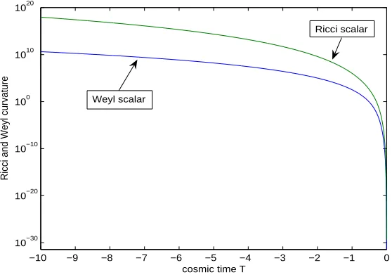
As has been pointed out by Penrose [46], the Weyl tensor does not directly affect the expansion of the universe, it, however, causes distortion which in turn leads to contraction. This implies a matter (i.e. Ricci) dominated initial Weyl curvature and a Weyl dominated Ricci curvature for the final stage of cosmic evolution [7]. The WCH, furthermore, indicates that any high-entropy singularity should lead to a very large Weyl curvature.

The WCH has influenced the definition of an IPS, given in the next section, and plays a significant role in shaping the definition for the cosmological futures, presented in chapter 8.

4.2 The definition

Scott [47] has removed some inherent redundancies of the original definition by Goode and Wainwright [8]. This amended definition provides a pattern in the quest for the definition of final states in this thesis and is given in Definition 4.1.

Definition 4.1 (Isotropic Past Singularity)

A space-time (_M,g) is said to admit an isotropic past singularity if there exists a space-time( ˜_M,g˜), a smooth cosmic time functionT defined on_M˜, and a conformal factor Ω (T) which satisfy

1. _M is the open submanifold T >0,

2. g = Ω2₍_T_{) ˜}_g _on _M_{, with} _g_˜ _{regular (at least} _C3 _{and non-degenerate) on an}

open neighbourhood of T = 0,

3. Ω (0) = 0 and ∃b >0 such that Ω∈C0_[0_{, b}_]_∩_C3₍₀_{, b}_] _and _{Ω (0}_{, b}_]_>₀_,

4. λ ≡ lim

T→0+L(T) exists, λ 6= 1, where L ≡ Ω00

Ω Ω Ω0

2

(34)

At this point it is necessary to better explain the definition of a cosmic time function [19, 47] used in the definition of the IPS as the literature tends to become rather inconsistent and sometimes mathematically unclean regarding the exact be-haviour of this function. Throughout this thesis the following definition will be used.

Definition 4.2 (Cosmic time function)

A cosmic time function is a function T on _M, which has a past directed timelike gradient ∇T with respect to g everywhere on M.

A theorem shall be given here which clarifies the characteristics of such a cosmic time function. The proof is based on [48].

Theorem 4.3

The cosmic time function T on _M increases along every future directed causal curve, the “slices” ST = {T = const} define a family of spacelike hypersurfaces

which foliate _M and to which _∇T is orthogonal. Every hypersurface _ST can only

be intersected once by a future directed causal curve.

Proof. Let γ : (a, b)_{→ M} be any future directed causal curve with tangent vector

γ0₍_t₎ ₆_{= 0. Then} _g₍_∇_T ₍_γ₍_t₎₎_{, γ}0₍_t_{)) =} _γ0₍_t_{) (}_T₎_> _{0 since} _∇_T _{is past directed and}

timelike. Thus, T must strictly increase alongγ. _∇T obviously must be orthogonal to the hypersurfaces ST and since ∇T is timelike the ST are spacelike. ∇T is

non-vanishing and dT is an exact 1-form. Therefore_Mcan be foliated by the_ST. AsT

strictly increases along any of these γ, it becomes clear that each of theses curves cannot intersect the ST more than once.

Hawking [19] has proven the important result that a space-time (_M,g) admits a cosmic time function if and only if it is stably causal (stable causality seems to be the appropriate condition for a space-time not to admit closed timelike curves, e.g. see Wald [21] and Ashley [49] for an interesting discussion).

Remark 4.4

Requiring the existence of a global time function T in the definition of an IPS is therefore equivalent to requiring stable causality on ( ˜M,g˜).

It is instructive, to interpret the definition of an IPS pictorially, as is done in Fig. (4.1). We will call the cosmological solution, (_M,g), of the EFE, the physical space-time, and, correspondingly, the conformally related space-time, ( ˜_M,g˜) - which does not necessarily describe a physically reasonable universe - will be referred to as the unphysical space-time. It is important to note that due to this shape of the definition one should think here of thephysical space-time to be produced from the

unphysical one, rather than vice-versa. In this sense the initial singularity in the

physical space-time is only due to the vanishing of Ω on the regular hypersurface

(35)

4.3. Isotropy and fluid flow 25

(M,g)

T = 0

Unphysical g = (T) g

( M, g)* *

space-time Physical

space-time

Ω Ω(0) = 0

[image:35.612.154.495.49.242.2]

2 _∗

Figure 4.1: Pictorial interpretation of the definition of an IPS (after Ericksson and Scott [9]). Note, that (∗_M_,∗_g_{) corresponds to our notation ( ˜}_M_,_˜_g_).

As will be seen in the next section, Definition 4.1 as it stands is not sufficient to guarantee an “isotropic” behaviour of the kinematics at the IPS. A further constraint on the fluid flow will solve the problem.

4.3 Isotropy and fluid flow

Now that the definition of an IPS stands, it is necessary to analyse how “isotropic” such a singularity is. To this end we first need to introduce the fluid flow.

4.3.1 The velocity vector field and the fluid flow

From observations of the almost isotropically distributed clusters of galaxies and their movement relative to us and to each other, it is well known that the general motion of matter around us is an overall expansion on large scales. Random velocities relative to the main movement are virtually negligible. This allows the definition of an average velocity vector ua_{, which represents the overall motion in}

our local vicinity [37]. Applying theCopernican Principle (see Introduction) to this vector implies its existence everywhere in the universe. Therefore we may assume the existence of a unique timelike vector field at every point in space-time which represents the average motion of matter. In order to admit comparisons of this vector field at different points of space-time we must normalise it, i.e.

uaua=−1. (4.5)

(36)

This velocity vector field ua _{defines a} _congruence _{in space-time.}

Definition 4.5 (Congruence)

Let O ⊂ M be open. A congruence in O is a family of curves such that through each p_{∈ O} there passes precisely one curve in this family.

Every continuous vector field - such as ua _{- generates a congruence of curves}

and, conversely, the tangents to a congruence define a vector field in _O [21]. The congruence generated by the velocity vector field ua _{is referred to as the fluid flow.}

4.3.2 Isotropy

In their seminal paper Goode and Wainwright [8] discuss three types of exact isotropy, all of which can be found in the FRW models†_{, in order to justify terming}

the singularities of Definition 4.1 “isotropic”.

(1) Weyl isotropy: Cabcd ≡0, i.e. there do not exist preferred directions due to the

principal null directions.

(2) Ricci isotropy relative tou(whereuis the timelike congruence defined in section 4.3.1): The anisotropic parts of the Ricci tensor relative to u vanish, Σa =

Σab ≡0 (see Appendix A.3 for a definition). The definition of Σa implies that

its vanishing makes u an eigenvector of Rab, while Σab = 0 guarantees that

the total projection ofRab orthogonal to u is isotropic.

(3) Kinematic isotropy relative to u: σ=ω = ˙ua_u_˙

a ≡0, i.e. the shear- and

vortic-ity eigenvectors, as well as the acceleration vector cannot define a preferred direction orthogonal tou.

One could require that the term “isotropic singularity” should only be given to singularities which satisfy the above types of isotropy. Restricting ourselves only to cosmologies as the FRW models, however, would not be helpful for studying the implications of quiescent cosmology and the WCH. Moreover, the universe is certainly not an exact FRW model‡_{and therefore we are interested in a more general}

class of models which do not exactly fulfil these types of isotropy.

The arguments in the introduction suggest models in which the shear, vorticity, acceleration and the anisotropic parts of the Ricci tensor are initially expansion-dominated. Unfortunately, Definition 4.1 as it stands, does not guarantee such a behaviour and thus allows singularities which are in no sense, isotropic, “quasi-isotropic” or “Friedmann-like”. The exact viscous fluid FRW cosmology by Coley and Tupper§_{[50] admits an IPS according to Definition 4.1, but does not satisfy the}

requirement of the expansion-dominated kinematics [8]. The fluid flow was shown

†_{see section 3.3.} ‡_{see section 3.4.}

§_{This solution of the EFE possesses an FRW metric but a different interpretation of the}

(37)

4.4. Gravitational entropy 27

not to be regular at the IPS in this model, which motivated Goode and Wainwright [8] to include the following definition.

Definition 4.6 (Fluid congruence)

With any timelike congruence u in _Mwe can associate a timelike congruence u˜ in

˜

M such that

˜

u= Ωu in M. (4.6)

(a) If we can choose u˜ to be regular (at least C3_{) on an open neighbourhood of}

T = 0 in _M˜, we say that u is regular at the isotropic past singularity. (b) If, in addition, u˜ is orthogonal to T = 0, we say that u is orthogonal to the

isotropic past singularity.

Note that the normal congruence to the slices always exists. Including this defi-nition turned out to be crucial for the framework of an IPS. Goode and Wainwright [8] proved that for a timelike congruence u which is orthogonal to the IPS, the following dimensionless scalars guarantee an asymptotic isotropy, in the sense that†

lim

T→0+

CabcdCabcd

RefRef

= 0, lim

T→0+ Σa_Σ

a

θ4 = 0, _Tlim_→₀+

ΣabΣba

θ4 = 0, (4.7) lim

T→0+

σ2

θ2 = 0, _Tlim_→₀+

ω2

θ2 = 0, _Tlim_→₀+ ˙

ua_u_˙ a

θ2 = 0. (4.8)

Quiescent cosmology only required that the initial state of the universe was similar to, but not exactly like an FRW model, in which these equations certainly hold. In this sense it is justified to term the more general singularities given by the con-junction of Definitions 4.1 and 4.6 “isotropic singularities” to distinguish them from singularities in models which are useless for this scenario. Henceforth it is this con-junction which is meant when we refer to the definition of an IPS. This definition implies a number of physically significant results which will be discussed in the next section and in chapter 5. The slight anisotropy allowed on the sliceT = 0 turns out to be crucial for the explanation of galaxy formation (see section 5.1). As will be seen in chapter 8, Definition 4.6 will moreover become essential in the treatment of future singularities.

4.4 Gravitational entropy

The strongest version of the Weyl Curvature Hypothesis (WCH) suggests that the Weyl tensor must have been identical to zero at the beginning of the universe, to guarantee a complete absence of clumping. This is, however, a too stringent constraint on the initial state of the universe; Tod [51] has conjectured that there are no non-FRW models that admit an IPS and also satisfy the strongest version

(38)

of the WCH. This view has been supported in an analysis by Goode [52], who showed that in the case of a geodesic fluid the initial condition of a vanishing Weyl tensor in the physical space-time admits the solution of a vanishing Weyl tensor throughout the cosmology - which corresponds to an FRW model - the uniqueness of this solution, however, has not yet been confirmed.

Nevertheless, in this light the strongest version of the WHC does not seem physically plausible, since more general cosmologies than exact FRW models will be necessary for describing the overall evolution of our universe†_{. As briefly discussed in}

section 4.1 Penrose [7] suggested that the Weyl curvature should be Ricci dominated at an initial singularity and that the converse should be true for higher entropy states at later stages of cosmic evolution. The easiest way to encode this into formulae is via the following dimensionless scalar

K = CabcdC

abcd

RefRef

, (4.9)

which is the simplest possible measure of the relative significance of the Weyl and Ricci curvatures. In section 4.3.2 it was already seen that in general at an IPS

lim

T→0+K = 0. (4.10)

An instructive proof of this behaviour will be given in section 10.1, as a by-product of a more general theorem also concerning this ratio for possible future singularities. In the light of Penrose’s suggestion, equation (4.10) seems to be an appropriate initial boundary condition for the universe - i.e. an appropriate version of the WCH - which will not only be satisfied by the FRW models, but by a much wider class of physically more reasonable cosmologies.

Goode, Coley and Wainwright [12] have started to investigate whether the scalar

K could be an appropriate measure of gravitational entropy, i.e. whether

∂uK >0 (4.11)

where∂u means differentiation along the fluid congruence. The direction of

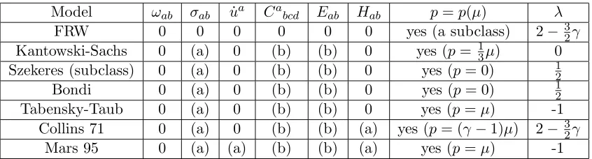
increas-ing K would then determine a gravitational arrow of time. In [12] it is suggested to investigate the validity of equation (4.11) in the full class of cosmologies which admit an IPS. At this point we can already state that equation (4.11) does not hold in FRW universes in whichK ≡0. Nevertheless, equation (4.11) could be confirmed for all of cosmic time in several non-FRW models, e.g. the Szekeres dust solutions and the Kantowski-Sachs models which admit an IPS (see chapter 7) among others [12]. In some classes of the Bianchi models which admit an IPS, however, it depends on the exact shape of the γ-law equation of state as to whether K monotonically increases along the fluid flow for all times [12]. It remains an open task to give a general answer to this behaviour. Moreover, no other clear-cut formula has been found so far which gives a measure of gravitational entropy.

Encoding Possible Final States of the Universe with Conformal Structures