The atomic waveplate

(1)

The Atomic Waveplate

A thesis submitted as partial fulfillment of the requirements for the degree of Bachelor of Science with Honours in Theoretical Physics at

the Australian National University

Peter Kuffner

(2)

(3)

Declaration

This thesis is an account of research undertaken under the supervision of Dr John Close and Dr Joseph Hope, between January and November 2003 in the Atom Optics group at the Department of Physics and Theoretical Physics, in the Faculty of Science of the Australian National University. Except where acknowledged in the customary manner, the material presented in this thesis is my own work.

Peter Kuffner November, 2003

(4)

(5)

Acknowledgements

A number of people deserve my thanks for their help, friendship and tolerance during the course of my honours year.

I would like to thank my supervisor, Dr John Close, for his helpful (and occasionally not so helpful) guidance in the course of my project. Never too shy to jump into the office and, looking deviously, ask the question ‘So Peter, what have you accomplished today?’, Crazy John has been a real motivator in my work. At the same time I am grateful for Johns patience with me, every time I wandered into his office and announced that it was ‘Stupid Question Time!’.

Many thanks go to Simon Haine, without whose help I would have taken a long time to learn some of the intricacies of numerical modelling. Simon was great not only for his help, but also for his many renditions of the ‘Rain Song’, a tune that I’m going to need a lobotomy to remove from my brain.

I would like to thank Dr Joe Hope, the Giver Of CPU Time, and official Mathematica Guru, for his help with many computer issues (and help with physics occasionally! hehe!). While his patience with Stupid Question Time! was great, ‘There are no stupid questions, just stupid people’, just doesn’t cut it in my opinion. Joe’s crazy humour and steady discouragement helped calm my nerves before my honours talks, for which I am grateful.

Throughout my honours year, and especially during lunch time, Craig Savage has been an inspiration. His (slightly unhinged) passion for physics and anything in general was great to behold, especially during the quantum mechanics course. Mentioning courses, Aiden Byrne, the Master of Three Angular Momenta, has my thanks for making what appears to be a dry subject quite interesting.

I need to thank the whole atom optics group for their friendship and musical randomness. Thanks to John, Joe, Simon, Adele, Dr Nick, Cameron, Michael, Craig, StealthPearl, and Panda. I look forward to seeing Simon and Johnfunkel playing live to a crowd of tens one day.

I probably shouldn’t thank Annoying Kurt, but this is an acknowledgments section and I should acknowledge his periodic but immense (and occasionally humorous) annoyance. Thanks for putting your toesocked foot down, Adele.

Thanks to dodgy Stu and Magnus, for your...well...randomness I guess.

Thanks to Lunchtime for keeping me amused (and fed), but it wouldn’t have been the same without all the physicists present. Thanks to Susan, Craig, Joe, John, Ping Koy and anyone else who had something opinionated and interesting to say while we all ate.

My family has been immensely supportive during the year and I would like to thank them for feeding and tolerating me in times of stress when I was preparing talks and writing this thesis. I guess I have to thank my brother at some point...might as well be here. His incessant bad jokes and good humour kept me sane at times when I could have gone mad checking for errant (and sometimes mythical) factors of a 1₂ in my work.

(6)

(7)

Abstract

In this thesis, we theoretically model the behaviour of atoms outcoupled from an atom laser passing through an RF resonance. Within the Landau-Zener formalism, we find a range for the Rabi frequency of the RF field, inside of which dynamical spin transitions occur. We find that atoms exiting the resonance region exhibit symmetric transition into trapped and untrapped spin states. A further numerical model, within the mean field approximation, is performed for an atomic pulse from an atom laser passing through the resonance. The extra coupling between states introduced by the spatial extent of the pulse causes a spread in the momentum of trapped and anti-trapped states that atoms are coupled into within the resonance. An experimental setup for the manipulation of the atomic spin states with an RF field is investigated and designed. The implications of these results is discussed regarding the design of a pumped atom laser using continuous RF evaporation.

(8)

(9)

Introduction

1.1 Overview of this chapter

In this introductory chapter, we briefly discuss the field of atom optics and the nature of atom lasers. We follow this with a discussion of radio frequency field techniques in atom optics and the concept of the atomic waveplate. The goals of this thesis are explained, with an eye to answering an additional question about a possible continuous atom laser design. An outline of the rest of this thesis follows this.

1.2 The Field of Atom Optics

Inspired by the wave-particle duality for light, the wavelike nature of atoms was first postulated by de Broglie [1], and subsequently demonstrated by Stern [2]. This lead to a major change in the thought about how matter behaved, with atoms now being described as matter-waves characterised by their wavelength, λ = h_p, where h is Planck’s constant and p is the particle’s momentum. Combined with Heisenberg’s uncertainty principle, this meant that as momentum uncertainty is reduced, a particles uncertainty in position increases. A particle that might have a definite position in space loses this as its momentum uncertainty is reduced, instead having a spatial extent given by the de Broglie wavelength.

For a long time the scale of this wavelength was too small to be of much use, due to the large momentum of the particles involved. Observation of atomic waves was restricted to the realm of electron interferometry and related experiments. Since the laser cooling of atoms below the photon recoil limit [3], however, this wavelike nature has been large enough to become of practical interest. As atomic cooling techniques have improved, the Bose condensed gas has been achieved, creating a ready source of matter-waves, With this, the field of atom optics was recognised. This is a growing field of physics involving the investigation and manipulation of these matter-waves, in an analogous manner to the manipulation of light.

Many things have been achieved in this field recently, with several experimental demonstra-tions of the appropriately named atom laser [4, 5]. This has given physicists a coherent beam of bose condensed atoms, a short-lived standing or pulsed matter-wave, with which experiments can be performed. While one of the key research goals in atom optics is developing the continuously pumped atom laser, investigation into the manipulation of atom laser beams proceeds apace. We have seen reflection, focusing, beamsplitting and polarisation of these coherent atomic waves [6]. These are only basic atom optics experiments, however, and more research in this field is needed before atom lasers become useful tools.

(12)

2 Introduction

1.3 BEC - The Bose Gas

A significant source of matter-waves for atom optics experiments is the Bose-Einstein Condensate (BEC). This is essentially a cooled gas of atoms that has undergone a quantum phase transition, coalescing into a quantum matter-wave. This phenomenon was first proposed by Einstein [7], building on the work done by Bose on the statistics of identical particles. This theory produced the non-classical Bose-Einstein distribution function for a system of N non-interacting bosons. These are particles with integer spin, whose wavefunctions are symmetric under interchange. For the Bose-Einstein distribution, the following critical temperature was shown to exist

Tc ≈3.3 ¯

h2 kBM

n2/3 (1.1)

where M is the mass of each particle, and n is the number density. Below this critical temperature,

N0particles in the system are statistically driven into the lowest energy state for a single particle, without an attractive force. This fraction of the total particles reaching their ground state is given by

N0 =N 1−

_T

Tc

3/2!

(1.2)

where the temperature dependence shows this condensed fraction increasing in number with further cooling. The critical temperature for condensation coincides with the temperature range where the de Broglie wavelength of atoms is of the order of the interatomic separation. Bosonic atoms in the condensate act as atomic wave packets, each in their ground state and overlapping with their neighbour, resulting in a quantum fluid of particles.

The first experimental evidence for BEC appeared in superfluid helium, and this seemed to be the only exception to the rule that matter would freeze before it could be cooled to the critical temperature for condensation. With laser and evaporative cooling of alkali atoms in their gaseous state, this all changed, and the condensate was realised for atoms confined inside magneto optic traps [8]. This has given physicists a most interesting system to study; a macroscopic quantum system composed of matter waves.

1.4 Atom Lasers

One of the recent developments in atom optics is that of the atom laser, a device created from the manipulation of BEC that is the atomic analogue of the optical laser. When one neglects the gain, loss and pumping mechanisms, the simplest picture of an optical laser becomes that shown in figure 1.1. This is simply a resonant cavity created by two mirrors, in which photons (bosons) oscillate back and forth, with a certain probability of exiting through a partially silvered mirror. The photons in the cavity interfere with one another, ensuring that one of the excited state cavity modes is macroscopically occupied. We call this the lasing mode, and a coherent beam of photons is emitted from this cavity in the lasing mode.

(13)

[image:13.595.192.442.121.190.2]

§1.4 Atom Lasers 3

Figure 1.1: An optical laser. This picture just shows the resonant cavity and the excited lasing mode, ignoring the pumping and amplification mechanisms. Photons are outcoupled via the partially silvered mirror, creating a coherent beam

changing the atoms magnetic spin states, keeping the atoms in the energetic ground state, but changing their dipole interaction with the magnetic trapping potential. This has been done with radio frequency fields [9], and Raman transitions [10]. Once this is done, a coherent atomic wave is created, which is generally left to fall under gravity.

Figure 1.2: An atom laser alongside an atom laser cavity. Atoms from a BEC occupy the lowest energy state of the cavity defined by the magnetic trap. An atomic beam is created by active transition of atoms from a trapped state,|Ti, to an un-trapped state,|Ui, within the system by manipulation of atoms magnetic spin states. This creates a temporally and spatially coherent matter wave as the atoms fall under gravity.

Matter wave beams from an atom laser show spatial coherence just as optical beams do. The polarisation of an optical beam is a vector quantity carried by the field, and so atomic beams contain polarisation in an analogous fashion. In this case, the polarisation is given by the spin states of the atoms within the beam.

It is the differences between an atom laser and an optical laser that make it most interesting, however. Matter-wave beams show non-linear effects even in vacuum, due to the inter-atomic interactions that are still present. While the wavelength of an atom laser is large enough to be useful, atom laser beams are produced with much shorter wavelengths than optical beams. These beams possess more varied polarisation states than the two orthogonal ones possessed by their optical counterpart, making for a more complex polarisation behaviour.

[image:13.595.122.500.368.517.2]

(14)

4 Introduction

continuous pumping mechanisms possessed by optical lasers. This is where the analogy breaks down, as many consider a real model of an optical laser to fundamentally include pumping, gain and loss mechanisms. This will hopefully be rectified by physicists in the near future.

1.5 The Atomic Waveplate

In optics, one of the most fundamental devices is the waveplate, a device that changes the polar-isation of an incident beam. When one adds a beamsplitter into the system after the waveplate, one can control the intensities of the two output beams. This polarising beamsplitter forms a fundamental component in many interferometers, including the new gravitational wave detectors under construction. Such devices are missing in atom optics, needing to be designed from scratch. If we wish to make an analogous device for atom optics, we are envisioning something that can control the intensities of the atomic polarisations; the spin states. Control of these spin states is already fundamental to atom optics, through the use of radio frequency fields in the operation of atom lasers.

These RF fields are used to manipulate the spin states of atoms, transferring trapped atoms to un-trapped states within magnetic traps, and are popular due to their simplicity over other schemes. RF evaporation has so far been the best way of cooling an atomic cloud the final amount needed to obtain BEC [11]. Similarly, the RF outcoupler created by Meweset al [12] is currently the easiest way of obtaining an atom laser beam.

[image:14.595.187.394.485.679.2]

The focus of this thesis is an investigation of the behaviour of atoms in RF fields with an eye to creating an atomic analogue to the waveplate. This atomic waveplate is shown in figure 1.3 where we are applying an RF field across the path of an atomic beam, creating a resonance region. Atoms enter the resonance in their untrapped polarisation state, and may exit the region

Figure 1.3: The atomic waveplate. A radio frequency field is applied across the path of a falling atom laser beam. Atoms entering the resonance in a particular spin state can be transferred to another possible spin state upon exiting the region. Control of the way atoms are spin flipped would produce a device for use in the atom optics field.

(15)

§1.6 The Continuous Atom Laser 5

The application of this RF field must be done with care, since any component of this field that happens to lie in the same direction as that of the magnetic trap field will simply add with the trap field, either strengthening or weakening the trap (depending on whether it is in the +ve or -ve direction. This means that the applied RF field must be perpendicular to the magnetic trap field in order to create the effect we desire.

We wish to understand the dynamics of atoms within the resonance region, in order to see if we can control the probability of atoms exiting the resonance in different spin states. This would provide an atom optics device analogous to the optical waveplate.

1.6 The Continuous Atom Laser

This thesis also aims to answer another question. As mentioned in the earlier, one of the major goals in atom optics is the construction of a continuously pumped atom laser.

[image:15.595.182.448.374.555.2]

In a continuously pumped atom laser, atoms must be cooled down and pumped into the BEC from a reservoir, at the same time as atoms are outcoupled from the magnetic trap. One scheme one considered by the ANU atom optics group for accomplishing this, is to combine the RF fields for outcoupling and evaporation. A simple picture of this is shown in figure 1.4. Atoms are

Figure 1.4: Simple scheme for a continuous atom laser. Atoms are continuously RF evaporation cooled down to BEC temperature from a surrounding cloud of thermal atoms. Atoms are also RF outcoupled from the condensate at the same time. We also include the RF resonance from the waveplate in the picture.

(16)

6 Introduction

This thesis aims to investigate the behaviour of atoms within these RF fields, answering the possibility of creating an atomic waveplate as well as seeing if the continuous atom laser presented here is viable.

1.7 Overview of this thesis

In chapter 2, we complete a full analytic investigation of simple 2 level atoms passing through an RF resonance. We use the dressed state formalism to introduce the Landau-Zener avoided crossing picture of the dynamics.

After this, chapter 3 investigates the atomic waveplate for the more complex atom of rubidium, with the difficulty in solving the problem leading to numeric modelling of the atoms behaviour. We show the effect on the atoms of varying the strength of the applied field, finding a symmetric transfer of atoms into different states and a maximum field strength that produces the same effect as for no applied field.

Chapter 4 is a numerical investigation into the behaviour of a full atomic wavepacket passing through the RF resonance region, showing the atomic beamsplitting within a GP formalism for the dynamics.

The experimental design for the atomic waveplate is covered in chapter 5. We classify the experimental requirements, where the low B field and high current strengths needed lead to the design of an efficient resonant circuit to power the RF coil.

(17)

Chapter 2

Atoms in RF fields

2.1 Overview of this chapter

In this chapter, we consider a first investigation of the behaviour of atoms in RF fields, using a simple two level atomic system. The system’s behaviour in the vicinity of an avoided energy level crossing is studied in detail, through the semi-classical dressed state formalism, before being compared to a simple scaling model.

2.2 Understanding Atoms in RF fields

In order to create a useful device through the application of an RF field to an atomic beam, we must first understand the behaviour of atoms within the field. Atoms outcoupled from the magnetic trap will fall under gravity, passing into resonance with the RF field, whilst still within the field created by the magnetic trap. This means that the atoms feel both of the magnetic fields in the resonance, and so we must understand the dynamics of atoms within the combined magnetic fields.

We wish to gain a basic understanding of atoms in RF fields, and so we start with a theoretical investigation into the behaviour of 2 level atoms in the fields necessary for the waveplate. This system has the advantage of being analytically solvable and is an easy way of introducing the concepts required for a dynamical understanding of the RF interaction. BEC is the quantum degeneracy of bosonic particles, however, and this analysis will not give us a full understanding of our atomic waveplate, as two level systems are fermionic. What the analysis does give us, is an understanding of the physics involved, since as we will see in the next chapter, the real bosonic system is too complex to obtain an analytic solution of the behaviour.

2.3 Two Level Investigation of a Landau-Zener Avoided Crossing

In this theoretical investigation, a first approximation of the atomic system is to that of the energetically degenerate two level atom, a classic example of which is the spin 1/2 electron. In this case, we consider the light field classically, so that the interaction between the atom and the field is simply given by a semi-classical dipole interaction.

Because of both the strength of the magnetic field from the trap, and the close positioning of the RF resonance, the atom interacts with the fields of both the magnetic trap and the incoming radio-frequency photon, and so the Hamiltonian is given by

ˆ

H =₋~µ_·B~0(ˆz)ˆz−~µ·B~1cos(ωt)ˆx= −

egs

2m B0(ˆz) ˆSz+

−egs

2m B1cos(ωt) ˆSx (2.1)

(18)

8 Atoms in RF fields

where ˆSz and ˆSx = 1₂( ˆS+ + ˆS−) are the spin projection operators in the z and x directions respectively.

h

ωrf

h

∆

(z)

h

ω0

(z) |2>

|1>

E

[image:18.595.191.379.164.279.2]

0

Figure 2.1: The Zeeman split energy states of the 2 level system, around z = 0. We introduce the detuning, ∆(z), as the frequency difference between the Zeeman shift,ω0(z), and the incoming photon,ω

The first term is the interaction with the spatially varying trap field, and the second is the time varying photon interaction. Note that the applied field, B1, is polarised in the x direction, orthogonal to the magnetic trap field, B0, as mentioned in the introduction. The trap field results in a Zeeman splitting of the atomic energy levels, lifting their degeneracy. A picture of this interaction is shown in figure 2.1 with the two orthogonal energy states _|2_i = _|1₂,1₂_i and |1_i=_|1₂,₋1₂_i. In this semi-classical description, we use the completeness requirement

n

X

i=1

|φiihφi|= 1 (2.2)

to express this Hamiltonian in the projection operator formalism as

ˆ

H = ¯h

2ω0(z)(|2ih2| − |1ih1|) + ¯

h

2ω1cos(ωt)(|2ih1|+|1ih2|) (2.3)

with ω0(z) = ∆(z) +ω. where the spin raising and lowering operators,

S_±|s, msi= ¯h

q

s(s+ 1)₋ms(ms+ 1)|s,(ms±1)i (2.4)

have introduced a factor of√2 in the cosine term when operating on our states. This factor has been subsumed into the equations, along with a factor of 1₂ generated from the Fx operator.

The frequency ω0(z) is related to the magnetic trap field by ω0(z) = _¯_h1µbgsB0. Similarly,

ω1= _¯_h1µbgsB1, and is known as the Rabi frequency, the frequency at which an atom’s spin state changes in the presence of an applied RF field.

Before we solve for the dynamics of this system, we transform to an interaction picture, first splitting our Hamiltonian into two terms,

ˆ

H0= ¯

h

2ω(|2ih2| − |1ih1|) (2.5)

and

ˆ

V = ¯h

2∆(z)(|2ih2| − |1ih1|) + ¯

h

(19)

§2.3 Two Level Investigation of a Landau-Zener Avoided Crossing 9

and then using the unitary transformation

ˆ

HI=eiHˆ0t/¯hV eˆ −iHˆ0t/¯h (2.7) The interaction Hamiltonian is then

ˆ

HI = ¯

h

2∆(z)

eiωt/2_|2_ih2_|e−iωt/2₋e−iωt/2_|1_ih1_|eiωt/2 (2.8) +¯h

2ω1cos(ωt)

eiωt/2_|2_ih1_|eiωt/2 +e−iωt/2_|1_ih2_|e−iωt/2 (2.9) = ¯h

2∆(z) (|2ih2| − |1ih1|) + ¯

h

4ω1

(e2iωt+ 1)_|2_ih1_|+ (e−2iωt+ 1)_|1_ih2_| (2.10)

= ¯h

2∆(z) (|2ih2| − |1ih1|) + ¯

h

4ω1(|2ih1|+|1ih2|) (2.11)

where we have made the rotating wave approximation by neglecting the fast time dependence terms ofe2iωt _and_e−2iωt_{. After this, the interaction Hamiltonian in matrix form is}

ˆ

HI= ¯

h

2

∆(z) ω1 2 ω1

2 −∆(z)

!

(2.12)

Eigenvalues of this Hamiltonian are q∆(z)2_{+ (}ω1

2 )2 and −

q

∆(z)2_{+ (}ω1

2 )2. Figure 2.2 shows

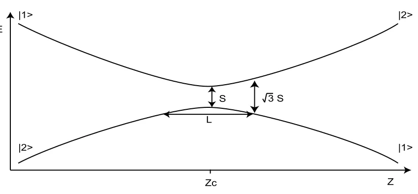
|1> |2> |2> S L |1> 3 S

Zc Z

[image:19.595.88.512.406.603.2]

E

Figure 2.2: Simplified plot of a Landau-Zener avoided crossing. An atom initially in one of the spin states, eg state |2i, falls under gravity until entering the avoided crossing region, characterised by its length, L, and separation, S. Exiting the region, an atom may either adiabatically follow the energy eigenstate, finishing in state|1i, or it may make a non-adiabatic energy transition, finishing in state|2i.

(20)

transition to the _|2_i state. However, in order for the atom to make such a spin flip, it must adiabatically follow the dressed energy state through the interaction. Similarly, for the atom to remain in the same spin state it must make a non-adiabatic transition to the other dressed state, after passing through the resonance.

2.4 Interaction Picture Dynamics

Now we examine the time evolution of the system, given by the equation

ˆ

HI|Ψ(t)i=i¯h∂|Ψ(t)i

∂t (2.13)

In solving the time evolution we consider a single atom falling under gravity, following a classical trajectory. In this case, our detuning function ∆(z), may be expressed as a function of time, ∆(t), as z = 1₂gt2_{. Our schr¨odinger equation may now be solved by taking our general state} |Ψ(t)_i, as

|Ψ(t)_i=C1(t)e−i

Rt

0∆(t)/2 dt 0

|1_i+C2(t)ei

Rt

0∆(t)/2 dt 0

|2_i (2.14)

following the method used by Rubbmark [13]. Substituting this state into our evolution equation yields the following coupled differential equations

iC˙1 =

ω1 4 e

iR₀t∆(t)/2 dt0

C2 (2.15)

iC˙2 =

ω1 4 e

−iR₀t∆(t)/2 dt0

C1 (2.16)

Decoupling these gives a pair of second order differential equations

¨

C1−i ∆(t)

2 C˙1+

ω2 1

16C1= 0 (2.17)

¨

C2+i ∆(t)

2 C˙2+

ω2 1

16C2= 0 (2.18)

Now, making the approximation that ∆(t) varies linearly in time in through the avoided crossing, this system can be solved using the method by Zener [14]. This last approximation is reasonable for the case of an atom falling under gravity. Its implication is that an atom will traverse the crossing in a very small space of time, and later we will see that this is quite true. The result is the following function, giving the probability of a non-adiabatic transition between dressed energy states.

P =e−2πΓ (2.19)

Where Γ is given by the ratio of the avoided crossing’s height to it’s length parameter,

Γ = |h1|Vˆ|2i| 2

¯

h2∂∆(t)_∂t

tc

(2.20)

2.5 Parameterising The Solution

(21)

§2.5 Parameterising The Solution 11

the system simply by setting our magnetic field parameters.

The first thing to do is to define the detuning. Remembering that ∆(z) = ω0(z)−ω and seeing that the magnetic trap is an Ioffe-Pritchard type of trap (specifically a QUIC trap [15]). The total magnetic field in the z direction from the I-P trap is harmonic, however, we consider the position of the avoided crossing as far from the centre of the trap. In this case, the field may be approximated as varying linearly in space in the region of the avoided crossing. Our ω0(z), and hence detuning, can now be redefined.

ω0(z) =α(z−zc) +ω (2.21)

∆(z) =α(z₋zc) (2.22)

where the introduction ofzc defines the position of the RF field resonance, and thus the position of the avoided crossing, in space.

This enables us to parameterise the probability function obtained in the previous section, and the avoided crossings’ length and separation. Firstly, we can see that ∂∆(t)_∂t = ∂∆(z)_∂z ∂z_∂t, where

α = _¯_h1µbgs∂B_∂z0 is the magnetic field frequency gradient and ∂z_∂t =v is the atom’s velocity. And we can now re-express Γ,

Γ = ω 2 1

16αv (2.23)

and the corresponding probability function

P =e−π ω2

1

8αv (2.24)

Looking at the detuning function, ∆(z) =ω0(z)₋ω=α(z₋zc), we can solve for the position of the avoided crossing. It is given by

zc =

ω₋ω0(z= 0)

α (2.25)

meaning that the crossing position is determined simply by the RF fields’ frequency, once the magnetic trap field is fixed. Increasing this frequency lowers the position in space, moving it further from the trap centre.

The avoided crossing level separation, S, that we defined in figure 2.2 can be found by looking at the the energy eigenvalues of ˆHI. These are±

q

∆(z)2_{+ (}ω1

2 )2, and at the resonance, detuning is zero. So the separation is

S= 2_|h1_|Vˆ_|2_i|= ¯hω1

2 (2.26)

and is simply the strength of the RF field interaction.

Lastly, we find L, the parameter that characterises the width of the avoided crossing. This was defined as the ratio of the crossing height (or level separation) to the gradient of the crossing around the critical point

L= 2|h1|Vˆ|2i| ¯

h∂∆(z)_∂z

zc

= ω1

2α (2.27)

And appears in figure 2.2, as twice the distance over which the energy eigenvalue separation changes from S to √3S.

(22)

a greater probability of adiabatically following its dressed state, and so a greater probability of making a spin flip as it passes through the crossing. The other parameters that affect the probability are the atomic velocity and α. These parameters will be fixed when we make the atomic waveplate, by simply fixing both the position of the avoided crossing in space, and the magnetic trap gradient. This will simplify repeated experiments since the dynamics will always occur in the same place and detection apparatus need not be adjusted.

2.6 Simple Scaling Model

Here we explain the dynamics with a simple scaling model. We have obtained a probability function

P =e−π ω2

1

8αv (2.28)

that gives us the probability of an atom making a non-adiabatic transition to another dressed state. In this system the Rabi frequency is the key to the dynamics.

But what does it mean for an atom to make a transition from one dressed state to another? Consider the following argument. When an atom traverses the avoided crossing there will be, at best, a time energy uncertainty of ∆E∆t= ¯h₂. Now ∆t= L_v, simply the time it takes to traverse a crossing of width L, at velocity v. This gives an energy level difference of ∆E= v

2L, and given that L= ω1

2α, we now have

∆E = ¯hαv

ω1

(2.29)

Now we can express the atomic energy uncertainty as a number of crossing separations, ∆E =

k¯hω1

2 , were k is a constant. Solving the resulting equation forω1, yields

ω1=

r

2αv

k (2.30)

If we substitute this ω1 into the probability function from the analytic solution, we get

P =e−π4k (2.31)

Looking at this function, as k _{→ ∞}, P _→ 1, and as k_→ 0, P _→ 0. This really means that if ∆E ¯hω1

2 thenP ≈1, and if ∆E¯hω 1

2 thenP ≈0.

We now have a simple scaling model: If the uncertainty in the atoms energy is greater than the avoided crossing energy separation, then the atom will make a non-adiabatic dressed state transition. This corresponds to no spin flip in the atomic state as explained earlier. This means that the atomic energy uncertainty must be less than the crossing energy separation if we want the atom to undergo a spin flip as it passes through the resonance.

2.7 Conclusion

(23)

Chapter 3

Rubidium in RF Fields - The 3 & 5

Level Atoms

3.1 Overview of this chapter

in this chapter we apply the analytic method used in the previous chapter to the actual atomic species to be used in an atomic waveplate experiment. Finding the subsequent systems fundamen-tally too difficult to solve analytically, we then numerically integrate them, obtaining solutions for their behaviour, after testing the algorithm against the analytic solution for the 2 level atom.

3.2 Rubidium 87 Structure in the Presence of RF Fields

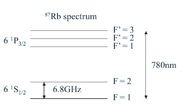
The atomic species used here at the ANU is rubidium 87, part of the spectrum of which is shown in figure 3.1. The ground state of rubidium is hyperfine split into two levels separated by 6.8GHz. This creates two possible states for creating BEC in, the F = 1 or the F = 2 states. In the presence of the magnetic trapping field, however, these states are further Zeeman split into their magnetic sublevels, the_|F, Mfi states. The F = 1 state becomes the set of states|1,(±1,0)i, while the F = 2 state splits into_|1,(_±2,_±1,0)_i. This means our experiment can be effectively be carried out with two types of atoms, the F = 1 three level atom, and the F = 2 five level atom.

This gives us a real picture of the atomic waveplate. Atomic pulses are outcoupled from the magnetic trap in the_|0_istate of whichever F state is chosen to do the experiment in. These atoms then fall under gravity passing through the resonance region, where they may be spin flipped into other magnetic sublevels. What is important, is that each of the magnetic sublevels interacts with the magnetic trap potential in different ways. Since the_|0_i state simply falls under gravity, this is the reason we choose to outcouple into this state. The other states interact differently.

For the 3 level atom, the _|+Mfi states are anti-trapped by the potential, and will be accelerated along the magnetic trap’s field lines. In the case of an atom laser at the ANU, this is just along the atoms initial trajectory, falling downwards. The_{| −}Mfi states are trapped by the potential, meaning that any atoms flipped into these states will reverse their trajectory, being pulled back towards he centre of the trap. This is reversed for the 5 level atom, though, with the |+Mfistates trapped by the potential, and the | −Mfianti-trapped.

3.3 3 & 5 level atom dynamics in the Landau-Zener avoided

crossing

Now we investigate the dynamics for our rubidium atoms, using the method that proved successful for the 2 level atomic analysis.

(24)

[image:24.595.135.437.111.290.2]

14 Rubidium in RF Fields - The 3 & 5 Level Atoms

Figure 3.1: Picture of the ground and first excited states of rubidium. The ground and first excited state have been split by the hyperfine interaction between the nucleus’ and the valence electron’s magnetic dipole moments.

Atoms in the F = 1 hyperfine state have their states expressed as: _|1_i = _|1,1_i, _|0_i =_|1,0_i, | −1_i=_|1,₋1_i. We perform the same analysis for this system as was done for the 2 level atom, so our Hamiltonian starts as a dipole interaction,

ˆ

H=₋~µ_·B~0(ˆz)ˆz₋~µ_·B~1cos(ωt)ˆx= −

egf

2m B0(ˆz) ˆFz+

−egf

2m B1cos(ωt) ˆFx (3.1)

where ˆFz and ˆFx = 1₂(F+ +F−) are the total angular momentum operators in the z and x directions respectively. We make the same linearity approximation for ω0(z), as well as the classical trajectory approach for the atoms as we did for the 2 level atom. Using the completeness requirement,Pn

i=1|φiihφi|= 1, we express this hamiltonian in the projection operator formalism as,

ˆ

H= ¯hω0(t)(|1ih1| − | −1ih−1|) + ¯

h

√

2ω1cos(ωt)(|0ih−1|+| −1ih0|+|0ih1|+|1ih0|) (3.2)

where the raising and lowering operators,

F_±|F, Mfi= ¯h

q

F(F + 1)₋Mf(Mf + 1)|F,(Mf ±1)i (3.3)

have introduced the factor of √2 in the cosine term when operating on our states. This factor has been subsumed into the equation, along with a factor of 1₂ generated from the Fx operator.

Note that ω0(z) = ∆(z) +ω, ω0(z) = 1_¯_hµbgsB0 and ω1 = _h_¯1µbgsB1, as before. Here we note that only the nearest states are coupled, so the _|0_i state couples to both the_|1_iand _{| −}1_i states, while the_|1_i state does not directly couple to the _{| −}1_i state.

We now transform to the same interaction picture as previously by splitting our hamiltonian into two parts

ˆ

(25)

§3.3 3 & 5 level atom dynamics in the Landau-Zener avoided crossing 15

and

ˆ

V = ¯h∆(z)(_|1_ih1_{| − | −}1_ih−1_|) +_√¯h

2ω1cos(|0ih−1|+| −1ih0|+|0ih1|+|1ih0|) (3.5)

Where the interaction picture hamiltonian is defined by the unitary transformation

ˆ

HI=eiHˆ0t/¯hV eˆ −iHˆ0t/¯h (3.6) We also make the rotating wave approximation. The final interaction hamiltonian is

ˆ

HI = ¯h



  

∆(z) ω1 √ 8 0 ω1 √ 8 0 ω1 √ 8 0 ω1

√

8 −∆(z)



  

(3.7)

where we have included the extra factors of 1₂ resulting from this transformation.

Now, once again, we consider our atoms falling under gravity, following a classical trajectory. The detuning function ∆(z), is then expressed as a function of time, ∆(t), asz= 1₂gt2.

We now perform the time evolution through the following equation,

ˆ

HI|Ψ(t)i=i¯h

∂_|Ψ(t)_i

∂t (3.8)

choosing our general state to be the same as previously

|Ψ(t)_i=X m

Cm(t)e−im

Rt 0∆(t) dt

0

|m_i (3.9)

wherem signifies theMf number for each of the three states.

This results in the following set of coupled differential equations

iC˙1=

ω1 √

8e

iR₀t∆(t)dt0

C0 (3.10)

iC˙0 =

ω1 √

8

e−iR

t 0∆(t) dt

0

C1+ei

Rt 0∆(t) dt

0

C₋1

(3.11)

iC˙₋1=

ω1 √

8e

−iR₀t∆(t)dt0

C0 (3.12)

At this point the problem ceases to be solvable analytically, since it is too difficult for the differential equations to be decoupled and solved. This is despite the possibility of choosing another generalised state, or even another interaction picture, since the detuning carries some of the time dependence for which we wish to solve. The detuning always remains, in some form, along the main diagonal of the hamiltonian matrix.

(26)

The five level atom interaction hamiltonian is given by

ˆ

HI = ¯h

         

2∆(z) ω1

2 0 0 0

ω1

2 ∆(z)

q

3

8ω1 0 0

0 q3₈ω1 0

q

3

8ω1 0 0 0 q3₈ω1 −∆(z) ω₂1

0 0 0 ω1

2 −2∆(z)

          (3.13)

Where the spin raising and lowering operators have introduced factors of 2 and√6 when operating on our states. These factors have been subsumed into the hamiltonian, along with two factors of

1

2 generated from the interaction transformation and theFx operator.

Making the same approximations, and carrying out time evolution on our generalised state, results in the following differential system

iC˙2=

ω1 2 e

iR₀t∆(t)dt0

C1 (3.14)

iC˙1 =

ω1 2 e

−iR₀t∆(t) dt0

C2+

r

3 8ω1e

iR₀t∆(t)dt0

C0 (3.15)

iC˙0 =

r

3 8ω1

e−iR

t 0∆(t)dt

0

C1+ei

Rt 0∆(t) dt

0

C₋1

(3.16)

iC˙1=

ω1 2 e

iR₀t∆(t)dt0

C₋2+

r

3 8ω1e

−iR₀t∆(t)dt0

C0 (3.17)

iC˙₋2 =

ω1 2 e

−iR₀t∆(t)dt0

C₋1 (3.18)

This system is not solvable for the same reasons as the three level atom above.

The last thing to look at is the set of energy eigenvalues for the five level atom, shown in figure 3.2. The dressed states look as we would expect of a Landau-Zener avoided crossing, with the exception of the central state. Adiabatic following of this state is interesting in that it means that an atom will start and finish its passage through the crossing in the_|0_istate, undergoing no spin flip. Although these are the dressed states for the five level atom, we can easily obtain the same plot for the three level atom just by removing the upper- and lower-most dressed states.

3.4 The Numerical Solution

In order to solve for the dynamics of realistic atoms traversing the RF resonance, we numerically integrate the sets of differential equations for both the three and five level atoms. We do this using a Runge-Kutta-Four algorithm after quantifying all of the experimental parameters necessary.

Firstly, we choose the position of the avoided crossing aszc = 0.55mmbelow the centre of the magnetic trap. This serves a dual purpose by ensuring that the crossing occurs in a region where

B0(z) is effectively linear and well within the detection range of the existing BEC machine. Now we find the actual form of the detuning function, ∆(t). Remembering that ∆(z) =

α(z ₋zc), and that an atom falling under gravity (from rest) with a classical trajectory has

z= 1₂gt2. This results in

∆(t) = αg 2 (t

2

−t2_c) (3.19)

(27)

§3.4 The Numerical Solution 17

0.000547 0.000548 0.000549 0.00055 0.000551 0.000552 0.000553

[image:27.595.88.543.118.370.2]

-600000 -400000 -200000 200000 400000 600000 |-1> |1> |-2> |0> |2> |0> |-1> |2> |1> |-2> Zc Z (m) h 1 E ω1 2

Figure 3.2: Plot of the five level Landau-Zener avoided crossing. The Rabi frequency is 200kHz, the magnetic field gradient is 2.065T/m and the crossing position at z = 0.55mm. These are the chosen parameters for the simulations, as explained in the next section. The energy separation of the dressed states is the same as for the two and three level systems, being half the Rabi frequency times ¯h.

In finding α, we must quantify the magnetic trap parameters. This experiment will be performed using the BEC machine that is currently operational in the ANU laboratory, for which an extremely good numerical model of the magnetic trap has been made [16]. Figure 3.3 shows the total B field in the z direction from the magnetic trap in its tightest configuration. From this we can see that the maximum B field gradient is 2.065T/m, and it is preferable to get the experiment working with the field in this state for simplicity. This is because, as we saw for the two level atom, the Rabi frequency has a much greater effect on the dynamics than the magnetic trap gradient. If the field gradient is lowered, the magnetic trap must essentially be relaxed after creating BEC, unnecessarily complicating the experiment.

So we have ∂B_∂z = 2.065T /mandB0(z= 0) = 9.85×10−5T, and withω0(z= 0) = _h_¯1µbgfB(z= 0) andα = 1_¯_hµbgf∂B_∂z. The gf values for the F=1 and F=2 states in rubidium are -1/2 and 1/2 respectively [17]. This gives usω0(z= 0) = 4.3×106s−1 andα= 9.1×1010m−1s−1

(28)

0.010 0.008 0.006 0.004 0.002 0 0.002 0.004 0.006 0.008 0.01

0.005 0.01 0.015 0.02 0.025

The magnetic trap B field in the z direction

Z (Metres)

B (Tesla

[image:28.595.133.434.111.359.2]

)

Figure 3.3: The total magnetic field in thezdirection for the magnetic trap. Away from the trap centre, the harmonic field is well approximated as linear in thez direction

finish times as functions of the atomic position

tstart=

s

2

g(zc−30 ω1

2α) (3.20)

tf inish=

s

2

g(zc+ 30 ω1

2α) (3.21)

3.5 Testing The Numerics

In order to make certain that the numerical simulations were accurate, a set of tests were carried out. Conservation of probability was checked. Time step errors were checked by running the simulations twice for different numbers of iterations. The the rounding errors were then compared to make sure they weren’t of a significant magnitude.

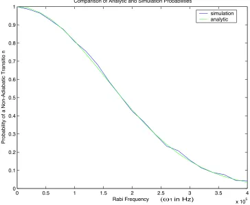
As an additional test of the numerical method, we use it to solve the differential system for the two level atom and then compare it to the analytic solution. As part of this process, we have not made the assumption of constant velocity through the crossing in the numerics, in order to test this approximation with a real system. The results of this test are seen in figure 3.4, showing an agreement with the analytic solution to within 1%. The 1% error is simply introduced by an estimate in obtaining the data points, as atoms exit the interaction region with a small oscillation in their probabilities, as seen in figure 3.5. This oscillation converges to a single probability over time (the midpoint of the peak-to-peak amplitude), but the simulation can only capture a finite range of the motion, so we must estimate this midpoint by zooming in on the plot. This small amount of error remains in the results for the different atoms.

(29)

§3.6 Numerical Results 19

0 0.5 1 1.5 2 2.5 3 3.5 4

x 105 0

0.1 0.2 0.3 0.4 0.5 0.6 0.7 0.8 0.9 1

Comparison of Analytic and Simulation Probabilities

Rabi Frequency

Probability of a Non-Adiabatic Transitio

n

simulation analytic

[image:29.595.130.494.122.420.2]

(ω1 in Hz)

Figure 3.4: Comparison of the two level atom analytic and numeric solutions. The plot is non-adiabatic transition probability as a function of Rabi frequency, and the two solutions agree to within 1%.

second over the space of tenths of millimetres. The length of a crossing is extremely small, on the order of a few microns. Any error introduced from this approximation is negligible compared to the estimation error in taking down the data. Despite this, 1% error is very small and this shows that our results for the 3 & 5 level systems will also have no more than 1% error. We ensure this by carefully monitoring the time step error, keeping the computational rounding error to the same level as for this test by increasing the number of iterations.

3.6 Numerical Results

The numerical simulations were run a number of times each in order to build up probability plots as the Rabi frequency is varied. Looking at figure 3.6, the result for the 3 level atom, we can see that an atom starting in the_|0_istate is coupled into the_|1_iand_{| −}1_istates in equal probability, regardless of Rabi frequency. This is simply due to the symmetry in the coupled set of equations, and is an important result, showing that you can never select to spin flip only into one of the | ±1_i states if starting in the_|0_i state.

(30)

0.01020 0.0103 0.0104 0.0105 0.0106 0.0107 0.0108 0.0109 0.011 0.0111 0.1

0.2 0.3 0.4 0.5 0.6 0.7 0.8 0.9 1

Three Level Atom at 200Khz

Time

Probability

[image:30.595.96.467.99.414.2]

0 state 1 & -1 states

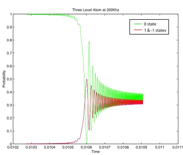
Figure 3.5: An example of one of the simulations for the three level atom. The atom enters in the|0istate, and exits the avoided crossing region with an oscillation in its probabilities retained. An atoms probability of being in a given state takes longer to settle down into a definite value after exiting the crossing, since the system is essentially a harmonic oscillator suffering a brief perturbation from the applied RF field. This is not an artefact of the numerics, but rather an interesting part of the dynamics, and a small source of error in the final numerical results.

high Rabi frequency, the atom just passes through the crossing with no resultant spin flip, just as if there were no applied RF field. This is interesting, giving us a frequency range for the atomic waveplate of 0< ω1<400KHz, outside of which no spin flips occur.

Figure 3.7 shows the results for the five level system. We can see the similar dynamics as the three level system, with the _{| ±}2_i states always evident in equal probabilities, as well as the _{| ±}1_i states equal in probability. Apart from exhibiting these same important dynamics as the three level atom, the additional two levels in this system add an extra effect. As the Rabi frequency increases towards the adiabatic following limit, the_|±2_istates disappear in probability first, reducing the possible exit states to the same set as the three level system (if we ignore the difference in F number). After this, we can see the adiabatic following of the_|0_i state take form in the same way as the 3 level system, all of which is expected due to the symmetry in their avoided crossing structure.

3.7 Conclusion

(31)

§3.7 Conclusion 21

[image:31.595.125.492.125.428.2]

(ω1 in Hz)

Figure 3.6: The three level atom numerical results. The plot is non-adiabatic transition probability as a function of Rabi frequency, for a fixed position of the crossing.

(32)

[image:32.595.102.461.276.573.2]

(ω1 in Hz)

(33)

Chapter 4

5 Level Atom Wavepacket Dynamics

4.1 Overview of this chapter

In this chapter we consider the atomic waveplate with real atomic pulses. We model the behaviour of a matter wave packet from an atom laser, as it crosses the RF resonance. This is done using a numerical one dimensional semi-classical model.

4.2 Atomic Wave Packets

Up until this point, we have considered our atomic beams as atoms falling under gravity, following a classical trajectory. This is not the case, however, for a real atom laser beam. The atoms are in the ground state of the trap, behaving as matter waves, each with a spatial extent. Atoms are outcoupled in either a pulsed or continuous manner, and each pulse is composed of many atoms all acting in a coherent manner; a wavepacket rather than a collection of classical particles. It is important to know how these wavepackets will behave when interacting with the waveplate field. In this section we perform an investigation of how a matter wave packet will behave as it passes through the RF field.

BEC

Gravity 1.1mm

[image:33.595.227.396.513.696.2]

Atomic Pulse

Figure 4.1: A pulsed atom laser. Atomic pulses outcoupled from the condensate are essentially small copies of the condensate; each a wavepacket whose evolution can be described through the GP formalism

In order to gain an understanding of the behaviour of these wavepackets in the RF resonance from our waveplate, we consider the case of a single pulse of atoms emitted from an atom laser.

(34)

[image:34.595.154.411.592.676.2]

24 5 Level Atom Wavepacket Dynamics

Figure 4.1 shows a pulsed atom laser created in the ANU laboratory by Nick Robins [18]. We can see the spatial extent of the pulses quite clearly, with each pulse containing approximately 104 atoms from a condensate of about 105 atoms. A single pulse is effectively a small copy of the BEC from which it has been outcoupled into the _|0_i state by an RF induced spin transition.

4.3 Five Level Atom in the 1-D GP Formalism

Our investigation starts with an analysis of the dynamics, which are described quite differently to those of the single atom. We consider our system in the F = 2 state of rubidium, a pulse of atoms from the ANU atom laser. Each pulse from this laser can be described as a Gaussian wavepacket within the mean field approximation. Within this approximation, the atomic cloud is described by a single wavefunction obeying different time evolution from that described by the Schr¨odinger equation. The time evolution of a wavepacket is instead described by the famous Gross-Pitaevski (GP) equation [19]

i¯h∂ψ(~r, t)

∂t = −

¯

h2

2m∇

2₊_V₍_~r_{) +}_U

0|ψ(~r, t)|2

!

ψ(~r, t) (4.1)

where U0|ψ(~r, t)|2 is the total density potential interaction term. This equation is a non-linear version of the Schdinger equation, and in general is not solvable analytically. Because of this, we move straight to a numerical solution for the dynamics after first setting up the differential equations that will govern the behaviour. The dynamics we are interested in occur in the z direction, so we use the one dimensional GP formalism for simplicity.

Now, for our system we must include the electronic behaviour, so the time evolution of our system is described by this equation

i¯h∂ψ(~z, t)

∂t =

ˆ

Hgp+ ˆHE

ψ(~z, t) (4.2)

where we have defined the system hamiltonian as the sum of two parts. The first term, ˆHgp, is just the GP equation hamiltonian, and the second is the electronic interaction part. We can easily define the electronic part of the hamiltonian, since this is just the interaction of the rubidium valence electron with the magnetic fields. This interaction with the trap field and the applied RF field has already been defined for our 5 level atom in the last chapter as

ˆ

HE = ¯h

         

2∆(z) ω1

2 0 0 0

ω1

2 ∆(z)

q

3

8ω1 0 0

0 q3₈ω1 0

q

3

8ω1 0 0 0 q3₈ω1 −∆(z) ω₂1

0 0 0 ω1

2 −2∆(z)

          (4.3)

within an interaction picture, and with the rotating wave approximation already made. Now, our general state is given by

|ψ(z, t)_i=X m

Cm(z, t)eiksz

|m_i (4.4)

(35)

§4.4 The 1-D Simulation 25

issues as for the other simulations, namely that the atoms are uninteresting for most of their fall, and that the simulation must be run in a reasonable time.

This general state is then substituted into our GP equation, producing a set of coupled differential equations that we numerically integrate.

4.4 The 1-D Simulation

The initial starting conditions for the simulation were given by the same resonance position and magnetic trap parameters as for the previous simulations, with the addition of the normalised gaussian pulse. The pulse’s initial density and FWHM were taken from observational measure-ments of the atom laser pulses taken by Nick Robins [18].

With initial tests of the code, an estimate of the execution time was found to be on the order of several days on the super computer. This is despite minimising the range of the simulation to only one full pulse width on either side of the crossing for one of the tests. We find that fully realistic parameters for the simulation are just too large for it to be done properly in the time available.

With this in mind the simulation parameters were adjusted in order to perform the simulation within a reasonable time. With our grid size restricted by this requirement, we have to take drastic measures to ensure that the real and momentum space wavefunctions stay inside the grid. Gravity is halved, and the magnetic trap gradient reduced so that the detuning term in the hamiltonian, ¯h∆(z) = ¯hα(z₋zc), is the same as the reduced gravitational potential. This gives α = 6.54_×109_{, where this is proportional to the trap field gradient as seen previously.} Both of these changes have to be done, since the_|0_i state is dependent upon gravity alone, and the other states’ dynamics depend upon the combination of the potentials. Although reducing gravity is not possible in reality, the same effect is achieved if we consider the outcoupled atoms as propagating within a tilted waveguide [20]. Since gravity is halved, the angle of this waveguide from the horizontal would have to be 30 degrees.

The Rabi frequency, ω1, was chosen by looking at the previous classical motion simulation results for the five level atom. This was kept to a small value of 40kHz that results in a moderate amount of beamsplitting for the classical motion case. This is, however, quite a large value for this system with the reduced potentials involved, and transfers the atoms into other states quite strongly. The simulation is now one showing the behaviour of a pulse crossing the resonance within a heavily reduced trap potential.

Our starting state for the pulse is one containing 4_×104atoms within a gaussian shape with a FWHM of 30µmin space. The position of the crossing is at a distance of 0.5mm from the centre of the magnetic trap and is fractionally closer to the centre than for the previous simulations. This was done simply to reduce the initial momentum of the pulse as an extra measure to keep the momentum space wavefunction within the simulation grid. The pulses starting position was defined by setting the centre of the pulse at 0.44mm from the trap centre. The simulation was run for 1.2ms with the spatial range of 3mm, starting from 0.35mm and finishing at 0.65mm.

4.5 GP Simulation Results

(36)

atoms have been transferred almost equally into the _{| ±}2_i states, and nearly all of the rest into the_|0_istate. Only a miniscule amount of atoms remains in the_{| ±}1_i states, appearing as almost zero in figure 4.2.

0 0.2 0.4 0.6 0.8 1 1.2 1.4

x 10 3

0 0.5 1 1.5 2 2.5 3 3.5

4x 10

4

Time (s)

Number of Atoms

[image:36.595.138.429.172.411.2]

0 state 1 state -1 state 2 state -2 state

Figure 4.2: Plot of the atomic number against the time. The centre of the resonance region lies at approximately t = 0.5ms. Atoms are coupled into the | ±1istates during the time the pulse traverses the resonance. As the atom exits the resonance the number in each state finalises

Looking much closer at the plot, as seen in figure 4.3, we can see a small difference in the atomic number between the _|+ 1_i state and the _{| −}1_i state. Similarly, there is a small number difference between the _|+ 2_i state and the _{| −}2_i state. This is different to the dynamics for the five level atom in the classical trajectory simulations, where the probability of atoms in the |+ 1_i state was the same as the _{| −}1_i state (this also holds for the_|+ 2_i state and the _{| −}2_i state). This difference in atomic number for these states is simply caused by the asymmetry in the potential introduced by use of the GP Hamiltonian, and is not a computational error as the number of atoms is conserved. This asymmetry in the potential breaks the symmetry of the differential equations that exists in the Landau-Zener analysis of the F = 2 (and F = 3) atom, causing the differences in atomic number for the states due to the different coupling.

(37)

§4.5 GP Simulation Results 27

Time (s)

Number of Atoms

[image:37.595.177.449.110.334.2]

1 state -1 state 2 state -2 state

Figure 4.3: A closer look at the atomic number against the time. We have added 1.3∗104

to the| ±1i

states, in order to fit them on the one plot. There is a small difference in the atomic number between the

|+ 1istate and the| −1istate. There is also a small number difference between the|+ 2istate and the

| −2istate.

Now we look at the spatial behaviour of the wavepacket. This is shown in figure 4.5 a), where we can see the entire pulse falling under gravity. As it passes through the resonance, it loses its nice regular gaussian shape, spreading out in space and breaking up slightly, but continuing to fall under gravity (It is difficult to see this in any printed picture, but is evident within the full screen plotting environment within Matlab). This behaviour is interesting, since the majority of the atoms have been transferred into the trapped and anti-trapped _{| ±}2_i states. Our RF resonance has simply changed the polarisation state of the atomic pulse without breaking it up by a large amount.

The pulse should break up into separate parts, and we can see evidence of this in the shape at the end of the simulation. What has happened is that the existing kinetic energy of atoms when they hit the resonance is in excess of the potential energy imparted from the interaction with the magnetic trap, for atoms in the trapped and anti-trapped states. What this shows us is the importance of balancing the magnetic trap gradient against gravity. In order for us to see the beamsplitting effect of the RF field in a spatial plot, the spatial detuning term, ¯h∆(z), must be an order of magnitude larger than the gravitational potential. This would, however, increase the simulation time enormously, as previously mentioned.

A series of momentum space plots show the simulation more clearly. Figure 4.5 b) is a momentum density plot for the _|0_i state, showing the atoms in it falling under gravity, with positive increasing momentum. The density of the state diminishes with the encounter with the avoided crossing, as atoms are coupled to the other states.

(38)

0.01250 0.013 0.0135 0.014 0.0145 0.015 0.0155 0.016 0.1

0.2 0.3 0.4 0.5 0.6 0.7 0.8 0.9 1

Probability

Time (s)

[image:38.595.96.466.87.410.2]

2 & -2 states 1 & - 1 states 0 state

Figure 4.4: The five level atom simulation for a classical trajectory (Landau-Zener analysis). The crossing position, trap gradient, gravity, and the Rabi frequency have all been adjusted to coincide with the GP simulation parameters. Zooming in on the plot in Matlab, we can see that the final probability for the

|0istate is 0.025. The probabilities for the| ±2istates are equal at 0.225, as are the probabilities for the

| ±1istates, at 0.2625.

is also as we expect, clearly being accelerated away from the trap centre faster than the simple free fall of the_|0_istate. This is the source of the break up in the pulse regularity after it has hit the resonance, and the large spread of the momentum shows extra behaviour that we will look at later.

Figures 4.7 shows the momentum space for the _{| ±}1_i states. The densities of these states increase and decrease with the atomic coupling, as we have seen before in figure 4.2. What is interesting is that the majority of the atoms in these states do not accelerate across the grid any faster than the falling _|0_i state atoms. This means that most of the atoms fall under gravity, instead of fighting it or accelerating faster than it. There is a simple explanation for this. Looking at the hamiltonian for the system, we see the potential that atoms in the _{| ±}1_i states feel is just the sum of two terms, M g(z₋zc)±¯h∆(z). These two terms have been balanced out, being equal in magnitude, so atoms in these states are experience no potential and are just carried by their initial momentum. Similarly, if we look at the potential terms for the _{| ±}2_istates, we can see that the total potential they feel is just M g(z₋zc)±2¯h∆(z). Because of the magnitude of these terms, atoms in the _{| ±}2_i states experience a potential of just _±¯h∆(z), and this explains the small amount of beamsplitting that is visible.

(39)

§4.6 Conclusion 29

of these momentum space plots as shown in figure 4.8. This plot shows the momentum space plots for the _{| ±}1_i and _{| ±}2_i states, where we have added in a green line (slightly offset from the data) to show the_|0_i momentum. We can see quite clearly how most of the_{| ±}1_i states just fall under gravity, but that a small fraction of the_{| ±}1_i state atoms are behaving as if ‘dragged’ by the _{| ±}2_i states. The momentum spread of the_{| ±}2_i states can be seen better, showing how the atoms are all accelerated by varied amounts from the trapping potential interaction. This is most likely due to interparticle interactions, since the atoms in the leading edge of the pulse are coupled into other states first. As they are accelerated from the beamsplitter, they may very well interact with atoms still in the_|0_i or_{| ±}1_istates that haven’t finished crossing the resonance.

4.6 Conclusion

We have carried out a difficult simulation for an atomic wavepacket crossing the RF resonance. This gives us an idea of how an atomic wavepacket behaves when crossing our waveplate field. The wavepacket will simply break up, but with a large momentum spread in its final states. The magnetic trap field was found to be crucial to the beamsplitting dynamics, with a low gradient field unable to split the atomic pulse by a great deal. For a low gradient trap field, the atomic waveplate simply changes the polarisation of an atomic beam, without splitting it.

(40)

a)

[image:40.595.61.583.180.594.2]

b)

(41)

§4.6 Conclusion 31

a)

[image:41.595.89.577.197.592.2]

b)

(42)

a)

[image:42.595.59.571.197.603.2]

b)

(43)

§4.6 Conclusion 33

Ti

m

e

Ti

m

e

Ti

m

e

Ti

m

e

Momentum

a)

b)

d)

c)

-1 State

-2 State

1 State

[image:43.595.86.594.189.606.2]

2 State

(44)

(45)

Chapter 5

Designing The Atomic Waveplate

5.1 Overview of this chapter

In this chapter, we consider the design of the RF coil for the atomic waveplate experiment, building on the knowledge obtained from the numerical models. Once the coil has been optimised, we look at the power required to drive the circuit. The current required is found to exceed that provided by a standard power supply, and so a tuned circuit is designed for the experiment.

5.2 A look at the experimental set up

As discussed in the introduction, the experimental setup for the atomic waveplate consists of an RF field applied perpendicular to the magnetic trap field. A simplified picture of the experimental set up is shown in figure 5.1, with the waveplate coil mounted below the magnetic trap coils. The main thing to note is the orientation of the applied coil. We define its axial direction as the x

direction for our experiment, perpendicular to the z direction, in which the atom falls and feels the trap field. The distance from the coil to the falling atomic pulse is small, no less than 20mm. This means we are operating in the long wavelength regime, where the RF wavelength is much greater than both the distance to the falling atoms and the coil radius; so our atoms experience a uniform field in the x direction.

In designing the atomic waveplate, we want to create an RF coil that has an easily variable magnetic field. We wish to have a coil where all that we need to do is vary the input voltage to perform a different waveplate experiment. For the purposes of the initial design, however, we will consider performing a beamsplitting experiment upon atoms in the F = 2 state.

We use the five level atom Landau-Zener model, looking at figure 3.7, and can see that a Rabi frequency of ω1 = 200kHz will transfer the |0i state almost entirely into the other states. Since ω1 = 1_¯_hgfµbB1, this corresponds to a B field amplitude of 4.4×10−6T. We use the same parameters here as those in the numerical models, with the RF resonance region at

zc = 0.55×10−3, and using the relation derived for this as a function of applied RF frequency,

zc = ω−ω0(z= 0)

α (5.1)

we find that we need to drive the circuit atf = _2πω = 8.65M Hz, or 54.35MHz in angular frequency units.

From our experience with a full wavepacket in the last chapter, however, we can only know that these parameters will provide a strong beamsplitting effect. We will not know exactly in what percentage the_|±1_iand_|±2_istates will be occupied when a pulse hits the resonance. This will have to be investigated with a larger numerical GP model before carrying out the simulation.

The atomic waveplate