promoting access to White Rose research papers
White Rose Research Online
Universities of Leeds, Sheffield and York
http://eprints.whiterose.ac.uk/
This is an author produced version of a paper published in Journal of Computational and Applied Mathematics.
White Rose Research Online URL for this paper:
Published paper
Winkler, J.R., Hasan, M. (2010) A non-linear structure preserving matrix method for the low rank approximation of the Sylvester resultant matrix, Journal of Computational and Applied Mathematics, 234 (12), pp. 3226-3242
A non-linear structure preserving matrix
method for the low rank approximation of the
Sylvester resultant matrix
Joab R. Winkler,
aMadina Hasan
aaDepartment of Computer Science, The University of Sheffield, Regent Court,
211 Portobello Street, Sheffield S1 4DP, United Kingdom
[email protected], [email protected]
Abstract
A non-linear structure preserving matrix method for the computation of a struc-tured low rank approximation S( ˜f ,˜g) of the Sylvester resultant matrix S(f, g) of two inexact polynomials f = f(y) and g = g(y) is considered in this paper. It is shown that considerably improved results are obtained when f(y) and g(y) are processed prior to the computation of S( ˜f ,˜g), and that these preprocessing op-erations introduce two parameters. These parameters can either be held constant during the computation ofS( ˜f ,˜g), which leads to a linear structure preserving ma-trix method, or they can be incremented during the computation ofS( ˜f ,g˜), which leads to a linear structure preserving matrix method. It is shown that the non-linear method yields a better structured low rank approximation ofS(f, g) and that the assignment off(y) andg(y) is important becauseS( ˜f ,˜g) may be a good struc-tured low rank approximation of S(f, g), butS(˜g,f˜) may be a poor structured low rank approximation ofS(g, f) because its numerical rank is not defined. Examples that illustrate the differences between the linear and non-linear structure preserving matrix methods, and the importance of the assignment off(y) andg(y), are shown.
Key words: Sylvester matrix, structured low rank approximation
1 Introduction
In particular, a resultant matrix, the entries of which are functions of the coefficients of the polynomials, is singular if and only if the curves intersect. Although design intent may require that the curves intersect, inexact data may imply they do not intersect, in which case the design intent is realised by perturbing the coefficients of the polynomials slightly such that their resultant matrix becomes singular, that is, a structured low rank approximation of the given resultant matrix is required. This paper compares the methods of struc-tured total least norm (STLN) [13] and strucstruc-tured non-linear total least norm (SNTLN) [14] for the calculation of a structured low rank approximation of the Sylvester resultant matrix, which is one type of resultant matrix.
The Sylvester resultant matrix S(f, g) ∈ R(m+n)×(m+n) of the polynomials f =f(y) and g =g(y),
f(y) =
m
X
i=0
aiym−i and g(y) = n
X
i=0
biyn−i, a0, b0 6= 0, (1)
is
S(f, g) =
a0 b0
a1 . .. b1 . ..
..
. . .. a0 ... . .. b0 am−1 . .. a1 bn−1 . .. b1 am . .. ... bn . .. ...
. .. am−1 . .. bn−1
am bn
, (2)
where the coefficientsai off(y) occupy the firstncolumns and the coefficients
bi of g(y) occupy the last m columns.
The calculation of a structured low rank approximation of S(f, g) is closely related to the calculation of an approximate greatest common divisor (AGCD) off(y) andg(y). For example, Bini and Boito [1] discuss three methods, based on the structure of the SylvesterS(f, g) and B´ezoutB(f, g) resultant matrices, for AGCD computations. The QR decomposition ofS(f, g) is used by Corless
et. al. [3], and Zarowski et. al. [18], and the singular value decomposition of
and Pad´e approximations are used by Pan [11].
Many methods for the calculation of an AGCD of two inexact polynomials involve two stages. In particular, the degree of an AGCD of the polynomials is determined initially, after which the coefficients of the AGCD are calculated. The computation of the degree of an AGCD of f(y) and g(y) is equivalent to the determination of the rank loss of a resultant matrix, and methods for this computation are considered in [17]. It is assumed in this paper, however, that the degree of an AGCD is known. This assumption is also made in [8,10,15,16], and a linear structure preserving method is used in these references to compute a structured low rank approximation of S(f, g).
If the ratio of the maximum coefficient (in magnitude) to the minimum co-efficient (in magnitude) of {f(y), g(y)} is large, the polynomials must be processed before a structured low rank approximation S( ˜f ,g˜) of S(f, g) is computed. These preprocessing operations introduce two parameters, which can either be held constant, or incremented, during the computation ofS( ˜f ,g˜). A linear structure preserving matrix method is used if they are held constant, but a non-linear structure preserving matrix method is required if they are incremented. Considerably improved results are obtained when the preprocess-ing operations are included in the computation of S( ˜f ,g˜), and the non-linear method yields better results than the linear method because the numerical rank of S( ˜f,g˜) is, in general, more clearly defined. Furthermore, it is shown that the assignment of the polynomials tof(y) andg(y) is important because the numerical rank of a structured low rank approximation ofS(f, g) may be defined, but the numerical rank of a structured low rank approximation of
S(g, f) may not be defined.
Subresultant matrices, which are derived from S(f, g) and are important for the calculation of S( ˜f ,g˜), are discussed in Section 2, and the preprocessing operations on f(y) andg(y) are considered in Section 3. Section 4 contains a brief comparison of STLN and SNTLN, and the application of SNTLN to the computation ofS( ˜f ,˜g) is discussed in Section 5. Section 6 contains examples that show the differences in the results using STLN and SNTLN, and the importance of the polynomial order, (f, g) or (g, f), for the computation of a structured low rank approximation of the Sylvester matrix of f(y) and g(y). A summary of the paper is contained in Section 7.
2 Subresultant matrices
product of two polynomials as a matrix-vector product.
If ˆf(y) and ˆg(y) are the theoretically exact forms off(y) andg(y) respectively, and the degree of their greatest common divisor (GCD) is ˆd, then there exist quotient polynomialsuk(y) andvk(y), and a common divisor polynomialdk(y),
such that fork = 1, . . . ,dˆ,
dk(y) =
ˆ
f(y)
uk(y)
= gˆ(y)
vk(y)
, degvk <deg ˆg =n, deguk <deg ˆf =m, (3)
where
uk(y) = m−k
X
i=0
uk,iym−k−i and vk(y) = n−k
X
i=0
vk,iyn−k−i.
It follows from (3) that there exists a non-zero polynomial tk(y) such that
tk(y) =vk(y) ˆf(y) = uk(y)ˆg(y), k = 1, . . . ,d,ˆ
and if tk ∈Rm+n−k+1 is the vector of coefficients oftk(y), then
tk=Ck( ˆf)vk =Dk(ˆg)uk, (4)
where Ck( ˆf)∈R(m+n−k+1)×(n−k+1), Dk(ˆg) ∈R(m+n−k+1)×(m−k+1), and uk and
vkare the vectors of coefficients ofuk(y) andvk(y) respectively. It follows from
(4) that
Ck Dk
vk
−uk
=Sk
vk
−uk
= 0, k = 1, . . . ,
ˆ
d, (5)
where Ck = Ck( ˆf), Dk =Dk(ˆg), Sk =Sk( ˆf ,gˆ) ∈ R(m+n−k+1)×(m+n−2k+2) and
S1( ˆf ,gˆ) =S( ˆf,gˆ). The matrixSk( ˆf ,gˆ) is the kth subresultant matrix, which
is formed by deleting the last (k−1) rows ofS( ˆf ,ˆg), the last (k−1) columns of C1( ˆf), and the last (k−1) columns ofD1(ˆg).
The polynomials ˆf(y) and ˆg(y) have common divisors of degrees 1,2, . . . ,d,ˆ
because the degree of their GCD is ˆd, but they do not have a common divisor of degree ˆd+ 1, and thus
rankSk( ˆf,gˆ)< m+n−2k+ 2, k = 1, . . . ,dˆ
It follows that (5) can be transformed, for k = 1, . . . ,dˆ, from a homogeneous equation to a linear algebraic equation by setting vk,0 = −1, that is, the
coefficient of yn−k is set equal to −1. Equation (5) therefore becomes
Akx=ck, k= 1, . . . ,d,ˆ (6)
where ck ∈ Rm+n−k+1 is the first column of Sk, Ak ∈ R(m+n−k+1)×(m+n−2k+1)
is formed from the remaining m+n−2k+ 1 columns of Sk,
Sk=
ck
Ak
, (7)
and
x=
vk,1 · · · vk,n−k −uk,0 · · · −uk,m−k
T
∈Rm+n−2k+1.
Equation (6) has an infinite number of solutions fork = 1, . . . ,dˆ−1, exactly one solution for k = ˆd, and no solution for k = ˆd+ 1, . . . ,min(m, n). Also, the homogeneous equation (5) is transformed to the linear algebraic equation (6) by the substitution vk,0 = −1, but it is easily seen that uk(y) and vk(y)
are unchanged, apart from a scalar multiplier applied to each of them, had the substitution uk,0 = 1 been made. This equivalence between the two
sub-stitutions is valid because the given polynomials ˆf(y) and ˆg(y) are exact and all computations are performed symbolically. It will be shown in Section 5.1, however, that if inexact polynomials are specified, only an AGCD can be com-puted and the choice of substitution,vk,0=−1 oruk,0 = 1, is important when
a structured low rank approximation of the Sylvester matrix of the inexact polynomials f(y) and g(y) is computed.
3 Preprocessing operations
3.1 Normalisation by the geometric mean
The Sylvester matrix S(f, g) of f(y) and g(y) is shown in (2), and its parti-tioned structure is immediately apparent. Iff(y) andg(y) are not normalised, then S(f, g) may be unbalanced if, for example, the coefficients of f(y) are significantly larger than the coefficients of g(y), in which case computational problems may occur. This problem can be overcome by normalising each poly-nomial, and normalisation by the 2-norm of the coefficients is used in [1] and [3]. In this paper, normalisation by the geometric mean of the coefficients is used because it provides a ‘better average’ when the coefficients of the polyno-mials vary over several orders of magnitude. The polynopolyno-mials (1) are therefore redefined as
f(y) =
m
X
i=0
˜
aiym−i, a˜i =
ai
Qm
j=0|aj|
m1+1
, (8)
and
g(y) =
n
X
i=0
˜
biyn−i, ˜bi =
bi
Qn
j=0|bj|
n+11
, (9)
where it is assumed that all the coefficientsaiandbi are non-zero. More
gener-ally, the geometric mean is calculated with respect to the non-zero coefficients only.
3.2 Relative scaling of the polynomials
It follows from (2) that
rankS(f, g) = rankS(f, αg), α∈R\0, (10)
which states that the GCD of two polynomials is defined up to an arbitrary scalar multiplier, GCD(f, g) ∼ GCD(f, αg). Equation (10) is not, however, satisfied when computations are performed in a floating point environment because the numerical rank of S(f, αg) is a function of α [15,16]. It follows from (8) and (9) that the parameter α can be interpreted as the weight of
It is shown in [4,5] that problems can occur in algorithms for the computation of the roots of a polynomial when the coefficients of the polynomial vary widely in magnitude. It is therefore desirable to minimise the ratio of the maximum coefficient (in magnitude) to the minimum coefficient (in magnitude), and since the coefficients off(y) andαg(y), that is, the arguments ofS(f, αg), are ˜
ai and α˜bi respectively, an optimal value α minimises the ratio
max
maxi=0,...,m|˜ai|,maxj=0,...,n
α˜bj
min
mini=0,...,m|˜ai|,minj=0,...,n
α˜bj
. (11)
This minimisation problem can be written as:
Minimise st
Subject to
t≥ |˜ai|, i= 0, . . . , m
t≥α
˜bj
, j = 0, . . . , n
s≤ |˜ai|, i= 0, . . . , m
s≤α
˜bj
, j = 0, . . . , n
s >0
α >0.
The transformations
T = logt, S = logs, µ= logα, α˜i = log|˜ai| and β˜j = log
˜bj
,
enable this constrained minimisation problem to be written as:
Minimise T −S
Subject to
T ≥ α˜i, i= 0, . . . , m
T − µ≥ β˜j, j = 0, . . . , n
−S ≥ −α˜i, i= 0, . . . , m
−S + µ≥ −β˜j, j = 0, . . . , n,
which is a linear programming problem, where the objective function is
T −S=
1 −1 0
T
S
µ
.
There are 2(m+n+ 2) constraints in the linear programming problem (12), and if a coefficient ai orbj is equal to zero, then the corresponding constraints
are deleted. The solution α0 of (12) is the optimal value of α.
The parameter α scales the coefficients of g(y) relative to the coefficients of
f(y), and it is shown in the next section that the ratio of coefficients (11) can be reduced further by scaling the independent variable y.
3.3 Scaling the independent variable
The ratio of the maximum coefficient (in magnitude) to the minimum coeffi-cient (in magnitude) of the polynomials{f(y), α0g(y)}can be reduced further
by the substitution
y=θw, (13)
wherew is the new independent variable andθ is a real constant to be deter-mined. This substitution is justified provided it does not increase the condition numbers of the roots of an arbitrary polynomial, and it is shown in [17] that this requirement is satisfied. The substitution (13) transforms the polynomials
f(y) andg(y), which are defined in (8) and (9) respectively, to
fθ(w) = m
X
i=0
˜
aiθm−i
wm−i and g
θ(w) = n
X
i=0
˜biθn−i
wn−i, (14)
and thus following (11), the optimal value θ0 of θ is the value of θ that
min-imises the ratio
maxnmaxi=0,...,m|˜aiθm−i|,maxj=0,...,n
α0˜bjθ
n−j o
minnmini=0,...,m|˜aiθm−i|,minj=0,...,n
α0˜bjθ
n−j
o . (15)
Minimise st
Subject to
t≥ |˜ai|θm−i, i= 0, . . . , m
t≥
α0˜bj
θ
n−j, j = 0, . . . , n
s≤ |˜ai|θm−i, i= 0, . . . , m
s≤
α0˜bj
θ
n−j, j = 0, . . . , n
s >0
θ >0.
The transformations
T = logt, S = logs, φ= logθ, α˜i = log|˜ai| and β˜j = log
α0˜bj
,
enable this constrained minimisation problem to be written as:
Minimise T −S
Subject to
T − (m−i)φ ≥ α˜i, i= 0, . . . , m
T − (n−j)φ ≥ β˜j, j = 0, . . . , n
−S + (m−i)φ ≥ −α˜i, i= 0, . . . , m
−S + (n−j)φ ≥ −β˜j, j = 0, . . . , n,
(16)
which is almost identical to the linear programming problem (12).
The minimisations (11) and (15) transform the polynomials (14) to
fθ0(w) = m
X
i=0
˜
aiθm0−i
wm−i and gθ0(w) = n
X
i=0
˜
biθ0n−i
wn−i,
whereθ0 is the solution of (16). The coefficients offθ0(w) andgθ0(w) define the
¯
f(w) =
m
X
i=0
a∗iθ m−i 0
wm−i and g¯(w) =
n
X
i=0
b∗iθ n−i 0
wn−i, (17)
where
a∗i =
˜
ai
Qm
j=0
˜ajθ
m−j 0
m1+1
and b∗i =
˜
bi
Qn
j=0
˜bjθ
n−j 0
n+11
,
and ˜ai and ˜bi are defined in (8) and (9) respectively. The multiplicities of the
roots of f(y) and g(y) are preserved by the transformation (13), and thus
S( ¯f,g¯) can be used to calculate an AGCD off(y) andg(y). The roots off(y) and g(y) are not, however, equal to the roots of ¯f(w) and ¯g(w), respectively, if θ0 6= 1.
Algorithm 3.1 shows the operations that are performed on the given inexact polynomials (1) before a structured low rank approximation of the Sylvester matrix S( ¯f ,g¯) is computed.
Algorithm 3.1: Preprocessing operations
Input Inexact polynomials f(y) and g(y), which are defined in (1).
Output Polynomials ¯f(w) and ¯g(w), which are defined in (17).
Begin
(1) Normalise the coefficients off(y) andg(y) by the geometric mean of their coefficients, as shown in (8) and (9).
(2) Solve the linear programming problem (12) in order to computeα0.
(3) Solve the linear programming problem (16) in order to computeθ0.
(4) Calculate the coefficients a∗
iθm0−i and b∗iθ0n−i of ¯f(w) and ¯g(w),
respec-tively.
End
4 Structured matrix methods
low rank approximation of S( ¯f,¯g) requires the determination of a Sylvester matrix S(δf, δ¯ ¯g) such that
S( ¯f+δf,¯ ¯g+δg¯) =S( ¯f,g¯) +S(δf , δ¯ g¯),
is rank deficient, where δf¯=δf¯(w) andδ¯g =δ¯g(w) are perturbation polyno-mials that are added to ¯f(w) and ¯g(w), respectively, in order to induce rank de-ficiency inS( ¯f+δf ,¯ ¯g+δg¯). The structured nature of the Sylvester matrix im-plies that structured matrix methods can be used to computeS( ¯f+δf,¯ ¯g+δ¯g), and this computation can be achieved by STLN, which preserves the affine structure ofS( ¯f,¯g), or SNTLN, which preserves the structure ofS( ¯f ,¯g) when its elements are differentiable non-linear functions of one or more parameters. These methods are considered in Sections 4.1 and 4.2 respectively.
4.1 Linear structure preserving matrix method
The method of STLN assumes thatα0 and θ0 are constant, and thus they are
not updated in the iterative scheme for the computation of the coefficients of
δf¯(w) and δg¯(w). The polynomials (17) are therefore written as
¯
f(w) =
m
X
i=0
¯
aiwm−i and ¯g(w) = n
X
i=0
¯
biwn−i, (18)
whose coefficients are
¯
ai =a∗iθ0m−i =
˜
aiθ0m−i
Qm
j=0
˜ajθ
m−j 0
m1+1
, (19)
and
¯bi =b∗
iθ n−i
0 =
˜
biθ0n−i
Qn
j=0
˜bjθ
n−j 0
n1+1
. (20)
The method of STLN allows a structured low rank approximation ofS( ¯f, α0¯g)
to be computed, where ¯f(w) and ¯g(w), and their coefficients, are defined in (18) and (19,20), respectively, and only these coefficients are updated in the iterative scheme for the computation of the coefficients of δf¯(w) and δg¯(w). In particular, α0 and θ0 are constant, and only the coefficients ¯ai and ¯bi are
4.2 Non-linear structure preserving matrix method
This method is more complex than the linear structure preserving matrix method because more parameters are updated in the iterative scheme for the computation of the coefficients of δf¯(w) and δ¯g(w). In particular, the initial values of α and θ in this scheme are α0 and θ0, that is, the solutions of the
linear programming problems (12) and (16) respectively, and the polynomials (17) are written as
¯
f(w)≈
m
X
i=0
¯
aiθm−i
wm−i and ¯g(w)≈ n
X
i=0
¯biθn−i
wn−i, (21)
where
¯
ai =a∗i =
˜
ai
Qm
j=0
˜ajθ
m−j 0
m1+1
, (22)
and
¯bi =b∗
i =
˜bi
Qn
j=0
˜bjθ
n−j 0
n+11
. (23)
The constant θ0 is retained in the denominators of these expressions for ¯ai
and ¯bi because it simplifies the update procedure for θ between successive
iterations.
The differences between the polynomials (18) and (21) are important:
• Only the coefficients ¯ai and ¯bi, which are defined in (19) and (20)
respec-tively, are updated when STLN is used.
• The coefficients ¯aiθm−i and ¯biθn−i, where ¯ai and ¯bi are defined in (22) and
(23) respectively, and α are updated when SNTLN is used.
The next section considers the method of SNTLN for the calculation of a structured low rank approximation of S( ¯f, α¯g).
5 The method of SNTLN
in (21) and the inclusion ofαfollows from (10). The Sylvester matrixS( ¯f, α¯g) of ¯f(w) and αg¯(w) is
¯
a0θm α¯b0θn
¯
a1θm−1 . .. α¯b1θn−1 . ..
... . .. ¯a0θm ... . .. α¯b0θn
¯
am−1θ . .. ¯a1θm−1 α¯bn−1θ . .. α¯b1θn−1
¯
am . .. ... α¯bn . .. ...
. .. ¯am−1θ . .. α¯bn−1θ
¯
am α¯bn
,
where ¯ai and ¯bi are defined in (22) and (23) respectively, and the optimal
values of α and θ are determined using an iterative scheme for which α0 and θ0 are the initial values. The subresultant matrixSk =Sk( ¯f , α¯g) is partitioned
as, following (7),
Sk=
ck Ak = ck
coeffs. of ¯f(w)
coeffs. of αg¯(w)
,
where ck =ck(θ)∈Rm+n−k+1 and Ak=Ak(α, θ)∈R(m+n−k+1)×(m+n−2k+1).
The polynomials ¯f(w) and ¯g(w) are inexact and they are therefore perturbed in order to induce a non-constant common divisor in their perturbed forms. If the perturbations of the coefficients of ¯f(w) and αg¯(w) are, respectively,
ziθm−i, i= 0, . . . , m and αzm+1+iθn−i, i= 0, . . . , n,
then the Sylvester matrix Bk = Bk(α, θ, z) ∈ R(m+n−k+1)×(m+n−2k+2) of the
perturbations is
Bk =
hk Ek =
z0θm αzm+1θn
z1θm−1 . .. αzm+2θn−1 . ..
..
. . .. z0θm ... . .. αzm+1θn zm−1θ . .. z1θm−1 αzm+nθ . .. αzm+2θn−1
zm . .. ... αzm+n+1 . .. ...
. .. zm−1θ . .. αzm+nθ
zm αzm+n+1
where hk=hk(θ, z)∈Rm+n−k+1 is the first column of Bk,
z =
z0 z1 · · · zm+n zm+n+1
T
∈Rm+n+2,
and Ek =Ek(α, θ, z)∈R(m+n−k+1)×(m+n−2k+1). The application of SNTLN to
the computation of an AGCD of ¯f(w) and ¯g(w) requires that the equation
(Ak(α, θ) +Ek(α, θ, z))x=ck(θ) +hk(θ, z), x∈Rm+n−2k+1,
which is the perturbed form of (6), be considered. The residual that is associ-ated with an approximate solution of this non-linear equation is
r(α, θ, x, z) =ck(θ) +hk(θ, z)−(Ak(α, θ) +Ek(α, θ, z))x, (24)
and thus if ˜r is defined as
˜
r:=r(α+δα, θ+δθ, x+δx, z+δz),
then
˜
r=ck(θ+δθ) +hk(θ+δθ, z+δz)
−
Ak(α+δα, θ+δθ) +Ek(α+δα, θ+δθ, z+δz)
(x+δx)
=ck+
∂ck
∂θ δθ+hk+ ∂hk
∂θ δθ+
m+n+1
X
i=0 ∂hk
∂zi
δzi−Akx−Akδx
− ∂Ak ∂α x
!
δα− ∂Ak ∂θ x
!
δθ−Ekx−Ekδx−
∂Ek
∂α x
!
δα
− ∂Ek ∂θ x
!
δθ−
m+n+1
X i=0 ∂Ek ∂zi δzi ! x,
to first order. It follows that
˜
r=r(α, θ, x, z)−
∂Ak ∂θ + ∂Ek ∂θ !
x− ∂ck ∂θ +
∂hk
∂θ
!!
δθ
−(Ak+Ek)δx−
∂Ak ∂α + ∂Ek ∂α ! x ! δα+
m+n+1
X i=0 ∂hk ∂zi δzi −
m+n+1
where expressions for the partial derivatives are easily calculated fromck, hk, Ak
and Ek.
It is readily verified that
hk =Pkz =
G 0m+1,n+1
0n−k,m+1 0n−k,n+1
z,
where Pk =Pk(θ)∈R(m+n−k+1)×(m+n+2),
G=G(θ) = diag
θm θm−1 · · · θ 1
∈R(m+1)×(m+1),
and
m+n+1
X
i=0 ∂hk
∂zi
δzi =Pkδz.
Also, there exists a matrixYk=Yk(α, θ, x)∈R(m+n−k+1)×(m+n+2) such that
Ykz =Ekx,
for all z, x, α, θ, and it therefore follows that on differentiating both sides of this equation with respect toz,
Ykδz=
δEk |α,θ:const.
x=
m+n+1
X
i=0
∂Ek
∂zi
δzi
!
x,
and thus (25) simplifies to
˜
r=r(α, θ, x, z)−
∂Ak
∂θ + ∂Ek
∂θ
!
x− ∂ck ∂θ +
∂hk
∂θ
!!
δθ
−(Ak+Ek)δx−
∂Ak
∂α + ∂Ek
∂α
!
x
!
δα−(Yk−Pk)δz. (26)
Thejth iteration in the Newton-Raphson method for the calculation ofz, x, α, θ,
Hz Hx Hα Hθ
(j)
δz δx δα δθ
(j)
=r(j), (27)
where r(j) =r(j)(α, θ, x, z),
Hz =Yk−Pk, Hx =Ak+Ek,
Hα=
∂A k ∂α + ∂Ek ∂α
x, Hθ =
∂A k ∂θ + ∂Ek ∂θ
x−∂ck
∂θ + ∂hk
∂θ
,
and the values ofz, x, α, θ at the (j + 1)th iteration are
z x α θ
(j+1)
= z x α θ
(j)
+ δz δx δα δθ
(j)
.
The initial value of z is z(0) = 0 because the given data is the inexact data,
and the initial values of αand θ areα0 and θ0, which are the solutions of (12)
and (16), respectively.
Equation (27) is of the form
Cy =q, (28)
where C∈R(m+n−k+1)×(2m+2n−2k+5), y ∈R2m+2n−2k+5, q∈Rm+n−k+1,
C =
Hz Hx Hα Hθ
(j)
, y=
δz δx δα δθ
(j)
, q=r(j). (29)
It is necessary to calculate the smallest perturbations zi such that the
perturbationszi, i= 0, . . . , m,occurs (n−k+ 1) times inBk, and each of the
perturbationszi, i=m+ 1, . . . , m+n+ 1, occurs (m−k+ 1) times inBk, it
follows that the weight matrix D∈R(m+n+2)×(m+n+2) associated withz is
D=
D1 0
0 D2
,
where D1 ∈R(m+1)×(m+1) and D2 ∈R(n+1)×(n+1) are diagonal matrices,
D1 = (n−k+ 1)Im+1 and D2 = (m−k+ 1)In+1.
Also,α occurs d= (n+ 1)×(m−k+ 1) times in Bk, and thus it is necessary
to minimise the function
Dz(j)+δz(j)−z(0)
dα(j)+δα(j)−α 0
θ(j)+δθ(j)−θ 0 =
Dz(j)+δz(j)
dα(j)+δα(j)−α 0
θ(j)+δθ(j)−θ 0
:=kEy−pk,
(30)
subject to (28), at each iteration, where E ∈ R(m+n+4)×(2m+2n−2k+5) and p ∈
Rm+n+4 are given by
E =
D 0 0 0 0 0d 0 0 0 0 1
, p=
−Dz
d(α0−α) θ0 −θ
(j)
,
andyis defined in (29). It is noted thatEis constant and not updated between iterations.
The minimisation of (30) subject to (28) is a least squares minimisation with an equality constraint (the LSE problem),
miny kEy−pk subject to Cy =q, (31)
which can be solved by the QR decomposition [6]. This LSE problem is solved at each iteration, whereC, pand q are updated between successive iterations. The initial value x0 of x in the iterative procedure for the solution of this
problem is obtained by setting θ=θ0, α=α0 and z =z(0) = 0, and thus from
x0 = arg minw kAk(α0, θ0)w−ck(θ0)k. (32)
The given data is the inexact polynomialsf(y) andg(y), and all computations are performed on the transformed polynomials ¯f(w) and ¯g(w). The computed structured low rank approximation Sylvester matrix isS( ˜f,g˜), where ˜f(w) and ˜
g(w) can be transformed back to their equivalents in the independent variable
y by the substitution w=y/θ∗, and θ∗ is the value of θ at the termination of
the iterative scheme for the solution of the LSE problem.
The convergence of the algorithm for the solution of the LSE problem has not been established, and the success or failure of the algorithm to computeS( ˜f ,˜g) is determined by an a posteriori test on the computed result. Specifically, the Sylvester matrix S( ˜f ,g˜) of the computed polynomials ˜f(w) and ˜g(w) is constructed in order to determine if it is, or is not, rank deficient.
Algorithm 5.1 shows the application of SNTLN for the calculation of a struc-tured low rank approximation of S(f, g).
Algorithm 5.1: SNTLN for a Sylvester matrix
Input Inexact polynomials f(y) and g(y), which are of degrees m and n
respectively and defined in (1), and the degree ˆd of the GCD of the exact forms off(y) and g(y).
Output A structured low rank approximation of S(f, g) of rank m+n−dˆ.
Begin
(1) Preprocess f(y) and g(y) using Algorithm 3.1. (2) Set k = ˆd.
(3) % Initialise the data
• Set z =z(0) = 0, which yields E
k = ∂E∂αk = ∂E∂θk = 0 and hk = ∂h∂θk = 0.
• Calculate Ak, Yk, Pk, ck,∂A∂αk,∂A∂θk and ∂c∂θk for θ = θ0, α = α0 and the
initial valuex0 ofx, which is defined in (32). Calculate the initial value
of q, which is equal to the residual,
r(α0, θ0, x0, z(0) = 0) =ck−Akx0,
and set the initial value of p, p= 0.
• Define the matrices C and E. (4) % The loop for the iterations
repeat
(a) Compute the QR decomposition of CT,
CT =QR=Q
R1
0
.
(b) Set w1 =R−1Tq.
(c) Partition EQ as
EQ=
E1 E2
,
whereE1 ∈R(m+n+4)×(m+n−k+1) and E2 ∈R(m+n+4)×(m+n−k+4).
(d) Compute
z1 =E2†(p−E1w1).
(e) Compute the solution
y=Q
w1
z1
.
(f) Set z :=z+δz, x:=x+δx, α:=α+δαand θ:=θ+δθ.
(g) UpdateAk,∂A∂θk,∂A∂αk, Ek,∂E∂θk,∂E∂αk, Yk, Pk, ck,∂c∂θk,hk,∂h∂θk (and
there-foreC) from α, θ, x and z. Compute the residual
r(α, θ, x, z) = (ck+hk)−(Ak+Ek)x,
and thus updateq. Update pfrom α, θ and z.
until krk(cα,θ,x,zh+hkk)k ≤10−12
End
5.1 The definition of the polynomials
The situation is more involved when computations are performed on inexact polynomials because (6) does not possess an exact solution in this situation. In particular, the results obtained from S(f, g) are not equal to the results obtained from S(g, f) because the entries of Ak and ck are dependent upon
the order in which the polynomials are specified, that is, the order (f, g) or the order (g, f). It is clear that this reversal of the order off(y) andg(y) does not change the normalisation of each polynomial by the geometric mean of its coefficients, and the solutions of the linear programming problems (12) and (16) need not be recomputed forS(g, f). In particular, it has been shown that
α0 andθ0are the optimal values ofαandθwhen the polynomial order (f, g) is
used. When the polynomial order (g, f) is used, computations are performed onS(¯g, αf¯), where 1/α0 is the initial value of α, and θ0 is the initial value of θ, when the method of SNTLN is used.
6 Examples
This section contains two examples that show the differences in the results between the methods of STLN and SNTLN, the importance of the order of assignment of the polynomials tof(y) and g(y), and the significant reduction in the ratio of the maximum coefficient (in magnitude) to the minimum coef-ficient (in magnitude) when the preprocessing operations discussed in Section 3 are implemented.
It is necessary to refer to the Sylvester matrices of several pairs of polynomials when the results of the examples are considered. The following notation is therefore used in all the examples:
• fˆ(y) and ˆg(y) are the theoretically exact polynomials, and S( ˆf,gˆ) and
S(ˆg,fˆ) are calculated by normalising each polynomial by the geometric mean of its coefficients.
• f(y) andg(y) are calculated from ˆf(y) and ˆg(y) by adding noise and normal-ising these inexact polynomials by the geometric mean of their coefficients.
• f¯(w) and ¯g(w) are the polynomials, the coefficients of which form the en-tries of the Sylvester matrix whose structured low rank approximation is computed. These polynomials and their coefficients are defined in (18) and (19,20) when STLN is used, and in (21) and (22,23) when SNTLN is used.
• f˜(w) and ˜g(w) are the polynomials that are computed by the methods of STLN and SNTLN, and thus S( ˜f, α∗g˜) and S(˜g,f/α˜ ∗) are the structured
low rank approximations of the Sylvester matrix off(y) andg(y). The value of α∗ depends on whether STLN or SNTLN is used:
· STLN: α∗ =α
0.
· SNTLN:α∗ is equal to the value ofαwhen the iterative procedure for the
Normalisation is not applied to ˜f(w) and ˜g(w).
The variation of the norm of the normalised residual rnorm,
rnorm =
r(α, θ, x, z)
kck(θ) +hk(θ, α)k
, (33)
where r(α, θ, x, z) is defined in (24), with the number of iterations required for the solution of the LSE problem (31) is considered in the examples.
It is assumed that the degrees of the polynomials are known, and thus the dimensions of the Sylvester matrix and its subresultant matrices are defined. Furthermore, the polynomials are defined by their roots, and the coefficients of each polynomial are obtained by the convolution of the linear factors defined by its roots.
Example 6.1
Consider the polynomials
ˆ
f(y) = (y−10−5)3(y−3.1×10⁻³)3(y−3.2×10⁻³)3(y−5)15, (34) ˆ
g(y) = (y−3.1×10⁻³)4(y−3.2×10⁻³)3(y+ 3.3×10⁶)10, (35)
whose Sylvester matrix is of order 41×41, and since their GCD is of degree 6, it follows that rank S( ˆf ,gˆ) = 35. Noise with a normwise signal-to-noise ratio of 108 was added to the polynomials (34) and (35), which were then
normalised, thereby yielding the polynomials f(y) andg(y).
Figure 1 shows the results obtained from STLN forα=θ = 1 and both these parameters are held constant, that is, the only preprocessing operation is the normalisation of each polynomial by the geometric mean of its coefficients. It is seen that
rankS( ˆf ,ˆg) = rank S(f, g) = rank S( ˜f,˜g) = 24,
which is incorrect. Although the normalised residual (33) at convergence is about 10−12, it is seen that a small normalised residual does not imply that
a correct structured low rank approximation of a Sylvester matrix has been computed.
0 10 20 30 40 50 −35
−30 −25 −20 −15 −10 −5 0
i
log
10
σi
/
σ1
i=24
i=35
(a)
0 20 40 60 80 100
−14 −12 −10 −8 −6 −4 −2 0
iteration
log
10
rnorm
(b)
Fig. 1. (a) The normalised singular values of the Sylvester matricesS( ˆf ,ˆg)♦;S(f, g)
2;S( ˜f ,˜g) ×, and (b) the normalised residual, for Example 6.1. The preprocessing operations, apart from normalising each polynomial by the geometric mean of its coefficients, are omitted.
0 5 10 15 20 25
−20 −10 0 10 20
i
log
10
|
ai
|
(a)
0 5 10 15 20
−20 0 20 40 60 80
i
log
10
|
bi
|
[image:23.612.97.475.35.224.2](b)
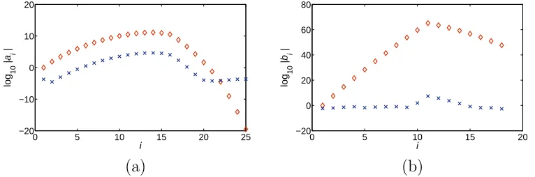
Fig. 2. The magnitude of the coefficients of (a) f(y) and (b) g(y) before, ♦, and after,×, scaling byα and θ, for Example 6.1.
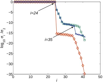
The methods of STLN and SNTLN were then used to compute structured low rank approximations ofS(f, g). Figure 3 shows the results when STLN is applied and it is seen that the computed numerical rank ofS( ˜f, α0g˜) is equal to
24, which is incorrect. Also, the results for the polynomial order (g, f), which are not shown, are unsatisfactory because the numerical rank ofS(˜g,f/α˜ 0) is
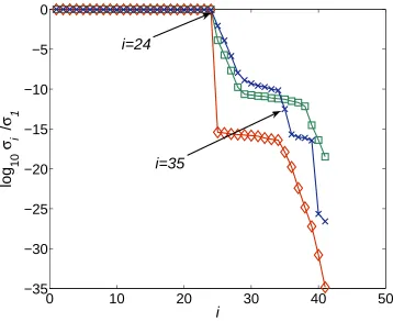
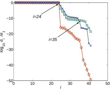
not defined. Figures 4 and 5 show the results when SNTLN is applied, and it is seen that the numerical rank of S( ˜f , α∗g˜) is not well defined because it could
be equal to either 34 or 35 (Figure 4), but the numerical rank of S(˜g,f /α˜ ∗)
has the correct value of 35 (Figure 5). These figures show that if the numerical rank is defined as the index i for which the ratio of singular values σi/σi+1 is
a maximum, then the numerical rank of S( ˜f, α∗g˜) and S(˜g,f/α˜ ∗) is equal to
39, which is incorrect.
[image:23.612.93.476.303.430.2]0
10
20
30
40
50
−35
−30
−25
−20
−15
−10
−5
0
i
log
10
σ
i/
σ
1i=24
[image:24.612.97.459.39.327.2]i=35
Fig. 3. The normalised singular values of the Sylvester matrices S( ˆf ,ˆg) ♦;S(f, g)
2; S( ˜f , α0g˜) ×, for Example 6.1. The polynomials ˜f(w) and ˜g(w) are calculated
using STLN.
STLN and SNTLN, and it is seen that the differences in the graphs are minor. Comparison of these graphs with their equivalents forS(g, f), which are shown in Figure 7, shows two significant differences:
(1) The normalised residual obtained with S(f, g) is much smaller than the normalised residual obtained with S(g, f) when STLN is used.
(2) Approximately twice the number of iterations are required to achieve convergence withS(g, f) with respect to the number of iterations required to achieve convergence withS(f, g) when SNTLN is used.
2
Example 6.2
0
10
20
30
40
50
−35
−30
−25
−20
−15
−10
−5
0
i
log
10
σ
i/
σ
1i=24
[image:25.612.98.456.37.330.2]i=35
Fig. 4. The normalised singular values of the Sylvester matrices S( ˆf ,ˆg) ♦;S(f, g)
2; S( ˜f , α∗g˜) ×, for Example 6.1. The polynomials ˜f(w) and ˜g(w) are calculated
using SNTLN. ˆ
f(y) = (y−1.8722181×10⁷)5(y−0.3124444)2
×(y−4.4199430×10⁵)7, (36)
ˆ
g(y) = (y−1.8722181×10⁷)2(y−0.3124444)6(y−8.8081342)2
×(y+ 1.6888534)7(y+ 4.5594954)9. (37)
The Sylvester matrix of these polynomials is of order 40×40 and the degree of their GCD is 4, and thus rank S( ˆf,gˆ) = 36.
Figures 8 and 9 show the results, for the polynomial orders (f, g) and (g, f) respectively, obtained from STLN when α and θ are constant and equal to one, such that the only preprocessing operation is the normalisation of each polynomial by the geometric mean of its coefficients. It is seen that
rankS( ˆf ,ˆg) = rank S(f, g) = rank S( ˜f,˜g) = 26,
and
0
10
20
30
40
50
−50
−40
−30
−20
−10
0
i
log
10
σ
i/
σ
1i=24
[image:26.612.99.457.37.330.2]i=35
Fig. 5. The normalised singular values of the Sylvester matricesS(ˆg,fˆ) ♦; S(g, f)
2; S(˜g,f /α˜ ∗) ×, for Example 6.1. The polynomials ˜f(w) and ˜g(w) are calculated using SNTLN.
0 20 40 60 80 100
−15 −10 −5 0
iteration
log
10
rnorm
(a)
0 20 40 60 80 100
−15 −10 −5 0 5
iteration
log
10
rnorm
[image:26.612.97.473.401.527.2](b)
Fig. 6. The variation of the normalised residual with the number of iterations, for Example 6.1, using (a) STLN and (b) SNTLN, forS(f, g).
all of which are incorrect, and the normalised residuals, shown in Figures 8(b) and 9(b), at convergence are equal to about 10−9 and 10−10, respectively.
This is another example that shows that a small normalised residual does not guarantee that a structured low rank approximation of a Sylvester matrix has been computed.
0 20 40 60 80 100 −8
−6 −4 −2 0
iteration
log
10
rnorm
(a)
0 20 40 60 80 100
−10 −5 0 5 10
iteration
log
10
rnorm
[image:27.612.98.474.29.151.2](b)
Fig. 7. The variation of the normalised residual with the number of iterations, for Example 6.1, using (a) STLN and (b) SNTLN, forS(g, f).
0 10 20 30 40
−45 −40 −35 −30 −25 −20 −15 −10 −5 0
i
log
10
σi
/
σ1
i=26
i=36
(a)
0 20 40 60 80 100
−10 −8 −6 −4 −2 0 2
iteration
log
10
rnorm
(b)
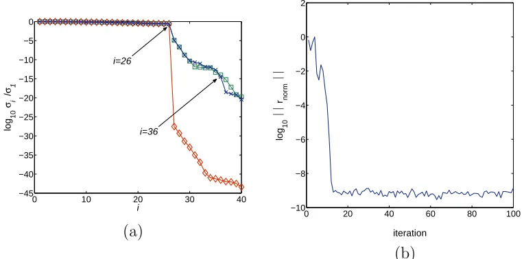
Fig. 8. (a) The normalised singular values of the Sylvester matricesS( ˆf ,ˆg)♦;S(f, g)
2;S( ˜f ,˜g) ×, and (b) the normalised residual, for Example 6.2. The preprocessing operations, apart from normalising each polynomial by the geometric mean of its coefficients, are omitted.
3.1 reduce considerably the ratio of the maximum magnitude of the coefficients to the minimum magnitude of the coefficients, for both polynomials.
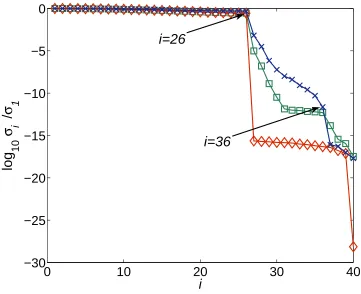
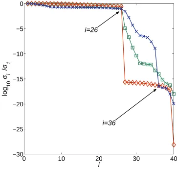
Figures 11 and 12 show the results using STLN and SNTLN, respectively, for the order (g, f). Figure 11 shows that STLN does not compute a structured low rank approximation because the numerical rank could be equal to either 26 or 36, and Figure 12 shows that SNTLN does not compute a structured low rank approximation because the computed numerical rank is equal to 35. The graphs shown in these figures are very similar to their equivalents when the order (f, g) is used.
[image:27.612.93.475.209.398.2]0 10 20 30 40 −30
−25 −20 −15 −10 −5 0
i
log
10
σi
/
σ1
i=26
i=36
(a)
0 20 40 60 80 100
−11 −10 −9 −8 −7 −6 −5 −4 −3 −2
iteration
log
10
rnorm
(b)
Fig. 9. (a) The normalised singular values of the Sylvester matricesS(ˆg,fˆ)♦;S(g, f)
2;S(˜g,f˜) ×, and (b) the normalised residual, for Example 6.2. The preprocessing operations, apart from normalising each polynomial by the geometric mean of its coefficients, are omitted.
0 5 10 15
−20 0 20 40 60 80
i
log
10
|
ai
|
(a) 0 5 10 15 20 25 30
−5 0 5 10 15 20 25
i
log
10
|
bi
|
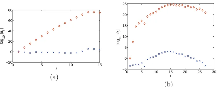
[image:28.612.96.474.32.201.2](b)
Fig. 10. The magnitude of the coefficients of (a) f(y) and (b) g(y) before, ♦, and after,×, scaling byα and θ, for Example 6.2.
convergence is the same for both methods. 2
[image:28.612.96.474.315.466.2]0
10
20
30
40
−30
−25
−20
−15
−10
−5
0
i
log
10
σ
i/
σ
1i=26
[image:29.612.96.457.37.331.2]i=36
Fig. 11. The normalised singular values of the Sylvester matricesS(ˆg,fˆ)♦;S(g, f)
2; S(˜g,f /α˜ 0) ×, for Example 6.2. The polynomials ˜f(w) and ˜g(w) are calculated
using STLN.
7 Summary and discussion
This paper has considered the use of STLN and SNTLN for the calculation of an AGCD of two inexact polynomials. The preprocessing operations discussed in Section 3 introduce the parametersαand θ, and the examples suggest they are important for the calculation of a structured low rank approximation of the Sylvester matrix of f(y) andg(y).
0
10
20
30
40
−30
−25
−20
−15
−10
−5
0
i
log
10
σ
i/
σ
1i=26
[image:30.612.94.456.43.388.2]i=36
Fig. 12. The normalised singular values of the Sylvester matricesS(ˆg,fˆ)♦;S(g, f)
2; S(˜g,f /α˜ ∗) ×, for Example 6.2. The polynomials ˜f(w) and ˜g(w) are calculated using SNTLN.
0 20 40 60 80 100
−12 −10 −8 −6 −4 −2 0
iteration
log
10
rnorm
(a)
0 20 40 60 80 100
−12 −10 −8 −6 −4 −2 0
iteration
log
10
rnorm
(b)
Fig. 13. The variation of the normalised residual with the number of iterations, for Example 6.2, using (a) STLN and (b) SNTLN, forS(g, f).
values of α, θ and z are computed by SNTLN, but only the optimal value of
[image:30.612.97.473.469.594.2]respectively, are defined by the given inexact data.
The results show it is necessary to determine the best matrix, S(f, g) or
S(g, f), to use for the computation of a structured low rank approximation of the Sylvester matrix off(y) andg(y). A criterion that enables the optimal matrix, S(f, g) or S(g, f), to be determined will improve the quality of this structured low rank approximation.
References
[1] D. A. Bini and P. Boito. Structured matrix-based methods for ǫ-gcd: Analysis and comparisons. In Proc. Int. Symp. Symbolic and Algebraic Computation, pages 9–16. ACM Press, New York, 2007.
[2] R. M. Corless, P. M. Gianni, B. M. Trager, and S. M. Watt. The singular value decomposition for polynomial systems. InProc. Int. Symp. Symbolic and Algebraic Computation, pages 195–207. ACM Press, New York, 1995.
[3] R. M. Corless, S. M. Watt, and L. Zhi. QR factoring to compute the GCD of univariate approximate polynomials. IEEE Trans. Signal Processing, 52(12):3394–3402, 2004.
[4] D. K. Dunaway.A Composite Algorithm for Finding Zeros of Real Polynomials. PhD thesis, Southern Methodist University, Texas, 1972.
[5] S. Ghaderpanah and S. Klasa. Polynomial scaling. SIAM J. Numer. Anal., 27(1):117–135, 1990.
[6] G. H. Golub and C. F. Van Loan. Matrix Computations. John Hopkins University Press, Baltimore, USA, 1996.
[7] J. T. Kajiya. Ray tracing parametric patches. Computer Graphics, 16:245–254, 1982.
[8] E. Kaltofen, Z. Yang, and L. Zhi. Structured low rank approximation of a Sylvester matrix, 2005. Preprint.
[9] N. Karmarkar and Y. N. Lakshman. Approximate polynomial greatest common divsior and nearest singular polynomials. In Proc. Int. Symp. Symbolic and Algebraic Computation, pages 35–39. ACM Press, New York, 1996.
[10] B. Li, Z. Yang, and L. Zhi. Fast low rank approximation of a Sylvester matrix by structured total least norm. J. Japan Soc. Symbolic and Algebraic Comp., 11:165–174, 2005.
[11] V. Y. Pan. Computation of approximate polynomial GCDs and an extension.
[12] S. Petitjean. Algebraic geometry and computer vision: Polynomial systems, real and complex roots. Journal of Mathematical Imaging and Vision, 10:191–220, 1999.
[13] J. Ben Rosen, H. Park, and J. Glick. Total least norm formulation and solution for structured problems. SIAM J. Mat. Anal. Appl., 17(1):110–128, 1996.
[14] J. Ben Rosen, H. Park, and J. Glick. Structured total least norm for nonlinear problems. SIAM J. Mat. Anal. Appl., 20(1):14–30, 1998.
[15] J. R. Winkler and J. D. Allan. Structured low rank approximations of the Sylvester resultant matrix for approximate GCDs of Bernstein polynomials.
Electronic Transactions on Numerical Analysis, 31:141–155, 2008.
[16] J. R. Winkler and J. D. Allan. Structured total least norm and approximate GCDs of inexact polynomials. Journal of Computational and Applied Mathematics, 215:1–13, 2008.
[17] J. R. Winkler and X. Y. Lao. The calculation of the degree of an approximate greatest common divsior of two polynomials, 2009. Submitted.
[18] C. J. Zarowski, X. Ma, and F. W. Fairman. QR-factorization method for computing the greatest common divisor of polynomials with inexact coefficients.