Highly variable iron content modulates
iceberg-ocean fertilisation and potential carbon export
Mark J. Hopwood
1*, Dustin Carroll
2, Juan Höfer
3,4, Eric P. Achterberg
1, Lorenz Meire
5,6,
Frédéric A.C. Le Moigne
7, Lennart T. Bach
8, Charlotte Eich
9, David A. Sutherland
10&
Humberto E. González
4,11Marine phytoplankton growth at high latitudes is extensively limited by iron availability. Icebergs are a vector transporting the bioessential micronutrient iron into polar oceans. Therefore, increasing iceberg fluxes due to global warming have the potential to increase marine productivity and carbon export, creating a negative climate feedback. However, the magnitude of the iceberg ironflux, the subsequent fertilization effect and the resultant carbon export have not been quantified. Using a global analysis of iceberg samples, we reveal that iceberg iron concentrations vary over 6 orders of magnitude. Our results demonstrate that, whilst icebergs are the largest source of iron to the polar oceans, the heterogeneous iron distribution within ice moderates iron delivery to offshore waters and likely also affects the subsequent ocean iron enrichment. Future marine productivity may therefore be not only sensitive to increasing total icebergfluxes, but also to changing iceberg properties, internal sediment distribution and melt dynamics.
https://doi.org/10.1038/s41467-019-13231-0 OPEN
1GEOMAR, Helmholtz Centre for Ocean Research Kiel, Kiel, Germany.2Moss Landing Marine Laboratories, San José State University, Moss Landing, CA,
USA.3Escuela de Ciencias del Mar, Pontificia Universidad Católica de Valparaíso, Valparaíso, Chile.4Centro FONDAP de Investigación en Dinámica de Ecosistemas Marinos de Altas Latitudes (IDEAL), Universidad Austral de Chile, Valdivia, Chile.5Royal Netherlands Institute for Sea Research, and Utrecht University, Yerseke, The Netherlands.6Greenland Climate Research Centre, Greenland Institute of Natural Resources, Nuuk, Greenland.7Mediterranean Institute of Oceanography, UM110, CNRS, IRD, Aix Marseille Université Marseille, Marseille, France.8Institute for Marine and Antarctic Studies, University of
Tasmania, Hobart, Tasmania, Australia.9Royal Netherlands Institute for Sea Research, and University of Amsterdam, Texel, The Netherlands.10Department
of Earth Sciences, University of Oregon, Eugene, Oregon, USA.11Instituto de Ciencias Marinas y Limnológicas, Universidad Austral de Chile, Casilla 567,
Valdivia, Chile. *email:[email protected]
123456789
I
cebergs have long been considered an important supply route of iron (Fe) to marine phytoplankton1–3and are hypothesized to be one of the largest Fe sources (3.9–30.5 Gmol Fe yr−1)4to both the Arctic and Southern Oceans5,6. Increased biological activity following iceberg passage in the Southern Ocean is indicated by both satellite-derived chlorophyll7–9 and limited in situ observations10–12, supporting the hypothesis that icebergs are ocean Fe fertilizers. Ice discharge in both the Arctic and Antarctic has increased in response to recent climate change13,14; thus potentially increasing Fe supply to polar oceans, enhancing productivity and increasing the resultant carbon (C) export7,11,15. However, the magnitude and spatial distribution of iceberg Fe fertilization remains uncertain and has yet to be explicitly simulated in global ocean biogeochemical models16, with regional models unable to achieve consensus on the significance of iceberg fertilization in the present-day ocean17–20.Direct observations of iceberg Fe concentrations and the magnitude of the resultant ocean fertilization are sparse, and to some extent contradictory. Duprat et al.7, recently suggested, using satellite-derived chlorophyll data, that icebergs drive >20% of Southern Ocean particulate organic carbon export (POC). This is supported by one model estimate of 30% for Antarctic runoff and icebergs17, yet other estimates of iceberg fertilization vary widely and are in some cases significantly smaller8,9,18,19. Similarly, there is disagreement about whether iceberg fertiliza-tion is more, or less, efficient as iceberg size increases7,8. Part of this uncertainty may arise due to the variable and poorly constrained mechanisms that distribute iceberg melt in sur-rounding waters and thus affect resource (light, macronutrient and micronutrient) availability in the water column21,22. Spora-dic, localized upwelling driven by buoyant plumes of iceberg melt may result in surface Fe and macronutrient enrichment, but also phytoplankton dilution within a few kilometers of icebergs9,12,23. Conversely, iceberg basal and sidewall melt may form horizontal meltwater intrusions at depth that potentially enrich a larger
spatial area with Fe but have no surface biogeochemical signature close to icebergs22,24.
A critical challenge in reconciling high and low estimates of iceberg fertilization is quantifying how much Fe is present in calved ice, and what fraction of this Fe enters the offshore, near-surface ocean. Estimates of thisflux range from negligible, based on measured surface Fe distribution near some melting icebergs, to one of the largest Fe fluxes into the global ocean based on extrapolations from glacial sediments25–27. In order to reduce this uncertainty, we present a global dataset of Fe concentrations measured directly from 206 iceberg samples (Source Data File). Our data reveals that iceberg Fe content is highly variable with a total dissolvable Fe concentration range of 2 nM to 2 mM and regional median Fe concentrations normally in the range 44–790 nM. Combining this new dataset with numerical model-ing, we constrain lower limits to the fraction of iceberg-derived Fe that can be transported to the open ocean demonstrating that Fe loss processes from icebergs are highly sensitive to the location of Fe-rich layers within ice. Using these results, we explore the implications for primary production and C export, highlighting the large uncertainties that remain concerning the fate of iceberg-derived Fe immediately after its discharge into the ocean and variability in marine C export efficiency.
Results and Discussion
In order to constrain iceberg Fe content, iceberg samples were collected from the coastal periphery of Antarctica, Greenland, Svalbard, Iceland and Patagonia. Total dissolvable Fe (hereafter, Fe), Fe which is soluble in weak HCl after 6 months at pH <2, was determined from melted ice samples and represents the upper limit of potentially bioaccessible Fe in the marine environment28. Fe displays a 6-order of magnitude difference between the highest (1.9 mM) and lowest (2.1 nM) concentration (Fig. 1a, n=201). Analysis of variance confirms that Fe in ice from Jökulsárlón (Iceland, range of 6.2 µM–1.9 mM) is significantly elevated
1
0.8 107
a b
c 106
105
104
103
102
101
100
All
N Nemisphere with Iceland N Hemisphere without Iceland
Southern Hemisphere
Cum
ulativ
e TdF
e
0.6
0.4
0.2
0
1
0.8
% Composition
Log
10
TdF
e
(nmol L
–1
)
0.6
0.4
0.2
Kongsfjorden (Sv al)
Pia (P at)
Jökulsár lón (Ice)
Uummannaq (Gr n)
Uper navik (Gr
n)
Godthåbsfjord (Gr n)
Eqip Glacier (Gr n)
E Greenland (Gr n)
South Ba y (Ant)
Maxw ell Ba
y (Ant)
0 20
100 101 102
40 60 80 100 Sample no.
Particle size (µm)
120 140 160 180 200
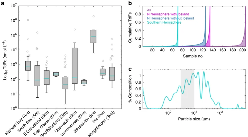
Fig. 1Iceberg iron and particle content.aIceberg iron (total dissolvable Fe) content per catchment. Boxes show median, 25thand 75thpercentiles; whiskers
show 10thand 90thpercentiles; dots mark all outliers. Regions: Antarctica (Ant), Greenland (Grn), Iceland (Ice), Patagonia (Pat), Svalbard (Sval). Data only
[image:2.595.87.510.443.678.2](p< 0.003) relative to all other catchments. Differences in Fe content between all other catchments and regions were insignif-icant (p> 0.9, see Supplementary Note 2 and Supplementary Tables 1 and 2). When samples from Jökulsárlón are excluded, the median TdFe concentration for catchments ranges from 44–790 nM. This is consistent with the limited iceberg Fe mea-surements from previous studies (20–290 nM, n=5)3,29–31. Furthermore, the global mean 9.3 µM Fe (excluding Jökulsárlón) is comparable to previous estimates of mean iceberg labile Fe content scaled-up from ascorbic acid leaches of glacial sediments and estimated iceberg sediment load (6.8 µM, using an estimate of 0.5 g sediment L−1 in icebergs)4,6. The exceptionally high Fe (mean and median of 310 µM and 93 µM respectively) for Jökulsárlón is likely due to the volcanic ash that is visibly present within this ice. Whilst volcanic enrichment of glacier-ice is not unique to Iceland32, it is uncommon and thus these data are excluded from the global mean forflux calculations.
With ice discharge from Greenland and Antarctica of ~500 and 1100 km3yr−133,34, respectively, the mean (9.3 µM) global iceberg Fe concentration corresponds to iceberg fluxes of 4.3 and 10 Gmol Fe yr−1. However, whilst our mean Fe concentration suggests fluxes at the upper end of previous estimates, which produce large global fluxes relative to other Fe supply mechan-isms16, the high variability in Fe content may have consequences for both Fe transfer to the open ocean and fertilization because 4% of ice sampled contains 91% of the Fe (Fig.1b). This highly heterogeneous Fe distribution is evident throughout the global dataset, in both the Arctic and Antarctic data irrespective of whether the Icelandic (Jökulsárlón) samples are excluded or not (Fig.1b). Such a distribution raises questions about the fate of Fe-rich iceberg layers in the marine environment, as these account for the vast majority of the total iceberg-to-ocean Feflux.
How efficient is iceberg-Fe-delivery. Regional Fe budgets and models for the marine environment generally assume that all supplied Fe is equal, i.e. that one unit of Fe delivered from atmospheric deposition has the same fertilizing effect as one unit of Fe delivered from icebergs if both sources overlap in time and space. However, several aspects of glacier-derived Fe sources are poorly constrained and these knowledge gaps may explain why modeled iceberg fertilization scenarios diverge between different model simulations; even when similar, and apparently con-servative, mean ice Fe concentrations are used (e.g. refs. 17,18). The general agreement between our estimate of iceberg TdFe concentration (mean of 9.3 µM) and a methodologically inde-pendent estimate of labile Fe within icebergs (mean of 6.8 µM, assuming a sediment load of 0.5 g L−1)4, suggests that the mean Fe content of icebergs is surprisingly well constrained on a global scale.
In addition to the approximate order of magnitude uncertainty in iceberg Fe concentration shown in prior work, sparse information is available on how Fe is distributed across the dissolved-particulate size continuum within ice25, how the speciation of Fe from ice melt affects its biological utilization in the ocean35, how changes in Fe distribution and concentration in ice after calving affect Fe delivery36 and what depth distribution this Fe is delivered over from melting icebergs18. Even with improved constraints on the total dissolvable Fe (TdFe) content of ice (Fig. 1a), several unknowns remain in how efficiently this Fe fuels marine primary production and ultimately C export to the deep ocean.
With respect to the lithogenic particle size within ice, several insights can be gained from our dataset. Earlier estimates of iceberg Fe content were deduced using estimated sediment loads within ice with a mean value of ~0.5 g L−1, producing iceberg labile Fe contents that are similar to the mean TdFe
concentrations presented herein4 and to a radium-derived sediment load estimate of 0.6–1.2 g L−1 for icebergs in the Weddell Sea6. However, the size and distribution of this material within ice is a further cause of substantial uncertainty. Whilst labile Fe content in glacially-derived sediment does not appear to vary substantially with particle size4,37, large lithogenic particles have shorter residence times in marine waters due to rapid sinking. A sediment size analysis (n=51, Svalbard iceberg samples38) suggests a mean particle size of 8.5 µm, which is comparable to the coarse size fraction (~3–10 µm, United States Environmental Protection Agency definition) of atmospheric dust (Fig.1c). In addition to particle size, the mineral speciation of Fe in particles can affect its solubility and bioaccessibility to marine biota39. In this respect, iceberg-derived sediment contains twice as much ferrihydrite, the most labile Fe mineral fraction, as atmospheric dust4,6,40, potentially making it a more effective fertilizer if delivered in a comparable way to the surface ocean. In summary, solid-state speciation and size analysis suggests that icebergs should be a relatively efficient Fe-fertilizer4.
A further poorly defined factor is the distribution of Fe within ice. Iceberg Fe concentrations are clearly highly variable (Fig.1b), with the range of measured concentrations being large compared to other freshwater-associated Fe supply mechanisms. For example, total Fe concentrations in rainwater range over two orders of magnitude from ~10 to 1000 nM41,42, and river water from ~0.1 to 100 µM43,44. The 6-order of magnitude range for icebergs (2 nM–2 mM) reflects the compositional difference between Fe-rich basal ice and non-basal ice, which contains only low concentrations of Fe derived from atmospheric deposition23. Such a large range in Fe concentrations within individual icebergs due to this inherent contrast likely explains why regional, or catchment specific, differences in Fe concentrations are not evident in a global dataset of this size (Fig.1). This heterogeneous distribution underpins the difference between the global 9.3 µM mean and 170 nM median iceberg Fe content, and raises questions about how this affects the lateral and vertical distribution of Fe input into the ocean from iceberg melt. The fertilization potential of particle and Fe-rich iceberg layers may depend on where these layers are located, and at what depth the associated meltwater is released into the ocean.
Fe release from melting icebergs. In order to explore how the rate at which the Fe content of iceberg meltwater varies with time after calving, we incorporate Fe content into a model in which iceberg melt rates have been constrained using observational data45. Fe fluxes from iceberg melt may vary as a function of iceberg geometry, iceberg spatial distribution, time and environ-mental drivers (e.g., ocean temperature and salinity, wind speed, air temperature, shortwave radiationflux and sea-ice concentra-tion). As catchment-specific observations are required to compute iceberg melt rates, we use summertime data from Sermilik fjord (Southeast Greenland), the only catchment globally for which iceberg distribution, morphology, size and melt rates have been previously constrained45,46.
as either only affecting the portion of an iceberg near the waterline (as previously45, Fig.2a), or as affecting the entire iceberg face50 (Fig.2b), with the most realistic formulation presently unclear. If the later approach is used in Sermilik, melt increases substantially over timescales within the typical fjord residence time, with many icebergs reaching a point of instability where inversion or disintegration becomes inevitable (open dots in Fig.2b).
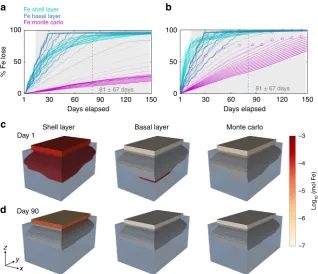
In both cases, disproportionately high loss of Fe from icebergs occurs within a few days to weeks of calving (Fig. 2a, b). The Monte Carlo distribution, which represents how iceberg Fefluxes have been estimated and typically modeled to date, results in a 10–70% decline in iceberg Fe content over the mean iceberg transit time of Sermilik Fjord (Fig.2a, b, magenta lines) depending on iceberg size and how wave-melt driven iceberg erosion is parameterized. This is coincident with a 10–70% decline in iceberg volume. However, the shell and basal scenarios result in 60–99% loss of Fe over the same time period (Fig.2a, turquoise and blue lines) for the same ice volume loss. This is consistent with the spatial distribution of ice-rafted debris in Sermilik fjord sediment cores51, which decreases away from Helheim glacier. Fe lost in this near-shore environment is unlikely to enhance primary produc-tion, as coastal waters are already fertilized by Fe from runoff and sedimentary sources52.
Our model simulations demonstrate that the post-calving age of an iceberg has a strong influence on its remaining Fe content, with the rate of Fe loss highly dependent upon the initial Fe distribution (Fig.2). Further complexities certainly arise between catchments due to differences in ocean temperature, iceberg size distribution, coastal ocean dynamics and uncertainty in the
thickness of basal ice. Basal ice thickness is poorly constrained and therefore here we defined the high Fe layers as occupying 9% of ice volume att=0 based on the observed distribution of TdFe (Fig.1b)6,36. Reducing this would amplify the difference between basal/shell and Monte Carlo scenarios (Fig. 2). Given the relatively fast loss of Fe that occurs from basal and shell layers in Sermilik within a few days of calving (Fig.2a, b), we may still have underestimated the extent of Fe loss in these scenarios because our iceberg samples (Fig.1) represent ice which calved a few days prior, rather than the marine-terminating glacier ice endmember.
An alternative iceberg melt model aiming to constrain sediment deposition, which should therefore also apply to particulate Fe within ice6,23,38, similarly estimated that 70–85% of iceberg-borne sediment was deposited within Kangerdlugssuaq fjord (E Greenland)36. Nevertheless, both of these model simulations represent Arctic marine-terminating glaciers in fjord systems where icebergs have a moderately long residence time (81 ± 67 days for Sermilik46) and are exposed to relatively warm ocean waters (1–4 °C in Sermilik summertime surface waters45) before entering the Atlantic Ocean. We therefore consider that, in a global context, our simulated basal and shell scenarios for these conditions (Fig. 2) represent approximate lower bounds for the fraction of Fe entering the Atlantic Ocean from icebergs. Reduced uncertainty concerning the spatial distribution of ice and Fe loss in other catchments will only be possible once further observational data becomes available and Fe/sediment distribution scenarios are better defined. This is especially the case with respect to regional differences in iceberg dimensions and sediment distribution.
150 120 81 ± 67 days 81 ± 67 days
90 Days elapsed
–3
–4
–5
Log
10
(mol F
e
)
–6
–7
60 30 100
a b
c
d
50
0 100
% F
e
loss
Fe shell layer
Fe basal layer Fe monte carlo
50
0
1 150 120 90 Days elapsed
Shell layer Day 1
Day 90
z
y x
Basal layer Monte carlo 60
30 1
Fig. 2Cumulative Fe release from different icebergs. Fe is initially distributed either randomly in a Monte Carlo simulation, concentrated in a layer of basal ice, or concentrated in a shell around the iceberg periphery. Icebergs of varying morphology, based on observed distributions, are released into Sermilik fjord at t=0 days.aMean net Fe loss from all icebergs within each Fe scenario. Days elapsed represents the model run length with mean iceberg residence time (dashed vertical line) ± standard deviation (shaded gray area) within Sermilik fjord shown for reference46. Thicker lines correspond to
increasing iceberg length (from 50 to 1000 m). Wave melt is parameterized as previously45.bThe same scenarios, but with an alternative
parameterization for wave-melt driven iceberg erosion50. Open dots represent icebergs reaching a point of instability where rolling or disintegration
[image:4.595.138.457.49.323.2]Whilst we observe no significant differences in TdFe between catchments herein (Fig.1), the dataset is biased towards sampling of smaller ice fragments (<20 m length above the waterline) which were originally calved from marine-terminating glaciers rather than large ice shelves. While Fe concentrations within terrestrial ice cores and marine ice (formed at the base of some ice shelves) overlap with the TdFe range we report for icebergs herein53, critical differences in the distribution of TdFe within recently-calved icebergs may still occur between catchments. This may especially be the case for ice calved from large ice shelves compared to ice calved from inshore marine-terminating glaciers, as the pathways for sediment incorporation into ice (and thus sediment loss from ice) differ between these scenarios and are not well characterized53,54. Critical unresolved questions are: how thick are Fe-rich layers, where are they located within different icebergs, how fast are these layers eroded in the marine environment, and how does this vary regionally?
The depth dependence of melt. Alongside the distribution of Fe within aging icebergs, the depth distribution of iceberg melt injection is a further interconnected issue widely acknowledged to affect the efficiency of iceberg-Fe delivery to the ocean mixed layer22,26,45, yet poorly constrained in the global ocean. In Ser-milik, 68–78% of summertime iceberg melt is injected into water beneath the shallow (10–20 m) surface layer, with this fraction predicted to remain entirely below the surface throughout sum-mer45. However, this finding provides limited insight into the behavior of meltwater around large icebergs in the open ocean, where the mixed layer is deeper and melt rates are generally lower (e.g. Supplementary Note 1 and Supplementary Fig. 1).
Whilst plume theory is reasonably well developed to approx-imate the behavior of subglacial discharge in 2 or 3 dimensional water columns55–57, subsurface iceberg melt behavior is less well constrained. Submarine melt rates are imperfectly matched by theoretical calculations58, and both the non-static nature of icebergs and the dilute nature of iceberg-associated plumes makes them challenging to define. It is a widespread hypothesis that iceberg melt upwells water to the ocean surface, with plumes of melt-modified water then spreading laterally away from icebergs enriched in the micronutrient Fe7. Evidence for such upwelling has indeed been observed around icebergs in some cases, yet is also notably intermittent and highly-spatially variable22,24,59. The behavior of meltwater in the water column depends strongly on ambient ocean conditions59, particularly the relative iceberg-ocean velocity. High relative velocities may lead to a detachment of meltwater plumes from the iceberg face and a broader distribution of meltwater through the water column21.
Idealized buoyancy plume calculations can be conducted for an iceberg in any region where water column properties are defined, and indicate that the fraction of ice melt upwelled to the surface and the fraction of ice melt injected below the mixed layer vary45 (e.g. see Supplementary Fig. 1). Yet the practical application of this to icebergs in a dynamic ocean is presently limited due to uncertainties with respect to the parametrization of melt rates58, as noted for wave induced melt (Fig.2a, b), a paucity of close-to-iceberg data to verify such calculations and the fundamentally weak and intermittent nature of iceberg melt plumes in the ocean. The mixing dynamics between melt and ocean waters remains a key uncertainty in how Fe from ice enters the ocean, and the extent to which it is subsequently made available to micro-organisms within the mixed layer21,22. We note that, given the heterogeneous distribution of Fe within icebergs, and the variable fraction of subsurface ice melt that may be brought to the surface or into the mixed layer (Supplementary Fig. 1), it is important in
future work to constrain how these two features interact — especially with respect to submerged basal layers.
Implications for Fe supply to phytoplankton. Defining iceberg Fe concentration shortly after calving is a bottom-up approach to defining the Feflux from icebergs by investigating total iceberg Fe concentrations. Equally important insight into the utilization efficiency of iceberg-derived Fe can be gained from a top-down approach, such as by using satellite-derived chlorophyll data in iceberg affected regions5,8,9. Given that iceberg Fe concentrations (Fig.1) suggest iceberg Fefluxes into the ocean are at the upper end, or greater than earlier estimates, it is perhaps useful to revisit prior attempts to define the efficiency with which iceberg-derived Fe is utilized on a regional scale. Regional Fe utilization was previously estimated as 7–14 µmol m−2yr−1 in areas of the Southern Ocean around the Antarctic Peninsula predicted to have a total iceberg derived supply of 72–726 µmol m−2yr−1 5. In contrast, regions with significant modeled atmospheric dust deposition (11–38 µmol m−2yr−1), such as down-wind of Pata-gonia, South Africa, and Australia60,61, had an Fe utilization that matched the modeled atmosphericflux5. The apparent difference between Fe supply and utilization for icebergs was attributed to potential temporal mismatches between supply and demand. However the spatial overlap of multiple Fe sources downstream of the Antarctic Peninsula makes it challenging to determine from satellite-derived data alone how efficient icebergs are as a source of Fe to surrounding waters5,17,18. Furthermore, satellite-derived chlorophyll data is less reliable at high latitudes62. Nevertheless, updating the total Feflux to values at the upper end of the previously used range would amplify the apparent mis-match. However, this also raises a critical question concerning the heterogeneous nature of Fe in icebergs across any region (Fig.1b): is it approximately correct to assume that this Fe will be spread evenly across the ocean, or approximately valid to esti-mate the potential fertilizing effect of icebergs from the total Fe flux or mean iceberg TdFe concentration? Furthermore, it is unclear on how broad a scale Fe-fertilization from icebergs operates. An influence of iceberg passage is generally observed on phytoplankton and nutrient distributions in iceberg tracks during the growth season9,12,23, but the regional effects of ice-bergs are more challenging to deduce from satellite derived data alone and are still subject to considerable uncertainties between models17,18. Identifying and tracking areas of iceberg Fe-enrichment is inherently difficult and thus any calculations to establish utilization rates are more challenging than for some other Fe sources5.
downstream of the intense inorganic Fe outflows of large glaciers66,67. Such a constraint challenges the assumption that mean, or total, iceberg Fe content can be used to predict broad-scale biological effects because the capping effect of ligand availability could strongly moderate the transfer of iceberg-derived Fe from Fe-rich ice.
We illustrate this by considering a mixing scenario between ice melt and Fe-deficient waters with an excess ligand concentration. Taking the freshwater excess calculated in melt enriched layers in iceberg-affected regions of the Weddell Sea suggests a melt water enrichment of ~0.1%22. Assuming, unrealistically, this was uniformly distributed through the surface mixed layer with total measured Fe ligand concentrations in this region ranging 1.2–2.4 nM65, the maximum quantity of Fe that could be transferred into the dissolved phase in the surface mixed layer would be a freshwater endmember of ~1.2–2.4 µM. This assumes the residence time of ice-derived particles in the mixed layer is short, exchange between particulate and dissolved Fe phases is rapid and that iceberg melt is occurring in Fe-deficient waters. The maximum enrichment possible would be lower in regions where primary production was not Fe-limited, or where multiple Fe-sources overlapped65, and slightly higher in surface waters due to photochemical processes creating soluble dissolved Fe(II)65. For icebergs with a TdFe concentration close to the median (170 nM), a large fraction of the labile Fe present could therefore potentially be transferred to the dissolved phase. However, this declines to only 13–26% for icebergs with TdFe close to the mean (9.3 µM). Such a calculation is over-simplistic in many respects as it neglects to consider the different depths of intrusions and mechanisms of melt occurring in the water column22. Furthermore, it is unclear on what spatiotemporal scales iceberg-derived particulate Fe is removed from the water column and how quickly the labile particulate and dissolved Fe phases achieve equilibration. Never-theless, for ice with high TdFe content, a high fraction of iceberg TdFe could plausibly be maintained in the mixed layer only under
very dilute meltwater addition scenarios. Therefore, the use of a mean iceberg Fe content to represent highly variable iceberg Fe input into the ocean from a point source delivered at the surface is questionable18.
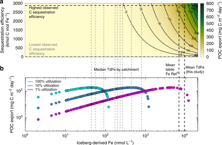
Uncertainties in C export from iceberg fertilization. Given the range of uncertainties, estimates of the extent to which iceberg-derived Fe enhances primary production7–9 and C export vary significantly7,17,68. This is especially the case in the Fe-limited Southern Ocean, where iceberg Fe fertilization is expected to have the greatest stimulatory effect69, but the relationship between Fe input and C export is complex70. The simplest method for esti-mating how any Fe input into the ocean affects C export, the quantity of POC sinking beneath 100 m depth, is by using Fe-to-C sequestration efficiencies71,72. Fe-to-C sequestration efficiencies have been estimated for several naturally Fe-fertilized, high-latitude regions (including the Crozet Islands, Kerguelen Plateau and Irminger Basin71–73). Yet Fe-to-C sequestration efficiencies vary widely from 17 to 2900 Kmol C mol−1 Fe and are thus challenging to apply at broader scales71,73. Even if they are applied to a specific regional ice melt Fe-enrichment scenario, for example the simplistic ~0.1% melt water enrichment scenario outlined above, a very broad range of POC export is plausible considering the range of iceberg Fe content (Fig.3a). The mean iceberg TdFe concentration, coupled with an intermediate or high C sequestration efficiency would produce a high C export. Yet a median iceberg TdFe concentration would correspond to C export an order of magnitude lower irrespective of the C sequestration efficiency (Fig. 3a). Additionally, none of these calculated sequestration efficiencies concern regions where ice-bergs are thought to dominate Fe supply.
An alternative method to convert iceberg Fe input into plausible POCfluxes is to use an estimate of Fe:C cellular ratios to calculate the primary production potentially supported by an
3000 a
b
800 700 600 500 400 300
POC e
xpor
t (mg C m
–2
da
y
–1)
POC e
xpor
t (mg C m
–2
da
y
–1
)
200
100
Median TdFe by catchment Mean TdFe
(this study) Mean
labile
Fe Ref4
0 2500
Highest observed C sequestration efficiency
Lowest observed C sequestration efficiency
100% utilization 10% utilization 1% utilization
2000
1500
Sequestr
ation efficiency
(kmol C mol F
e
–1)
1000
500
102
100
100 101 102
Iceberg-derived Fe (nmol L–1)
103 104
0
Fig. 3Estimating C exportfluxes. Following fertilization of Fe-limited waters for a regional 0.1% meltwater enrichment, C export is estimated using two different methods.aFe-to-C sequestration efficiencies estimate the organic Cflux to > 100 m depth following Fe fertilization. Vertical lines correspond to the median TdFe of ice each catchment (gray dashed lines), mean labile Fe derived from estimates of iceberg sediment content and mean TdFe for this dataset (black dashed lines).bPOC export is estimated for 1, 10 and 100% Fe utilization (the percentage of Fe supply up-taken by biota) scenarios. This Fe supply is combined with Fe:C cellular ratios and the observed trend between surface primary production and C export efficiency in the Southern Ocean74.
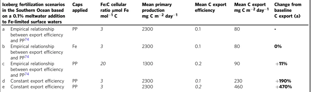
[image:6.595.119.476.437.670.2]Feflux and then to use the observational trend between primary production and C export to deduce the resulting POC flux (Fig.3b). The fraction of C formed by primary production which is ultimately exported to depth is however also subject to pronounced spatiotemporal variation. C export efficiency, ran-ging from 0–1, is defined as the fraction of organic C formed by primary production that is exported below 100 m depth, and observational evidence suggest that this efficiency generally declines with increasing primary production74. Calculating the potential primary production supported by an Fe input from Fe:C cellular ratios of 3–20 µmol Fe mol−1 C, again for a specific ~0.1% melt water enrichment scenario for simplicity, with a mixed layer depth of 100 m, and a constant iceberg fertilization effect lasting a month7,22, the uncertainty in C export efficiency amplifies the uncertainty in iceberg-Fe fluxes into the surface mixed layer (Table1).
In scaling Fe input to primary production using Fe:C cellular ratios, the effect of applying a cap to primary production (e.g. 3000 mg C m−2day−1) or to the maximum stable concentration of Fe in the water column (e.g. 2 nM), approximating upper limits to observed values23,74, is the same (Table 1a, b). A more significant query is how C export is scaled to primary production. Southern Ocean observational studies, using both sediment traps and thorium-234 based estimates of POC export, suggest a pronounced decline in C export efficiency with increasing primary production in both spring and summer74. Yet such a relationship between primary production and C export efficiency is not reproduced in most biogeochemical models (e.g. ref.18) or accounted for in some iceberg POC export calculations (e.g. ref. 7), meaning that differences in estimates of iceberg-Fe-fertilization can arise from how Fe is scaled to C export independently of how the iceberg Feflux is quantified.
Aside from the general question concerning how C export scales with primary production in the high-latitude oceans75, a more specific question is whether iceberg fertilized regions will deviate from the background trend in any region. Do icebergs have a unique primary production-C export relationship due to mixing effects, biological community shifts, ballasting effects from lithogenic particles or other features unique to icebergs12,15,68? While there is limitedfield evidence that icebergs locally enhance C export15,68, there is insufficient evidence to evaluate if the presence of icebergs results in significant changes to regional C export efficiency. It is presently unclear on what spatiotemporal scales iceberg-induced changes to C export operate because
enhanced primary production can lag behind iceberg passage by days to weeks and thus fertilized regions can be detached from the immediate vicinity of icebergs7,9,12. Furthermore, in addition to the short-term fertilization following Fe release into the surface mixed layer considered in both ship-based and satellite-based approaches9,12, increasing concentrations of Fe at depth could have a weaker but more widespread fertilizing effect on longer inter-annual timescales18.
In summary, the utilization of iceberg-derived Fe in the marine environment is challenging to determine and a broad range of C export scenarios are plausible for any specific Fe addition and ice melt mixing scenario (e.g. Fig. 3). We note that if C export in the high-latitude oceans does not always scale proportionately with summertime primary production (which is what observa-tional studies suggest70,74), Fe may more efficiently fuel C export when a dilute Fe addition induces low primary production with high C export efficiency, than when a concentrated Fe addition induces high primary production but with low C export efficiency (Fig.3b).
With increasingfluxes of solid ice discharge into the ocean, the importance of icebergs as a source of Fe to the ocean is widely expected to increase11,76,77. Using global observations, we demonstrate that total Fe fluxes from icebergs into the ocean are already in excess of 14 Gmol Fe yr−1. However, iceberg Fe concentrations are extremely variable (Fig. 1b). This directly affects the potential fraction of Fe transferred into the open ocean (Fig.2), the subsequent distribution of Fe at the point of injection into the ocean and therefore the efficiency with which this Fe can stimulate primary production and C export. In order to reduce uncertainty concerning iceberg ocean fertilization, future para-meterizations of this phenomenon in global ocean biogeochem-ical models must account for heterogeneity in iceberg morphology and Fe content. This will require integration of iceberg-Fe distributions into iceberg melt models. Due to the sensitivity of iceberg Fe delivery to iceberg morphology and internal Fe distribution (Fig. 2), climate-driven changes in the spatiotemporal footprint of iceberg melt may influence marine productivity more than changes in total iceberg Feflux into the ocean —a feature which is yet to be considered in forecasts of ocean productivity under future climate scenarios.
Methods
Ice samples. Low-density polyethylene (LDPE) sample bottles were pre-cleaned in
[image:7.595.44.553.84.235.2]a three stage procedure (detergent, 1 M HNO3, 1 M HCl) and then stored double
Table 1 Conversion between Fe, primary production (C) and C export, for a specific scenario where a uniform mixed layer of 100 m is fertilized with a 0.1% meltwater enrichment for each iceberg in the global dataset
Iceberg fertilization scenarios in the Southern Ocean based on a 0.1% meltwater addition to Fe-limited surface waters
Caps applied
Fe:C cellular ratioµmol Fe mol−1C
Mean primary production mg C m−2day−1
Mean C export efficiency
Mean C export mg C m−2day−1
Change from baseline C export (a)
a Empirical relationship between export efficiency and PP74
PP 3 2300 0.1 80
-b Empirical relationship between export efficiency and PP74
Fe 3 2300 0.1 80 0%
c Empirical relationship between export efficiency and PP74
PP 20 1300 0.2 90 +11%
d Constant export efficiency PP 3 2300 0.1 230 +190%
e Constant export efficiency PP 3 2300 0.2 460 +470%
Caps are applied either to primary production (PP, max 3000 mg C m−2day−1) or Fe concentration (post-mixing max 2 nM). C export efficiency (the fraction of organic C exported beneath 100 m depth)
bagged until required in thefield. Iceberg samples were collected by hand using
metal-free tools. Sample collection was randomized at eachfieldsite location by
collecting ice samples at regular intervals along pre-defined transects using small
boats. Targeted icebergs had visible widths of 0.5–20 m above the waterline. In total 1–5 kg ice pieces were retained in LDPE bags and melted at room temperature. The
first 4 aliquots of meltwater were discarded. 125 mL of meltwater was retained
unfiltered in trace metal clean LDPE bottles. Trace metal samples were then
acidified to pH 1.9 by addition of 180 µL HCl (UPA, ROMIL) and allowed to stand
upright for >6 months prior to analysis via inductively-coupled, plasma mass
spectrometry (Element XR, ThermoFisher Scientific) after dilution with 1 M HNO3
(distilled in-house from SPA grade HNO3, Roth). Calibration was via standard
addition with a linear peak response from 1 to 1000 nM Fe (R2> 0.99). Analysis of
the reference material CASS-6 (n=12) yielded a Fe concentration of 26.6 ± 1.2 nM
(certified 27.9 ± 2.1 nM). 51 sediment samples collected from iceberg surfaces or
from embedded within icebergs (as per Ref.38) and stored frozen were defrosted at
room temperature and analyzed for particle size distributions within the size range 0.1–1000 µm using a Laser Analysette.
In addition to previously unpublished data from 152 new samples collected and analyzed herein, existing comparable data was compiled from prior work in
Greenland29,63, Svalbard38and Antarctica3,23,30,31,78and is included in the global
average iceberg composition. Previously published data from Godthåbsfjord (n=
9)63, Kongsfjorden (n=28)38, South Bay (n=7)78and Maxwell Bay (n=7)78is
included alongside new data in these catchments (e.g. Fig.1a).
Iceberg melt model experiments. To quantify variability in iceberg Fe content and distribution under realistic melting conditions, we used an iceberg melt
model45constrained by ice, ocean, and meteorological conditions in Sermilik Fjord.
Time- and depth-dependent iceberg geometry (i.e., width, length, keel depth, and
freeboard height) was used to produce 3–D representations of iceberg volume and
Fe concentration at daily time steps. The horizontal and vertical grid resolution was
1 m, with fractional grid cells used for ice volumes < 1 m3. Iceberg lengths from 50
to 1000 m (at 50 m intervals) were simulated; we then scaled the ice volume and Fe concentration by the observed iceberg distribution in Sermilik fjord to compute net
ice volume and Fe loss, respectively (Fig.2).
The dominant decay term in iceberg melt is often wave erosion of the iceberg’s
vertical faces. Previously using this iceberg melt model45the wave erosion term was
defined as affecting only an area equal to the wave amplitude above and below the
waterline. Over short time periods (<8 days), there is minimal difference between this formulation and one where wave erosion is applied to the entire iceberg
vertical face (the difference being included within the uncertainty in ref.45).
However, for longer time periods which are comparable to the residence time within Sermilik fjord (mean of 81 days), the difference between these two wave-melt formulations becomes larger. Both approaches are therefore considered
(Fig.2a, b). Furthermore, over this longer time period some icebergs, especially
towards the smaller end of the modeled range (50–1000 m length) become unstable
(defined as length/width/depths which would be likely to capsize and/or initiate
disintegration into multiple smaller icebergs). As modeling such instability or
fragmentation is challenging and unsupported byfield observations, icebergs
reaching a point of instability are therefore removed from the model run (as
indicated by open dots on Fig.2a, b).
We tested 3 idealized iceberg Fe distribution scenarios: a shell distribution, a layer distribution, and a Monte Carlo distribution. For the shell and basal-layer cases, high and low Fe ice was set to 100 µM and 170 nM, respectively; grid cells with high Fe constituted 9% of the total iceberg volume representing the 9% of
samples with TdFe > TdFemean. For the shell case, the albedo for the iceberg top
and above-freeboard sides was reduced from 0.7 to 0.3 when high Fe ice was
present (representing the influence of sediment-rich ice)79. The Monte Carlo case
assigned Fe concentrations, randomly sampled from the observational dataset, to random grid cells until the total Fe content was equal to the shell case; all cells not assigned by the Monte Carlo method were set to low Fe ice. Iceberg simulations
started on May 1stand were time stepped for 180 days. Basal layer thickness is
poorly defined in the literature with general estimates of <3–10 m6,36. Here we used
a fractional composition of 9% high Fe for basal/shell scenarios based on the TdFe data distribution. For substantially thinner basal layers, the difference between
Basal/Shell and Monte Carlo scenarios in Fig.1would be amplified.
Primary production and C export calculations. Fe supply to primary producers
was calculated as 2× the extrapolatedflux from iceberg TdFe concentrations i.e.
using a 1/fe ratio of 2 for high Fe waters5,80. Except where stated otherwise, a
constant cellular Fe:C ratio wasfixed as 3 µmol Fe mol−1C81. The relationship
between primary production and C export was determined using data from Ref.74
and thefit C export efficiency=−0.3484 × Log(PP)+1.2239 with a cap applied at
zero export to prevent negative values in C export. Except where stated otherwise,
C export is defined at 100 m, and the mixed layer is defined as 0–100 m.
Data availability
All new data is available in the main text or the Supplementary Materials. Source data for iceberg TdFe concentrations underlying Figs.1–3are provided as a Source Datafile (Supplementary Material).
Code availability
The modified code for Fe release from melting icebergs (originally from ref.45) is
available fromhttps://github.com/dcarrollsci/iceberg_Fe_model.
Received: 13 March 2019; Accepted: 29 October 2019;
References
1. Hart, T. J. Discovery Reports.Discov. Rep.VIII, 1–268 (1934).
2. Raiswell, R., Benning, L. G., Tranter, M. & Tulaczyk, S. Bioavailable iron in the
Southern Ocean: the significance of the iceberg conveyor belt.Geochem. Trans.
9, 7 (2008).
3. Loscher, B. M., DeBaar, H. J. W., DeJong, J. T. M., Veth, C. & Dehairs, F. The
distribution of Fe in the Antarctic Circumpolar.Curr. Deep. Res. Part
Ii-Topical Stud. Oceanogr.44, 143–187 (1997).
4. Raiswell, R. et al. Potentially bioavailable iron delivery by iceberg-hosted
sediments and atmospheric dust to the polar oceans.Biogeosciences13,
3887–3900 (2016).
5. Boyd, P. W., Arrigo, K. R., Strzepek, R. & Van Dijken, G. L. Mapping
phytoplankton iron utilization: Insights into Southern Ocean supply
mechanisms.J. Geophys. Res. Ocean117, C06009 (2012).
6. Shaw, T. J. et al. Input, composition, and potential impact of terrigenous
material from free-drifting icebergs in the Weddell Sea.Deep. Res. Part
Ii-Topical Stud. Oceanogr.58, 1376–1383 (2011).
7. Duprat, L. P. A. M., Bigg, G. R. & Wilton, D. J. Enhanced Southern Ocean
marine productivity due to fertilization by giant icebergs.Nat. Geosci.9,
219–221 (2016).
8. Wu, S.-Y. & Hou, S. Impact of icebergs on net primary productivity in the
Southern Ocean.Cryosphere11, 707–722 (2017).
9. Schwarz, J. N. & Schodlok, M. P. Impact of drifting icebergs on surface
phytoplankton biomass in the Southern Ocean: Ocean colour remote sensing
and in situ iceberg tracking.Deep. Res. Part I Oceanogr. Res. Pap.56,
1727–1741 (2009).
10. Smith, K. L. Jr et al. Free-drifting icebergs: Hot spots of chemical and
biological enrichment in the Weddell Sea.Science317, 478–482 (2007).
11. Smith, K. L., Sherman, A. D., Shaw, T. J. & Sprintall, J. Icebergs as
unique lagrangian ecosystems in polar seas.Ann. Rev. Mar. Sci.5, 269–287
(2013).
12. Vernet, M., Sines, K., Chakos, D., Cefarelli, A. O. & Ekern, L. Impacts on phytoplankton dynamics by free-drifting icebergs in the NW Weddell Sea. Deep Sea Res. Part II Top. Stud. Oceanogr.58, 1422–1435 (2011). 13. Paolo, F. S., Fricker, H. A. & Padman, L. Volume loss from Antarctic ice
shelves is accelerating.Science348, 327 LP–327331 (2015).
14. Bamber, J., van den Broeke, M., Ettema, J., Lenaerts, J. & Rignot, E. Recent
large increases in freshwaterfluxes from Greenland into the North Atlantic.
Geophys. Res. Lett.39, L19501–L19501 (2012).
15. Smith, K. L. et al. Carbon export associated with free-drifting icebergs in the
Southern Ocean.Deep. Res. Part II Top. Stud. Oceanogr.58, 1485–1496 (2011).
16. Tagliabue, A. et al. How well do global ocean biogeochemistry models
simulate dissolved iron distributions?Glob. Biogeochem. Cycles30, 149–174
(2016).
17. Laufkötter, C., Stern, A. A., John, J. G., Stock, C. A. & Dunne, J. P. Glacial iron
sources stimulate the southern ocean carbon cycle.Geophys. Res. Lett.45,
377–13,385 (2018).
18. Person, R. et al. Sensitivity of ocean biogeochemistry to the iron supply from
the Antarctic ice sheet explored with a biogeochemical model.Biogeosciences
16, 3583–3603 (2019).
19. Wadley, M. R., Jickells, T. D. & Heywood, K. J. The role of iron sources and
transport for Southern Ocean productivity.Deep. Res. Part I-Oceanographic
Res. Pap.87, 82–94 (2014).
20. Death, R. et al. Antarctic ice sheet fertilises the Southern Ocean.Biogeosciences
11, 2635–2643 (2014).
21. FitzMaurice, A. C., Cenedese, C. & Straneo, F. Nonlinear response of
iceberg side melting to ocean currents.Geophys. Res. Lett.44, 5637–5644
(2017).
22. Stephenson, G. R. et al. Subsurface melting of a free-floating Antarctic iceberg.
Deep Sea Res. Part II Top. Stud. Oceanogr.58, 1336–1345 (2011). 23. Lin, H., Rauschenberg, S., Hexel, C. R., Shaw, T. J. & Twining, B. S.
Free-drifting icebergs as sources of iron to the Weddell Sea.Deep. Res. Part
II-Topical Stud. Oceanogr.58, 1392–1406 (2011).
24. Helly, J. J., Kaufmann, R. S., Stephenson, G. R. Jr & Vernet, M. Cooling, dilution and mixing of ocean water by free-drifting icebergs in the Weddell Sea.Deep. Res. Part II-Topical Stud. Oceanogr.58, 1346–1363 (2011). 25. Raiswell, R. et al. Iron in glacial systems: speciation, reactivity, freezing
26. de Jong, J. et al. Natural iron fertilization of the Atlantic sector of the Southern
Ocean by continental shelf sources of the Antarctic Peninsula.J. Geophys. Res.
117, G01029 (2012).
27. Klunder, M. B., Laan, P., Middag, R., De Baar, H. J. W. & Van Ooijen, J. C.
Dissolved iron in the Southern Ocean (Atlantic sector).Deep. Res. Part II58,
2678–2694 (2011).
28. Edwards, R. & Sedwick, P. Iron in East Antarctic snow: Implications for atmospheric iron deposition and algal production in Antarctic waters. Geophys. Res. Lett.28, 3907–3910 (2001).
29. Campbell, J. A. & Yeats, P. A. The distribution of manganese, iron, nickel,
copper and cadmium in the waters of Baffin Bay and the Canadian Arctic
Archipelago.Oceanol. Acta5, 161–168 (1982).
30. Martin, J. H., Gordon, R. M. & Fitzwater, S. E. Iron in Antarctic waters. Nature345, 156–158 (1990).
31. De Baar, H. J. W. et al. Importance of iron for plankton blooms and carbon
dioxide drawdown in the Southern Ocean.Nature373, 412–415 (1995).
32. van der Merwe, P. et al. High lability fe particles sourced from glacial erosion can meet previously unaccounted biological demand: Heard Island, Southern
Ocean.Front. Mar. Sci.6, 332 (2019).
33. Bamber, J. L. et al. Land Ice Freshwater Budget of the Arctic and North
Atlantic Oceans: 1. Data, Methods, and Results.J. Geophys. Res. Ocean.123,
1827–1837 (2018).
34. Rignot, E., Jacobs, S., Mouginot, J. & Scheuchl, B. Ice-shelf melting around
Antarctica.Science341, 266 LP–266270 (2013).
35. Kim, K., Choi, W., Hoffmann, M. R., Yoon, H.-I. & Park, B.-K. Photoreductive dissolution of iron oxides trapped in ice and its environmental implications. Environ. Sci. Technol.44, 4142–4148 (2010).
36. Mugford, R. I. & Dowdeswell, J. A. Modeling iceberg-rafted sedimentation in
high-latitude fjord environments.J. Geophys. Res. Earth Surf.115, F03024
(2010).
37. Hopwood, M. J., Statham, P. J., Tranter, M. & Wadham, J. L. Glacialflours as a
potential source of Fe(II) and Fe(III) to polar waters.Biogeochemistry118,
443–452 (2014).
38. Hopwood, M. J., Cantoni, C., Clarke, J. S., Cozzi, S. & Achterberg, E. P. The
heterogeneous nature of Fe delivery from melting icebergs.Geochemical
Perspect. Lett.3, 200–209 (2017).
39. Schroth, A. W., Crusius, J., Sholkovitz, E. R. & Bostick, B. C. Iron solubility
driven by speciation in dust sources to the ocean.Nat. Geosci.2, 337–340
(2009).
40. Raiswell, R. Iceberg-hosted nanoparticulate Fe in the Southern Ocean:
Mineralogy, origin, dissolution kinetics and source of bioavailable Fe.Deep.
Res. Part II-Topical Stud. Oceanogr.58, 1364–1375 (2011).
41. Kieber, R. J., Willey, J. D. & Avery, G. B. Temporal variability of rainwater
iron speciation at the Bermuda Atlantic time series station.J. Geophys. Res.
108, 3277 (2003).
42. Kieber, R. J., Williams, K., Willey, J. D., Skrabal, S. & Avery, G. B. Iron speciation in coastal rainwater: concentration and deposition to seawater. Mar. Chem.73, 83–95 (2001).
43. Neal, C. et al. Increasing iron concentrations in UK upland waters.Aquat.
Geochem.14, 263–288 (2008).
44. Neal, C. & Robson, A. J. A summary of river water quality data collected within the Land-Ocean Interaction Study: core data for eastern UK
rivers draining to the North Sea.Sci. Total Environ.251, 585–665
(2000).
45. Moon, T. et al. Subsurface iceberg melt key to Greenland fjord freshwater
budget.Nat. Geosci.11, 49–54 (2018).
46. Sutherland, D. A. et al. Quantifyingflow regimes in a Greenland glacial fjord
using iceberg drifters.Geophys. Res. Lett.41, 8411–8420 (2014).
47. Raiswell, R. & Canfield, D. E. The iron biogeochemical cycle past and present.
Geochem. Perspect.1, 1–220 (2012).
48. Bigg, G. R., Wadley, M. R., Stevens, D. P. & Johnson, J. A. Modelling the
dynamics and thermodynamics of icebergs.Cold Reg. Sci. Technol.26,
113–135 (1997).
49. Silva, T. A. M., Bigg, G. R. & Nicholls, K. W. Contribution of giant icebergs to
the Southern Ocean freshwaterflux.J. Geophys. Res. Ocean.111, C03004
(2006).
50. Wagner, T. J. W. et al. The“footloose”mechanism: Iceberg decay from
hydrostatic stresses.Geophys. Res. Lett.41, 5522–5529 (2014).
51. Andresen, C. S. et al. Rapid response of Helheim Glacier in Greenland to
climate variability over the past century.Nat. Geosci.5, 37–41 (2012).
52. Cape, M. R., Straneo, F., Beaird, N., Bundy, R. M. & Charette, M. A. Nutrient release to oceans from buoyancy-driven upwelling at Greenland tidewater
glaciers.Nat. Geosci.12, 34–39 (2019).
53. Herraiz-Borreguero, L., Lannuzel, D., van der Merwe, P., Treverrow, A. &
Pedro, J. B. Largeflux of iron from the Amery Ice Shelf marine ice to Prydz
Bay, East Antarctica.J. Geophys. Res. Ocean121, 6009–6020 (2016).
54. Winter, K. et al. Radar-Detected Englacial Debris in the West Antarctic Ice
Sheet.Geophys. Res. Lett.46, 10454–10462 (2019).
55. Morton, B. R., Taylor, G. & Turner, J. S. Turbulent gravitational convection
from maintained and instantaneous sources.Proc. R. Soc. A Math. Phys. Eng.
Sci.234, 1–23 (1956).
56. Jenkins, A. Convection-driven melting near the grounding lines of ice shelves
and tidewater glaciers.J. Phys. Oceanogr.41, 2279–2294 (2011).
57. Cowton, T., Slater, D., Sole, A., Goldberg, D. & Nienow, P. Modeling the impact of glacial runoff on fjord circulation and submarine melt rate using a
new subgrid-scale parameterization for glacial plumes.J. Geophys. Res. Ocean
120, 796–812 (2015).
58. Sutherland, D. A. et al. Direct observations of submarine melt and subsurface
geometry at a tidewater glacier.Science365, 369 LP–369374 (2019).
59. Yankovsky, A. E. & Yashayaev, I. Surface buoyant plumes from melting icebergs
in the Labrador Sea.Deep Sea Res. Part I Oceanogr. Res. Pap.91, 1–9 (2014).
60. Mahowald, N. M. et al. Atmospheric global dust cycle and iron inputs to the
ocean.Glob. Biogeochem. Cycles19, GB2006 (2005).
61. Wagener, T., Guieu, C., Losno, R., Bonnet, S. & Mahowald, N. Revisiting atmospheric dust export to the Southern Hemisphere ocean: biogeochemical
implications.Glob. Biogeochem. Cycles22, GB2006 (2008).
62. Johnson, R., Strutton, P. G., Wright, S. W., McMinn, A. & Meiners, K. M.
Three improved satellite chlorophyll algorithms for the Southern Ocean.J.
Geophys. Res. Ocean118, 3694–3703 (2013).
63. Hopwood, M. J. et al. Seasonal changes in Fe along a glaciated Greenlandic
fjord.Front. Earth Sci.4, (2016).
64. Johnson, K. S., Gordon, R. M. & Coale, K. H. What controls dissolved iron in
the world ocean?Mar. Chem.57, 137–161 (1997).
65. Lin, H. & Twining, B. S. Chemical speciation of iron in Antarctic waters
surrounding free-drifting icebergs.Mar. Chem.128, 81–91 (2012).
66. Lippiatt, S. M., Lohan, M. C. & Bruland, K. W. The distribution of reactive
iron in northern Gulf of Alaska coastal waters.Mar. Chem.121, 187–199
(2010).
67. Thuroczy, C.-E. et al. Key role of organic complexation of iron in sustaining phytoplankton blooms in the Pine Island and Amundsen Polynyas (Southern
Ocean).Deep. Res. Part II-Topical Stud. Oceanogr.71–76, 49–60 (2012).
68. Shaw, T. J. et al. 234th-based carbon export around free-drifting icebergs in
the Southern Ocean.Deep Sea Res. Part II Top. Stud. Oceanogr.58, 1384–1391
(2011).
69. Martin, J. H., Fitzwater, S. E. & Gordon, R. M. Iron deficiency limits
phytoplankton growth in Antarctic waters.Glob. Biogeochem. Cycles4, 5–12
(1990).
70. Le Moigne, F. A. C. et al. What causes the inverse relationship between
primary production and export efficiency in the Southern Ocean?Geophys.
Res. Lett.43, 800–4466 (2016).
71. Blain, S. et al. Effect of natural iron fertilization on carbon sequestration in the
Southern Ocean.Nature446, 1070–U1 (2007).
72. Pollard, R. T. et al. Southern Ocean deep-water carbon export enhanced by
natural iron fertilization.Nature457, 577–580 (2009).
73. Le Moigne, F. A. C. et al. Sequestration efficiency in the iron-limited North
Atlantic: Implications for iron supply mode to fertilized blooms.Geophys. Res.
Lett.41, 4619–4627 (2014).
74. Maiti, K., Charette, M. A., Buesseler, K. O. & Kahru, M. An inverse
relationship between production and export efficiency in the Southern Ocean.
Geophys. Res. Lett.40, 1557–1561 (2013).
75. Henson, S., Le Moigne, F. & Giering, S. Drivers of carbon export efficiency in
the global ocean.Glob. Biogeochem. Cycles33, 891–903 (2019).
76. Hutchins, D. A. & Boyd, P. W. Marine phytoplankton and the changing ocean
iron cycle.Nat. Clim. Chang6, 1072–1079 (2016).
77. Hoffmann, L., Breitbarth, E., Boyd, P. & Hunter, K. Influence of ocean
warming and acidification on trace metal biogeochemistry.Mar. Ecol. Prog.
Ser.470, 191–205 (2012).
78. Höfer, J. et al. The role of water column stability and wind mixing in the production/export dynamics of two bays in the Western Antarctic Peninsula. Prog. Oceanogr.174, 105–116 (2019).
79. Box, J. E. et al. Greenland ice sheet albedo feedback: thermodynamics and
atmospheric drivers.Cryosphere6, 821–839 (2012).
80. Boyd, P. W. & Ellwood, M. J. The biogeochemical cycle of iron in the ocean. Nat. Geosci.3, 675–682 (2010).
81. Fung, I. Y. et al. Iron supply and demand in the upper ocean.Glob.
Biogeochem. Cycles14, 281–295 (2000).
Acknowledgements
Code for the construction of Fig.2was adapted from that originally described in ref.45,
Author contributions
M.H., J.H., L.M., L.B., C.E., and H.G. conductedfieldwork and laboratory analysis; D.C. and D.S. undertook modeling work; D.C., F.M., and M.H. produced thefigures; M.H., D.C., F.M., and E.A. wrote the manuscript with all authors contributing to its revision.
Competing interests
The authors declare no competing interests.
Additional information
Supplementary informationis available for this paper at https://doi.org/10.1038/s41467-019-13231-0.
Correspondenceand requests for materials should be addressed to M.J.H.
Peer review informationNature Communicationsthanks Delphine Lannuzel, Thomas Rackow and other, anonymous, reviewers for their contributions to the peer review of this work. Peer review reports are available.
Reprints and permission informationis available athttp://www.nature.com/reprints
Publisher’s noteSpringer Nature remains neutral with regard to jurisdictional claims in published maps and institutional affiliations.
Open Access This article is licensed under a Creative Commons Attribution 4.0 International License, which permits use, sharing, adaptation, distribution and reproduction in any medium or format, as long as you give appropriate credit to the original author(s) and the source, provide a link to the Creative Commons license, and indicate if changes were made. The images or other third party material in this article are included in the article’s Creative Commons license, unless indicated otherwise in a credit line to the material. If material is not included in the article’s Creative Commons license and your intended use is not permitted by statutory regulation or exceeds the permitted use, you will need to obtain permission directly from the copyright holder. To view a copy of this license, visithttp://creativecommons.org/ licenses/by/4.0/.