Multiple prediction combination and confidence measures for marine object detection

A good generic object detection method will be effective on a variety of datasets. Three

image collections were used in testing the object detection algorithms in this thesis.

For the first (face detection) an existing cascade was used, so the only dataset required

was a collection of test images distinct from its training images. For the other sets

(fish and seahorse detection), cascades had to be trained before they were tested. This

required sufficient images to create separate training and testing sets.

It should be noted that both marine animal image sets contain multiple animals

per image, and therefore have more positive training samples than images. Also,

sec-tion 2.6.3 explains how the Haar Classifier Cascade training process searches through

its negative training images at different positions and scales to create negative training

samples for each stage. Each negative training image therefore offers a large number

of negative training samples.

4.1

Faces

Face detection is a common application for object detection algorithms, so cascades

already exist for detecting faces, and datasets already exist for testing them. A

com-monly used image set is the MIT/CMU frontal face testing dataset (Rowley et al.,

2003). These images were assembled to test a neural network-based face detector

(Rowley et al., 1998a), but are suitable for testing any frontal face detection

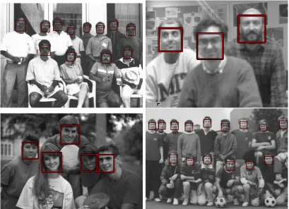
algo-rithm. All face detection testing in this thesis used MIT/CMU test sets A, B, and

C. These contain 130 images, including those in fig. 4.1, which between them contain

511 faces. Existing annotations giving the coordinates of both eyes and the left, centre

and right part of the mouth are provided. OpenCV requires rectangular annotations,

which were from the eye and mouth points as follows:

−−−−−→

eye_centre= −−−→eyelef t+−−−−→eyeright 2

−−−−−→

face_centre = −−−−−→eyecentre+

−−−−−−−→

mouthcentre

2

facewidth =

!

(eyelef tx −eyerightx)

2_{+ (eye}

lef ty−eyerighty)

2

face_height=!(eye_centrex −mouthcentrex)2+ (eyecentrey −mouthcentrey)2

face_size = 1.2_×(face_width+face_height)

face_x1 =face_{centrex −}facesize 2

face_x2 =face_centrex +facesize 2

face_y1 =face_centrey− facesize 2

facey2 =facecentrey+

face_size 2

Figure 4.1: Example face images

4.1.1

Cascade selection

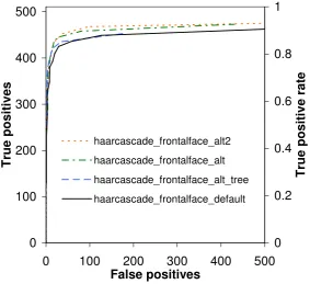
OpenCV is provided with four face detectors trained by Lienhart et al. (Lienhartet al.,

2003a): three cascades and a tree (Lienhartet al., 2003b). These were each run on the

MIT/CMU faces; the resulting ROC curves are plotted in fig. 4.3. The best overall

detector was haarcascade frontalface alt2, so it was used in the chapter 6 face detection

experiments. 0 100 200 300 400 500

0 100 200 300 400 500 False positives Tr ue pos it iv e s 0 0.2 0.4 0.6 0.8 1 Tr ue pos it iv e r a te haarcascade_frontalface_alt2 haarcascade_frontalface_alt haarcascade_frontalface_alt_tree haarcascade_frontalface_default

4.2

Fish

The fish detection problem was part of a project in automated salmon farm monitoring.

The intention is to determine average fish size by detecting a sample of unoccluded

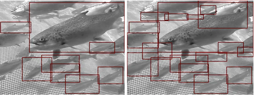
fish in each image and matching a shape model to each fish. For this purpose, 235

images of salmon in a fish farm cage were provided by AQ1 Systems Pty Ltd; fig. 4.4

shows two examples. This thesis is an extension of previous work on these images

(Williams et al., 2006). In general, the fish cage environment is less varied than many

object detection environments, but the underwater images have poor contrast and are

frequently crowded (Lines et al., 2001), which has sometimes led to the use of sonar

and laser measurements to supplement image data for fish detection (Mueller et al.,

2006). There are also many fish to detect in each image, in comparison to work such

as (Zhou & Clark, 2006), where fish are detected in a natural lake environment, but

each image is assumed to contain at most one fish.

4.2.1

Required and optional annotations

Many of the fish were faint, blurred or occluded. Some were hard to count even by a

human annotator. To train classifiers to detect them would confuse the trainer as it

tried to find features which differentiated between blurry grey net and blurry grey fish.

Therefore, only mostly (90%–100%) visible fish were used as positive training samples.

During classification, an object detector should only be expected to find objects

comparable to those in its training set. For this reason, the testing annotations it

is expected to find only contain mostly-visible fish. However, since detections on the

remaining fish are possible, and should not be counted as false positives, a separate set

of annotations was created with every fish in the image.

In total, the 119 testing images were randomly selected from the 235 provided

and annotated with 597 ‘mostly’ (90%–100%) visible fish, and 1,759 ‘partially’ (50%–

90%) visible fish. If fish from the latter set were missed they were not counted as

false negatives, but detections in their area were also not counted as false positives.

Fig. 4.5(a) is an example of mostly-visible fish annotations, while fig. 4.5(b) shows all

Figure 4.4: Example fish images

(a) Annotations for mostly-visible fish (b) Annotations for all possible fish

4.3

Seahorses

Another marine animal imaging application was to detect seahorses in tanks within

an aquaculture research facility. The intention is to detect and track seahorses over

time for behavioural analysis; ideally the seahorse poses will be found as well as their

presence. For this purpose, a seahorse tank maintained by the University of Tasmania

School of Aquaculture was filmed with a digital video camera. From this video, 263

still images were extracted, containing seahorses at two different scales. Examples of

both are shown in fig. 4.6.

Seahorses are very flexible, so their shapes vary widely. Haar Classifier Cascades

are trained on rectangular image regions, and patterns within those rectangles that are

consistent across the positive samples. Even annotating entire seahorses with

consis-tent rectangles would be difficult, and the cascade training process would have serious

difficulty finding consistent features. For these reasons, the seahorses were broken into

two segment detection problems: heads and bodies. Tails alone were still too flexible

and lacking in features, so were ignored.

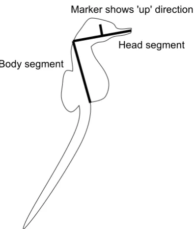
The segments were annotated by marking a line segment from the tip of the nose

to the back of the head, and from there to the base of the stomach; fig. 4.7 shows

where these points lie on a sideways-facing seahorse. The additional marker on the

head segment shows which way is ‘up’; this is ignored during evaluation but is needed

on the training images for the positive sample extraction described in section 5.2.2.

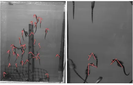
The 263 seahorse images were randomly divided into training and testing image

sets. Within the 131 testing images, 823 complete (head and body segment visible,

unoccluded and clearly connected) seahorses were marked. A second set was also

created, adding 519 partially visible or incomplete seahorses. As with the fish described

in section 4.2.1, segments and seahorses from the latter set were considered too hard

to precisely detect; even definitively annotating them was difficult. If missed they were

not counted as false negatives, but detections in their area were not counted as false

positives. Fig. 4.8(a) shows examples of the ‘required’ seahorses in two images, while

Figure 4.6: Example seahorse images

(a) Annotations for complete, visible seahorses

(b) Annotations for all possible seahorses and seahorse parts

4.3.1

Matching and merging seahorse segment detections

The neighbouring detection merging described in section 2.6.6 and the

detection-to-annotation matching described in section 2.7.2 assume that all detections and

anno-tations are in approximately the same orientation. This is not the case for seahorse

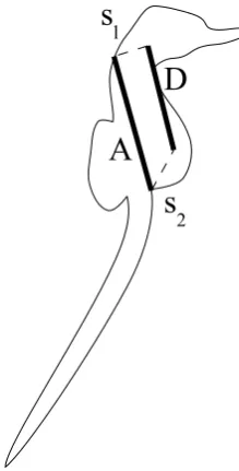
segments, which could be oriented in any direction. A new formula was therefore

cre-ated for both these situations. Given an annotationA and a detection D, it definess1

as the separation between the ‘top’ ends ofAand D, ands2 as the separation between

the ‘bottom’ ends of A and D. These properties are illustrated in fig. 4.9.

D is considered to successfully detect A if:

s1+s2 <

Alength+Dlength

2

The same formula is used when merging neighbouring detections. If two segment

detections A and D are close enough to satisfy this formula, they are placed in the

same set.

Figure 4.9: Values measured to compare a seahorse segment annotation A against a

4.4

Conclusions

This chapter has described the three image sets used in this thesis. For the face dataset,

it also explained how an existing face detection cascade was chosen. Chapter 5 will

now describe how cascades were trained on the fish and seahorse sets. All three image

sets and cascade sets will then be used in chapter 6, where Haar Classifier Cascade

confidence measures are implemented and tested. The seahorse detections made in

those two chapters are of the individual head and body segments; chapter 7 explains