Using instability to reconfigure smart structures in a spring-mass model

1

Using Instability to Reconfigure Smart Structures in a

Spring-Mass Model

Jiaying Zhang

_{and Colin R McInnes}

1 _{Department of Mechanical and Aerospace Engineering, University of Strathclyde, Glasgow, G1 1XJ,}

United Kingdom

2 _{School of Engineering, University of Glasgow, Glasgow, G12 8QQ, United Kingdom}

E-mail: [email protected]

Abstract. Multistable phenomenon have long been used in mechanism design. In this paper a subset of unstable configurations of a smart structure model will be used to develop energy-efficient schemes to reconfigure the structure. This new concept for reconfiguration uses heteroclinic connections to transition the structure between different unstable equal-energy states. In an ideal structure model zero net energy input is required for the reconfiguration, compared to transitions between stable equilibria across a potential barrier. A simple smart structure model is firstly used to identify sets of equal-energy unstable configurations using dynamical systems theory. Dissipation is then added to be more representative of a practical structure. A range of strategies are then used to reconfigure the smart structure using heteroclinic connections with different approaches to handle dissipation.

2

1. Introduction

Many structures are designed to be multi-stable equilibrium systems, so-called compliant mechanisms such as bi-stable mechanism and tri-stable mechanisms. These mechanisms store energy in some initial position and then release the stored energy through motion to another stable position [1]. For example, a discrete truss model, which consists of two bars connected by pin joints, has been investigated as a pseudo-bistable structure for morphing [2]. Others have investigated a thin-walled bi-stable geometry from natural systems and origami design principles. Finite element analysis and experimental results show the bi-stability of a reinforced silicone elastomer [3]. However, unstable equilibria could be considered to connect different configurations, as presented by Guenther, Hogg and Huberman [4]. Some special anisotropic patterning of structures can help deal with instability [5]. Moreover, active control can be used to maintain the structure in an unstable state using an agent-based approach, which controls the structure to suppress instability [6]. Such active control can in principle allow the use of heteroclinic connections to transition a smart structure between unstable states.

3

In previous work, a simple model of a smart structure was presented by McInnes and Waters [20]. The model comprised a two mass chain with three springs which were approximated to provide simple cubic nonlinearity. Then, dynamical system theory was used to investigate the characteristics of this simplified system to identify both stable and unstable equilibrium configurations, some of which were connected using heteroclinic connections. This cubic nonlinear model has also been used to investigate vibrational energy harvesting through the use of stochastic resonance [21]. The cubic model is considered as a simple mechanical system which can change its kinematic configuration between a finite set of stable or unstable equilibria. The equal energy unstable equilibria are connected through heteroclinic paths in the phase space of the problem. Therefore, in principle zero net energy is required to achieve transitions between these configurations in the absence of dissipation. Numerical results illustrated that reconfiguration between unstable equilibria can in principle be energetically efficient compared to transitions between stable configurations, which need to cross a potential barrier. In addition, a reconfiguration method based on a reference trajectory and an inverse control method has been applied to this cubic model and then extended to a more complex model for which it is difficult to generate heteroclinic connections numerically. It is envisaged that being computationally efficient, the strategy could form the basis of real-time reconfiguration of smart structures. [22].

In this paper a more complex and realistic spring-mass model is developed to consider the differences between the cubic approximation used in previous work and a real spring model with dissipation, which illustrates the possibility of using heteroclinic connections to reconfigure real smart structures, expanding on ref. [23]. Again, a set of equilibria can be found and can in principle be connected through heteroclinic paths. Then, strategies are considered to deal with the dissipation term. Two control methods are investigated, using an end-point control and an optimal control strategy. In addition, a bifurcation control strategy is investigated which allows the stability properties of the equilibria to be controlled, enabling stable equilibria to become temporarily unstable and so connected by heteroclinic paths. Numerical results are presented to illustrate the control strategies developed.

2. Smart structure model

Consider a simply clamped smart structure model, which consists of a two mass chain connected by three linear springs of stiffness (𝑘1, 𝑘2, 𝑘3) and natural lengths (𝐿1, 𝐿2, 𝐿3), as illustrated in Fig.1. It is assumed that the masses can only move in the vertical direction. If the displacement of a mass is defined by 𝒙(𝑥1, 𝑥2), while the spring clamps are separated by 3𝑑, it can be shown that the spring lengths after deformation are described by

4

𝑙2= √((𝑥1− 𝑥2)2+ 𝑑2) (2)

𝑙3= √(𝑥22+ 𝑑2) (3)

x1 x2

k1

k2

k3

m m

d d d

β β

Figure 1. 2 degree-of-freedom bucking beam model with damping coefficient 𝛽.

In order to investigate the characteristics of the system, it is assumed that the structure can initially be considered as a Hamiltonian system (without dissipation) with a simplification of unit mass 𝑚. From Fig. 1, the Hamiltonian for this system can then be defined from the kinetic and potential energy with spring natural length 𝑳(𝐿1, 𝐿2, 𝐿3) through Eqs. (4) and (5)

𝑇(𝒑) =1 2(𝑝1

2_{) +}1

2(𝑝2

2_{) (4)}

𝑉(𝒙, 𝑳) =1

2𝑘1(𝑙1− 𝐿1)

2₊1

2𝑘2(𝑙2− 𝐿2)

2₊1

2𝑘3(𝑙3− 𝐿3)

2 ₍₅₎

with momentum coordinates 𝒑(𝑝1, 𝑝2) associated with position coordinates 𝒙(𝑥1, 𝑥2).

However, for a realistic model dissipation must also be considered, which of course will destroy the Hamiltonian structure of the dynamics. Therefore, phase trajectories from one unstable equilibrium point cannot reach another equal-energy unstable equilibrium point. In order to compensate for such dissipation, controllers need to be used to ensure that heteroclinic connections exist. Therefore, the dynamics of the problem can be extended by the addition of linear dissipation parameterised by 𝛽, as shown in Fig.1.

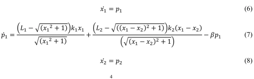
The problem can now fully defined by a dynamical system of the form

𝑥1̇ = 𝑝1 (6)

𝑝̇1=

(𝐿1− √(𝑥12+ 1))𝑘1𝑥1

√(𝑥12+ 1)

+(𝐿2− √((𝑥1− 𝑥2)

2_{+ 1))𝑘}

2(𝑥1− 𝑥2)

(√(𝑥1− 𝑥2)2+ 1)

− 𝛽𝑝1 (7)

5 𝑝̇2 =

(𝐿3− √(𝑥22+ 1))𝑘3𝑥2

√(𝑥22+ 1)

−(𝐿2− √((𝑥1− 𝑥2)

2_{+ 1))𝑘}

2(𝑥1− 𝑥2)

(√(𝑥1− 𝑥2)2+ 1)

− 𝛽𝑝2 (9)

Then, using dynamical system theory to analyse the system defined by Eqs. (6-9), it can be shown that there exists a number of both stable and unstable equilibria which may be connected in phase space. One such type of path is the heteroclinic connection, which requires that the stable and unstable manifolds of two equal-energy unstable equilibria are connected. Solving Eqs. (6) to (9) for equilibrium solutions yields 13 equilibria for the parameter set, 𝑘1= 𝑘2= 𝑘3= 1, 𝑑 = 1, 𝐿1= 𝐿2 = 𝐿3 = 2.5. The details of the equilibria are listed in Table 1.

Moreover, the stability properties of these equilibria can be determined from the Hessian matrix of the potential energy. In the second derivative test for determining extrema of the potential function 𝑉(𝒙, 𝑳), the discriminant D is given by

𝐷 = || 𝜕2𝑉 𝜕𝑥₁2

𝜕2𝑉 𝜕𝑥1𝜕𝑥2

𝜕2_𝑉

𝜕𝑥2𝜕𝑥1

𝜕2_𝑉

𝜕𝑥₂2

|

| ₍₁₀₎

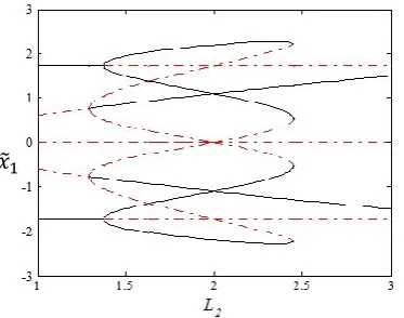
Through using the second derivative test discriminant [23], it can be shown that the system possesses 1 unstable equilibrium E0 with a global potential maximum, 6 stable equilibria E1 to E6 with a global potential minimum and 6 unstable equilibria E7 to E12 where the potential has a saddle, as can be seen in Fig. 2. The corresponding shapes of the structure are shown in Fig. 3, which presents different configurations associated with each of the 13 equilibria. Meanwhile, it can be seen from Table 1 and Fig. 2 that E0 has the highest potential V with each spring in compression while E7 to E12 are unstable equilibria which have only one spring in compression and the stable equilibria E1 to E6 have both springs extended.

6

E0 0 0 3.38 1.75 Maximum

E1 1.48 -1.48 0.70 1.35 Minimum

E2 -1.48 -2.96 0.70 1.35 Minimum

E3 -2.96 -1.48 0.70 1.35 Minimum

E4 -1.48 1.48 0.70 1.35 Minimum

E5 1.48 2.96 0.70 1.35 Minimum

E6 2.96 1.48 0.70 1.35 Minimum

E7 0 2.29 1.13 -1.81 Saddle

E8 2.29 2.29 1.13 -1.81 Saddle

E9 2.29 0 1.13 -1.81 Saddle

E10 0 -2.29 1.13 -1.81 Saddle

E11 -2.29 -2.29 1.13 -1.81 Saddle

E12 -2.29 0 1.13 -1.81 Saddle

Figure 2. Potential 𝑉(𝒙, 𝑳)and equilibria (6 stable equilibria E1 to E6, and 6 unstable equilibria

E7 to E12). (a) 3D surface plot. (b) Contour plot.

E0

a

b

c

E1 E2 E3

E5 E6

E4

E7 E9

E12

E10

E8

E11

Figure 3. Equilibria for a two mass chain with (a) maximum potential equilbria E0 (b) stable

equilbria E1-6 and (c) unstable equilibria E7-12.The unstable equilibria have equal potential V. x2

x1

V

x1

x2

7

Using dynamical system theory, we can then generate the stable and unstable manifolds of the unstable equilibria to seek possible connections between them [24]. For the conservative system, linearisation of Hamilton’s equations in the neighbourhood of each equilibrium point yields pairs of positive and negative eigenvalues with the corresponding eigenvectors for the stable and unstable direction 𝒖𝒔and

𝒖𝒖 associated with each eigenvalue. These eigenvectors 𝒖𝒔and 𝒖𝒖 are tangent to the stable manifold

Ws and the unstable manifold Wu in the neighbourhood of each equilibrium [20]. Therefore, the eigenvectors can be mapped to approximate the stable and unstable manifolds by integrating forwards or backwards from an unstable equilibrium point 𝒕𝒆, defined by

𝒕𝒔_{= 𝒕}𝒆_{+ 𝜖𝒖}𝒔 ₍₁₁₎

𝒕𝒖_{= 𝒕}𝒆_{+ 𝜖𝒖}𝒖 ₍₁₂₎

for 𝜖 ≪ 1𝒕 = (𝒙, 𝒑) ∈ 𝐑4. While this method can be used to find heteroclinic connections between equal-energy unstable equilibria, a means to stabilise the structure before and after such a reconfiguration must firstly be sought.

3. Bifurcation Control

In previous work [23], a numerical search technique for reconfiguration using heteroclinic connections without dissipation was investigated. It was assumed that the instability of the equal-energy unstable equilibria could be compensated by using active control. However, an alternative bifurcation control method may be considered if the natural length of the springs 𝐿1−3 can be manipulated, for example if the springs are manufactured from an appropriate shape memory alloy. A conservative Hamiltonian system is assumed initially, with compensation for dissipation considered later in Section 4.

8

Figure 4. Schematic representation of bifurcation control (a) and (c) are different locally stable configurations of the structure (b) heteroclinic connection between the two equal-energy unstable configurations.

Based on this simple illustrative model, a new reconfigurable strategy is investigated using the spring-mass smart structure model detailed in Section 2.

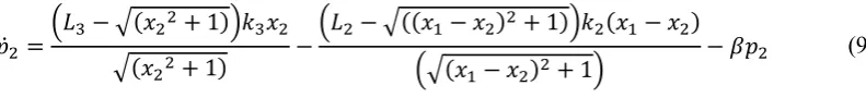
In order to illustrate this strategy directly, 𝐿2 is firstly manipulated and changed from 1 to 2.5 with 𝐿1 and 𝐿3 fixed. Initially a large change in the spring natural length is considered for clarity of illustration; a smaller change will be used later. It can be seen from Fig. 5 that the number of equilibria will change with an increase of 𝐿2, which is shown by the equilibria 𝑥̃1 at different lengths of 𝐿2. Moreover, there

are three invariant points (0, 0), (√3, √3) and (−√3, −√3) whose locations are independent of 𝐿2. For 𝐿2 = 1 the equilibria 𝐸1 and 𝐸2 are stable, and the potential forms local minima at these

locations, as shown in Fig. 6. Then, if 𝐿2 is increased such that 𝐿2≥ 2, the equilibria (√3, √3) and

(−√3, −√3) became unstable and a heteroclinic connection can be used to reconfigure the structure between these two equilibria, as shown in Fig. 7. After the reconfiguration, 𝐿2 is finally decreased

such that 𝐿2= 1 and the system becomes stable again. This scheme allows operation of the structure in a stable state, a transition to instability to reconfigure the structure, and then continued operation in another stable state.

Figure 5. Bifurcation diagram for the spring-mass model. Projection of the location of the equilibria onto the 𝑥1 axis for𝐿1= 2 , 𝐿3= 2 and 1 ≤ 𝐿2≤ 3. Solid line: stable equilibria, dashed line: unstable equilibria.

9

Figure 6. Effective potential 𝑉(𝒙, 𝑳) with 𝐿₁=2, 𝐿₂=1 and 𝐿₃=2. 𝐸₁ and 𝐸₂ are stable, 𝐸₃

and 𝐸4 are unstable.

Figure 7. Effective potential 𝑉(𝒙, 𝑳) with 𝐿1=2, 𝐿2=2.5 and 𝐿3=2. 𝐸1 and 𝐸2 are unstable,

𝐸₃ and 𝐸₄ are stable.

A transition using this scheme (without dissipation) is shown in Fig. 8. The coupling parameters are

𝐿1=2 and 𝐿3=2 with 𝐿2 switched from 2.5 to 1 to manipulate the stability properties of 𝐸1 and 𝐸2. Firstly, a small displacement is added to the system in the local minimum potential well to demonstrate capture at the equilibrium point. This initial oscillation of the system in the potential well at 𝐸1 with

𝐿2= 1 can be seen, followed by a transition to 𝐸2 with 𝐿2= 2.5 after the bifurcation and then a return to oscillation in the local minimum potential well at 𝐸2 with 𝐿2= 1.

x

1 x2

-3 -2 -1 0 1 2 3

-3 -2 -1 0 1 2 3

E₄ E₃

E₁

E₂

E

0

x₁ x2

-3 -2 -1 0 1 2 3

-3 -2 -1 0 1 2 3

E₀

E₁

E₂ E₃

10

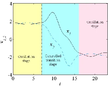
Figure 8. Controlled transition from 𝐸₁ at (√3, √3 )to 𝐸₂ at (−√3, −√3 ) with bifurcation control. The coupling parameters 𝐿₁=2 and 𝐿₃=2 with 𝐿₂ switched from 2.5 to 1 to manipulate the stability properties of 𝐸1 and 𝐸2.

In order to further explore the possibility of reconfiguring the smart structure using bifurcation control,

a more complex situation will now be considered. Figure 2 and 5 show that the equilibria (√3, √3) and

(−√3, −√3) became unstable when 𝐿2= 2, but with the same potential energy as other saddle points

such as (0, √3). An iterative approach [25], can also be used which divides a position coordinate, such as 𝑥1, into several steps with a desired increment, then the other position coordinate 𝑥2 can be used to seek to minimize the potential energy of every step. Therefore, an ideal path can be generated on the

potential energy contour from (√3, √3) to (−√3, −√3) with 𝐿1= 𝐿2= 𝐿3 = 2. This results in a

series of connected heteroclinic connections between (√3, √3) and (−√3, −√3), as shown in Fig. 9. Therefore, we can consider using the bifurcation control method to reconfigure the structure in a more realistic way with a smaller change of the spring natural length such that 𝐿2 switches from 2 to 1.3.

Figure 9. Potential energy contour plot and ideal path from (√3, √3 ) to (−√3, −√3 ).

x₁ x2

-2 -1 0 1 2

11

Figure 10 shows the transition (without dissipation) using this modified bifurcation control. The coupling parameters are 𝐿1= 2 and 𝐿3= 2 with 𝐿2 switched from 2 to 1.3 to manipulate the stability properties of 𝐸1 and 𝐸2. Then, a small displacement is again added to the system in the local minimum potential well to demonstrate capture at the equilibrium point. The initial oscillation of the

system in the potential well at 𝐸1 with 𝐿2= 1.3 can therefore be seen, followed by a transition to 𝐸2 with 𝐿2 = 2 and then a return to oscillation in the local minimum potential well at 𝐸2 with 𝐿2= 1.3. In addition, the switch process is a simple step change of 𝐿2 from 1.3 to 2, as shown in Fig. 11.

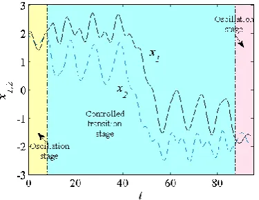
Figure 10. Controlled transition from 𝐸₁ at (√3, √3 )to 𝐸₂ at (−√3, −√3 ) with bifurcation control with 𝐿₂ switched from 1.3 to 2 to manipulate the stability properties of 𝐸₁ and 𝐸₂.

Figure 11. A step change of 𝐿₂ (1.3 to 2) during the bifurcation control.

12

of bifurcations in this type of nonlinear system. Therefore, an easily visualized means (e.g. natural length of the springs) are used to achieve the reconfiguring process.

4. Controlled heteroclinic connections in a dissipative system

As noted earlier, dissipation needs to be considered for a realistic model where Eq. (4) and (5) show the

total energy 𝑊 = 𝑇 + 𝑉 of the system is monotonically decreasing as 𝑊̇ = −𝛽(𝑝12+ 𝑝22) corresponding to the general condition 𝑝1 ≠ 0, 𝑝2 ≠ 0. In order to proceed it will be assumed that each spring can now be manipulated with variations of the real spring length ∆𝐿 by using smart materials such as shape memory polymers, so from Eq. (7) and (9) it can be seen that

𝑝̇1𝑝1−

((𝐿1+ ∆𝐿1) − √(𝑥12+ 1)) 𝑘1𝑥1

√(𝑥12+ 1)

𝑝1

−((𝐿2+ ∆𝐿2) − √((𝑥1− 𝑥2)

2_{+ 1)) 𝑘}

2(𝑥1− 𝑥2)

( √(𝑥1− 𝑥2)2+ 1)

𝑝1= −𝛽𝑝12

(13)

𝑝̇2𝑝2−

((𝐿3+ ∆𝐿3) − √(𝑥22+ 1)) 𝑘3𝑥2

√(𝑥22+ 1)

𝑝2

+((𝐿2+ ∆𝐿2) − √((𝑥1− 𝑥2)

2_{+ 1)) 𝑘}

2(𝑥1− 𝑥2)

( √(𝑥1− 𝑥2)2+ 1)

𝑝2= −𝛽𝑝22

(14)

which can be written as

𝑑

𝑑𝑡(𝑇 + 𝑉) = −𝛽𝑝1

2₊ ∆𝐿1𝑘1𝑥1

√(𝑥12+ 1)

𝑝1− 𝛽𝑝22+

∆𝐿3𝑘3𝑥2

√(𝑥22+ 1)

𝑝2

+ ∆𝐿2𝑘2(𝑥1− 𝑥2) ( √(𝑥1− 𝑥2)2+ 1)

(𝑝1− 𝑝2)

(15)

13

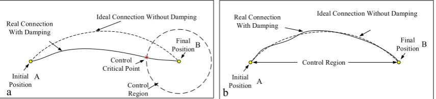
Conversely, the continuous strategy can be controlled by constantly monitoring and controlling states during the reconfiguration of the smart structure, as shown in Fig. 12b.

Initial PositionA Final PositionB Control Region Control Critical Point

Ideal Connection Without Damping Real Connection With Damping Initial Position A Final PositionB Ideal Connection Without Damping Real Connection

With Damping

Control Region

Figure 12. Control strategy (a) End-point control (b) Continuous control.

End-point control

In order to ensure convergence to some equilibrium point (𝑥̃₁, 𝑥̃2) a Lyapunov function is defined such that

𝜙(𝒙, 𝑳) =1 2𝑝1

2₊1

2𝑝2

2₊1

2(𝑥1− 𝑥̃1)

2₊1

2(𝑥2− 𝑥̃2)

2 (16)

where 𝜙(𝒙, 𝑳) > 0 and 𝜙(𝑥̃1, 𝑥̃2) = 0. The time derivative of the Lyapunov function is clearly

𝜙̇(𝒙, 𝑳) = 𝑝1(𝑝̇1+ (𝑥1− 𝑥̃1)) + 𝑝2(𝑝̇2+ (𝑥2− 𝑥̃2)) (17)

Then, substituting from the Eq. (7) and (9) the controller for 𝐿1, 𝐿2 and 𝐿3can be defined as

𝐿1= −

√(𝑥12+ 1)

𝑘1𝑥1

(𝜂𝑝1+ (𝑥1− 𝑥̃1) −

(𝐿2− √((𝑥1− 𝑥2)2+ 1))𝑘2(𝑥1− 𝑥2)

(√(𝑥1− 𝑥2)2+ 1)

− 𝑘1𝑥1) (18)

𝐿2 = −

√(𝑥1− 𝑥2)2+ 1

𝑘2(𝑥1− 𝑥2)

(𝜂𝑝1+ (𝑥1− 𝑥̃1) +

(𝐿1− √(𝑥12+ 1))𝑘1𝑥1

√(𝑥12+ 1)

− 𝑘2(𝑥1− 𝑥2)) (19)

𝐿3= −

√(𝑥22+ 1)

𝑘3𝑥2

(𝜂𝑝2+ (𝑥2− 𝑥̃2) −

(𝐿2− √((𝑥1− 𝑥2)2+ 1))𝑘2(𝑥1− 𝑥2)

(√(𝑥1− 𝑥2)2+ 1)

− 𝑘3𝑥2) (20)

for some control parameter 𝜂. It is noted that the system has 2 state variables 𝑥1 and 𝑥2, which can select two controllers from 𝐿1, 𝐿2 and 𝐿3as control variables to avoid singularities. For example, since 𝑘2(𝑥1− 𝑥2) ≠ 0, 𝑘3𝑥2 ≠ 0 in the neighbourhood of the required equilibrium point 𝐸10, 𝐿2 and 𝐿3 are selected as controllers in the neighbourhood of that point.

It can then be seen that 𝜙 is monotonically decreasing such that

14

𝜙̇(𝒙, 𝑳) = −(𝜂 + 𝛽)(𝑝12+ 𝑝22) ≤ 0 (21)

and so 𝒙 → (𝑥̃1, 𝑥̃2) and 𝒑 → (0,0) within the neighbourhood of target point.

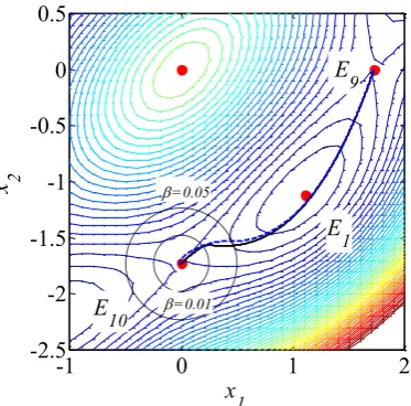
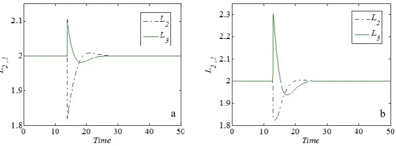
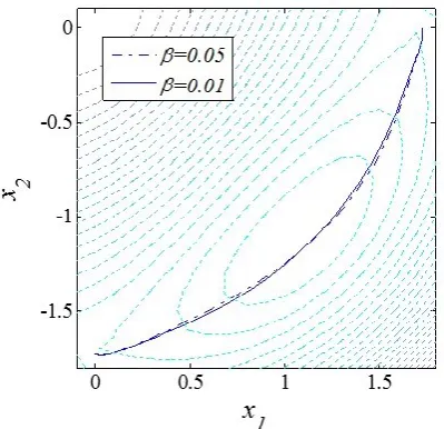
An example of controlled heteroclinic connections for 𝛽 = 0.01 and 𝛽 = 0.05 are shown in Fig. 13 for a reconfiguration between E9 and E10. To initiate the heteroclinic connection, a displacement along the unstable manifold of E9 is preformed and the controller will be activated when the phase space path is in the defined neighbourhood R of E10 (𝜂 = 3). The corresponding controls 𝐿2 and 𝐿3 are shown in Fig. 14. It can be seen that the controls are only active when the phase space path is in the end-point region of E10. Numerical results demonstrate that the control effort grows with increasing dissipation parameter 𝛽. That is, the control region needs to be enlarged to fit the increasing dissipation parameter

𝛽 as shown in Fig. 13.

Figure 13. Controlled transition from E9 at (1.732051,0) to E10 at (0,-1.73205) with the controller

active in the neighbourhood of E10 with different dissipation. Solid line: dissipation parameter 𝛽 = 0.01, dashed line: dissipation parameter 𝛽 = 0.05.

-1 0 1 2

-2.5 -2 -1.5 -1 -0.5 0 0.5

x₁

x 2

=0.01

=0.05

E₁₀

15

Figure 14. Controlled transition from E9 at (1.732051, 0) to E10 at (0, -1.73205) with the controls

actuated through L2 and L3in the neighbourhood of E10. (a) Dissipation parameter 𝛽 = 0.01. (b)

Dissipation parameter 𝛽 = 0.05.

Continuous control

For comparison with the end-point control strategy, a continuous control method is now investigated to approximate the heteroclinic connection. This problem is revisited as a computational optimal control problem to determine the control histories which meet the boundary conditions of the problem. In addition to satisfying the state boundary conditions, these control histories also need to minimise a performance index function. Then, the optimal tool PSOPT is employed to solve this optimal control problem numerically using the direct method. PSOPT is coded in C++ by Becerra [26] and is free and open source. The code can deal with many numerical optimisation problems, in particular with endpoint constraints, path constraints, and interior point constraints. Moreover, it can solve the non-linear programming (NLP) problem by using IPOPT, which is an interior point method for large-scale problems.

The system can be considered under quasi-static conditions, so that the energy required for each controller can be defined as

𝐸 =1 2𝑘(∆𝐿)

2 ₍₂₂₎

where 𝑘 is the spring stiffness and ∆𝐿 is variation of the spring natural length. Therefore, the performance index of the system can be defined

𝐽 = ∫ ((∆𝐿1)2+ (∆𝐿2)2+ (∆𝐿3)2)𝑑𝑡 𝑡𝑓

0

(23)

16

where 𝑡𝑓 means the duration from initial condition to the final condition, then, we define conditions

for a transition from the unstable equilibrium E9 to E10 as

[𝒙(0) 𝒙(T) 𝒙̇(0) 𝒙̇(T)] = [1.732 0 0 0

0 −1.732 0 0] (24)

The numerical results for dissipation parameters 𝛽 = 0.01 and 𝛽 = 0.05 are shown in Fig. 15. The corresponding controls 𝐿1, 𝐿2 and 𝐿3 are shown in Fig. 16. It can be seen that the controls are symmetric about the point 𝑡 = 𝑇 2⁄ as expected. Moreover, in general more energy is required to compensate for a larger dissipation parameter 𝛽, which means the range of the controller becomes larger for the reconfiguration, as shown in Fig 16.

Figure 15. Controlled transition from E9 at (1.732051,0) to E10 at (0,-1.73205) with the controller

active under the continuous control method(dissipation parameters 𝛽 = 0.01, 0.05).

Figure 16. Controlled transition from E9 at (1.732051,0) to E10 at (0,-1.73205) with the controls

actuated through L1,L2 and L3 under the continuous control method. (a) Dissipation parameters 𝛽 = 0.01 (b) Dissipation parameter 𝛽 = 0.05.

0 1 2 3 4 5 6 7 8 9 10

1.85 1.9 1.95 2 2.05 Time L₁

0 1 2 3 4 5 6 7 8 9 10

1.95 2 2.05 2.1 2.15 Time L₂

0 1 2 3 4 5 6 7 8 9 10

1.9 1.95 2 2.05 Time L₃

0 1 2 3 4 5 6 7 8 9 10

1.85 1.9 1.95 2 2.05 Time L₁

0 1 2 3 4 5 6 7 8 9 10

1.95 2 2.05 2.1 2.15 Time L₂

0 1 2 3 4 5 6 7 8 9 10

1.9 1.95 2 2.05 Time L₃

17

In order to keep the structure model simple, some assumptions and simplifications were proposed to implement the research, for example, the dissipation was assumed as linear relationship. The model used in this paper has some differences with a real structural model, omitting material viscosity, time lag effects of the control. Through using this qualitatively simple model, new insights can be obtained on the use of heteroclinic connections. This simple model can be used to introduce this new reconfiguration concept and provide insights for use in a more accurate high fidelity model [27]. Although the end-point control method is easy, it needs an instantaneous control in the reconfiguration procedure. Besides, most importantly, it may be difficult to find exact heteroclinic connections numerically in complex nonlinear dynamic systems. In contrast, the continuous control method could provide a more smooth controlled transitions with less energy, but it may be computationally intensive to determine. Therefore, a smart structure can be reconfigured from one unstable state to another through choosing a suitable control maneuver from the end-point control and the continuous control method. In addition, the utilisation of these two methods can be clarified for different systems, for example, the end-point method could be adequate for lightly damped systems and the continuous control methods can provide satisfactory state trajectories with small changes in control variables.

Moreover, a better reconfigurable strategy is used to combine bifurcation control and controlled heteroclinic connections, which is expected to reconfigure real smart structures between stable states. For example, structures are assumed initially in local stable states. Through performing bifurcation the local condition becomes unstable. Then, bifurcation is performed again when end-point control generates a trajectory to the target equilibrium point. This represents a computationally efficient way to achieve reconfiguration for smart structures between two different equilibria positions with less energy.

5. Conclusion

18

the problem which can be exploited to develop the concept towards the reconfiguration of real smart structures.

Acknowledgments

McInnes was support by a Leverhulme Trust Fellowship and a Royal Society Wolfson Research Merit Award.

References

[1] Howell L L, Magleby S P and Olsen B M 2013 Handbook of Compliant Mechanisms (John Wiley & Sons)

[2] Brinkmeyer a., Pirrera a., Santer M and Weaver P M 2013 Pseudo-bistable pre-stressed morphing composite panels Int. J. Solids Struct.50 1033–43

[3] Daynes S, Grisdale A, Seddon A and Trask R 2014 Morphing structures using soft polymers for active deployment Smart Mater. Struct.23 012001

[4] Guenther O, Hogg T and Huberman B A 1997 Controls for unstable structures Smart Structures and Materials 1997: Mathematics and Control in Smart Structures, The Society of Photo-Optical Instrumentation Engineers (SPIE) conf. (June); Proc.SPIE pp 754–63

[5] Lee D-Y, Kim J, Kim J-S, Baek C, Noh G, Kim D-N, Kim K, Kang S and Cho K-J 2015 Anisotropic Patterning to Reduce Instability of Concentric-Tube Robots IEEE Trans. Robot.31 1311–23

[6] Hogg T and Huberman B A 1998 Controlling smart matter Smart Mater. Struct.7 R1–14

[7] Terrence J, Mary F and Farhan G 2009 A bistable mechanism for chord extension morphing

rotors. SPIE Smart Structures and Materials Nondestructive Evaluation and Health Monitoring

(International Society for Optics and Photonics) pp 72881C1–12

[8] Lu K-J and Kota S 2003 Design of Compliant Mechanisms for Morphing Structural Shapes J. Intell. Mater. Syst. Struct.14 379–91

[9] Camescasse B, Fernandes A and Pouget J 2013 Bistable buckled beam: Elastica modeling and analysis of static actuation Int. J. Solids Struct.50 2881–93

[10] Camescasse B, Fernandes A and Pouget J 2014 Bistable buckled beam and force actuation: Experimental validations Int. J. Solids Struct.51 1750–7

[11] Lagoudas D C 2008 Shape Memory Alloys: Modeling and Engineering Applications (New York: Springer)

[12] Flatau A B and Chong K P 2002 Dynamic smart material and structural systems Eng. Struct.24 261–70

[13] Mohd Jani J, Leary M, Subic A and Gibson M a. 2014 A review of shape memory alloy research, applications and opportunities Mater. Des.56 1078–113

[14] Behl M, Kratz K, Zotzmann J, Nöchel U and Lendlein A 2013 Reversible bidirectional shape-memory polymers Adv. Mater.25 4466–9

19

[16] Hurlebaus S and Gaul L 2006 Smart structure dynamics Mech. Syst. Signal Process.20 255–81 [17] Tolley M T, Felton S M, Miyashita S, Aukes D, Rus D and Wood R J 2014 Self-folding origami:

shape memory composites activated by uniform heating Smart Mater. Struct.23 094006 [18] Felton S, Tolley M, Demaine E, Rus D and Wood R 2014 A method for building self-folding

machines Science (80-. ).345 644–6

[19] Hawkes E, An B, Benbernou N M, Tanaka H, Kim S, Demaine E D, Rus D and Wood R J 2010 Programmable matter by folding. Proc. Natl. Acad. Sci. U. S. A.107 12441–5

[20] McInnes C R and Waters T J 2008 Reconfiguring smart structures using phase space connections

Smart Mater. Struct.17 025030

[21] McInnes C R, Gorman D G and Cartmell M P 2008 Enhanced vibrational energy harvesting using nonlinear stochastic resonance J. Sound Vib.318 655–62

[22] Zhang J and McInnes C R 2015 Reconfiguring smart structures using approximate heteroclinic connections Smart Mater. Struct.24 105034

[23] Zhang J and McInnes C R 2015 Reconfiguring Smart Structures using Approximate Heteroclinic Connections in A Spring-Mass Model Proceedings of the ASME Conference on Smart Materials, Adaptive Structures and Intelligent Systems (SMASIS 2015) (Colorado Springs)

[24] Wiggins S 1990 Introduction to applied nonlinear dynamical systems and chaos (New York: Springer)

[25] Oh Y S and Kota S 2009 Synthesis of multistable equilibrium compliant mechanisms using combinations of bistable mechanisms J. Mech. Des.131 021002

[26] Becerra V M 2010 Solving complex optimal control problems at no cost with PSOPT 2010 IEEE Int. Symp. Comput. Control Syst. Des. 1391–6