Effect of frequency domain attributes of wavelet analysis filter banks for structural damage localization using the relative wavelet entropy index

City, University of London Institutional Repository

Citation

: Gkoktsi, K. & Giaralis, A. (2015). Effect of frequency domain attributes of

This is the accepted version of the paper.

This version of the publication may differ from the final published

version.

Permanent repository link:

Link to published version

: http://dx.doi.org/10.1504/IJSMSS.2015.078365

Copyright and reuse:

City Research Online aims to make research

outputs of City, University of London available to a wider audience.

Copyright and Moral Rights remain with the author(s) and/or copyright

holders. URLs from City Research Online may be freely distributed and

linked to.

Effect of frequency domain attributes of wavelet analysis filter banks

for structural damage localization using the relative wavelet entropy

index

Authors

K. Gkoktsi1, A. Giaralis1* Affiliations

1_{Department of Civil Engineering, City University London, Northampton Square, EC1V} 0HB, London, UK

Abstract

A novel numerical study is undertaken to assess the influence of the frequency domain (FD) attributes of wavelet analysis filter banks for vibration-based structural damage detection and localization using the relative wavelet entropy (RWE): a damage-sensitive index derived by wavelet transforming linear response acceleration signals from a healthy/reference and a damaged state of a given structure subject to broadband excitations. Four different judicially defined energy-preserving wavelet analysis filter banks are employed to compute the RWE pertaining to two benchmark structures via algorithms which can efficiently run on wireless sensors for decentralized structural health monitoring. It is shown that filter banks of compactly supported in the FD wavelet bases (e.g., Meyer wavelets and harmonic wavelets) perform significantly better than the commonly used in the literature dyadic Haar discrete wavelet transform filter banks since they achieve enhanced frequency selectivity among scales (i.e., minimum overlapping of the frequency bands corresponding to adjacent scales) and, therefore, reduce energy leakage and facilitate the interpretation of numerical results in terms of scale/frequency dependent contributors to the RWE. Moreover, it is demonstrated that dyadic DWT filter banks with large constant Q values (i.e., ratio of effective frequency over effective bandwidth) are better qualified to capture damage information associated with high frequencies. Finally, it is concluded that wavelet analysis filter banks achieving non-constant Q analysis are most effective for RWE-based stationary damage detection as they are not limited by the dyadic DWT discretization and can target the structural natural frequencies in cases these are a priori known.

Keywords: structural health monitoring; damage detection; relative wavelet entropy; wavelet filter banks.

1. Introduction and motivation

Vibration-based structural health monitoring (VSHM) techniques are commonly employed to detect and to localize damage in engineering structures and structural components due to degradation over time under operational conditions, or due to extreme/accidental events and loading (e.g., Doebling et al. 1998). VSHM relies on acquisition and processing of structural response acceleration signals recorded by sensors (accelerometers) placed on vibrating structures which are excited by dynamic (i.e., time-varying) or impulsive forces. Whether ambient (operational) or purposely induced, the excitation forces for VSHM should, ideally, have a low amplitude, such that structures vibrate in the linear regime, and a flat Fourier spectrum over a sufficiently wide range of frequencies, such that an adequate number of (linear) modes of vibration are excited (e.g., Ewins 2000, Reynders 2012). Then, global damage detection and even localization of damage (in densely instrumented structures) are achieved by observing changes to the values of damage-sensitive indices derived from linear response acceleration signals acquired at the current (potentially damaged) state of a structure with those pertaining to a past (reference or “healthy”) structural state (e.g., Worden et al. 2007). These damage-sensitive indices may coincide with the dynamic/modal properties (e.g., natural frequencies) or mechanical properties (e.g., stiffness coefficients) of the monitored structure, or be derived from them (e.g., modal curvatures, strain energy, etc.) (e.g., Humar et al. 2006). Alternatively, data-driven damage indices, not amenable to any physical/structural interpretation (but related to the physics of the problem), have also been considered in conjunction with statistical signal processing techniques for the purpose at hand. Damage detection approaches based on the latter indices are sometimes more effective since they employ computational tools not considered in standard linear structural dynamics approaches, such as the wavelet transform (WT) (e.g., Yen and Lin 2000, Sun and Chang 2004), while they are not limited by physical considerations.

time-scale plane by projecting it onto a collection of double-indexed localized in time oscillatory functions (wavelets) generated by scaling and translating in time a single “mother” wavelet function (e.g. Daubechies 1992). Depending on the properties of the mother wavelet, each scale considered in the WT can be assigned an effective (central) frequency and an effective bandwidth. In this regard, if an energy-preserving analysing wavelet basis is used, the squared magnitude of the WT maps the energy of a signal on the time-frequency plane (see also Cohen 1995). Under this condition, the damage detection capability of the RWE relies on detecting changes to the energy distribution of (or to the information carried by) response acceleration signals between the healthy and the damaged state across the different scales considered in the WT spanning certain frequency bands. Indeed, the definition of the RWE is closely related to the Shannon wavelet entropy introduced by Blanco et al. (1998) for signal characterization in certain biomedical applications, based on the information carried by the WT in time and in frequency.

Ren and Sun (2008) verified the potential of the RWE to serve as a damage-sensitive index by considering experimental data pertaining to a beam and to a composite bridge excited by impulsive/hammer force. In computing the RWE, the authors considered a non-smooth Daubechies (or Haar) wavelet basis implemented in a wavelet analysis digital filter bank yielding a quite efficient to compute discretized version of the WT, the so-called discrete wavelet transform (DWT) (e.g. Daubechies 1992, Goswami and Chan 1999). Recognizing the potential of the RWE for damage detection in practical VSHM applications, Yun et al. (2011) considered arrays of battery operated wireless sensors computing locally on on-board micro-processors the DWT and, thus, being able to derive the RWE in a decentralized computationally-efficient manner aiming to reduce the power consumption of sensors and, therefore, to prolong their battery life: a very important practical consideration in cost-effective VSHM using wireless sensor networks (Lynch 2007). More recently, Lee et al. (2014) adopted the RWE to detect faulty/damaged connections in pin-jointed truss structures by considering healthy connections as a reference (healthy state), and processing signals recorded at all healthy and faulty connections acquired from a single vibration test.

a shift of the natural frequencies due to damage. In this regard, it is natural to expect that the use of wavelet bases (or, equivalently, wavelet analysis filter banks) capable of resolving fine differences in the signal energy distribution in the frequency domain, or among the wavelet analysis scales, renders the RWE more effective for stationary damage detection. However, the Haar (non-smooth Daubechies) wavelet filter bank employed by Ren and Sun (2008) to compute the RWE is known to have significant overlapping between the frequency bands corresponding to different wavelet analysis scales (e.g., Vetterli and Herley 1992). Indeed, Yun et al. (2011) reported the problem of signal energy leakage among wavelet scales (spectral leakage) in using Haar wavelets for RWE-based damage detection, which renders the interpretation of the RWE values a challenging task. Further, in the above work, limited results using a smooth (higher-order) Daubechies wavelet filter bank, which attains improved frequency resolution attributes compared to the Haar wavelet basis, were provided and the authors noted that the use of different analysis wavelets influences the obtained RWE values. However, the authors neither did they attempt any direct comparison between different wavelet filter banks, nor did they provide recommendations to indicate a preferable wavelet filter bank. Moreover, despite being computationally efficient, the standard dyadic (octave) frequency domain discretization of the DWT used in Ren and Sun (2008) and Yun et al. (2011) does not facilitate a detailed characterization of high frequency content. This limitation may hinder damage detection and localization based on changes to the energy of response acceleration signals related to the higher modes of vibration (e.g., Yen and Lin 2000). The continuous wavelet transform (CWT) considered by Lee et al. (2014) may overcome the latter limitation, but at the expense of significant computational cost which may not be cost-efficient to be accommodated by wireless sensors.

same. To this aim, the Meyer wavelet basis for DWT (e.g., Misiti et al. 2000) and the harmonic wavelet basis (Newland 1994) are herein considered, for the first time in the literature, alongside smooth and non-smooth Daubechies wavelet bases to gauge their effectiveness for RWE-based damage detection by examining scale or frequency dependent contributions to the RWE index vis-à-vis. All four considered wavelet bases can be efficiently computed using either standard wavelet filter banks of finite impulse response filters or fast Fourier Transform (FFT)-based algorithms. Notably, wireless sensors with on-board processors able to perform these standard signal processing operations are available (Lynch 2007).

The remainder of this paper is organized as follows. Section 2 provides a concise background on the WT focusing on energy preserving wavelet analysis filter banks, while section 3 reviews the RWE for stationary structural damage detection. Next, section 4 presents the four different wavelet analysis filter banks considered in this work and discusses their frequency domain attributes. Finally, section 5 furnishes novel numerical data for RWE-based damage detection using different wavelet filter banks pertaining to two different benchmark structures excited by stationary and non-stationary broadband forcing functions, while section 6 summarizes concluding remarks and points to future work.

2. A review on the wavelet transform and energy preserving wavelet analysis filter

banks

2.1.The continuous wavelet transform (CWT)

Consider a real signal x(t) of finite energy E in the axis of time t,or in time domain (TD), expressed by

2 ₁ 2

( ) ( ) .

2

E x t dt X ω dω

π

∞ ∞

−∞ −∞

=

∫

∫

In the above equation, X(ω) is the complex-valued continuous-time Fourier transform (CTFT) defined by

( ) ( ) i t ,

X ω ∞ x t e dtω

−∞

=

∫

domain (FD), ω, with the sharpest possible resolution, since the non-decaying in time sinusoidal (harmonic) function eiω0t with frequency ω

0 becomes a “delta function” at ω0 in

the FD. Moreover, the relation (1) implies that the transformation in (2) preserves the signal energy and, therefore, the square of the FAS normalized by the signal energy, |X(ω)|2/E, can be interpreted as the energy distribution carried by the signal x(t) on the FD, averaged at all times (see e.g. Cohen 1995).

Further, consider the continuous wavelet transform (CWT) defined as (e.g. Daubechies 1992, Goswami and Chan 1999)

( )

( )

, t b ,

C a b x t ψ dt

a a

∞

−∞

−

 

= _{ }

 

∫

which projects the signal x(t) onto a collection of localized in time oscillatory waveform functions (“wavelets”) generated by scaling in time, via the positive scale parameter α, and by translating in time, via the time position parameter b, a single finite energy function ψ(t). The latter function is the so-called “mother wavelet”. For the purposes of this work, it is important to note that the square of the magnitude of the CWT normalized by the signal energy, |C(α,b)|2/E, can be interpreted as an estimator of the signal energy distribution on the joint time-frequency plane (see e.g. Cohen 1995). This is because: firstly, the CWT in (3) preserves the energy of the original signal; secondly, the parameter b is a time-related index defining the origin in time of each wavelet considered in the analysis for a fixed scale a; and, thirdly, the scale parameter a can be related to an effective frequency via the equation

= c,

eff

ω ω

a (4)

where ωc is the central or the dominant frequency of the (unscaled) mother wavelet FAS

|Ψ(ω)|. Therefore, the CWT in (3) “scans” the signal x(t) in the TD by varying the parameter

b to detect frequency components that pertain to a specific effective frequency and bandwidth. The latter two FD attributes of CWT depend on the scale α and on the properties of the mother wavelet.

2.2.The discrete wavelet transform (DWT) and wavelet filter banks

According to this scheme, the scaling parameter is expressed by α=2–j while the time position parameter is expressed b=k⋅a=k⋅2–j where j and k are integer numbers j, k ∈ Z. The convolution integral in (3) becomes (e.g. Daubechies 1992, Goswami and Chan 1999)

[ ]

( )

(

)

1

, 2 2 .

2 2

j j

j j j

k

C C k x t ψ t k dt

∞

−∞

 _{ = = −}

 

 

∫

A further time discretization of the integral in (5) to accommodate finite duration discrete-time R-length signals x[r]=x(r/fs); r=0,1,…,R-1, where fs is the sampling rate, yields

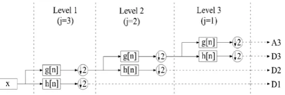
the so-called discrete wavelet transform (DWT). Notably, the DWT can be efficiently computed by means of a digital filter bank comprising a sufficient number of the (same) “building block” repeated in series as shown in Figure 1 in a multi-resolution analysis framework (Daubechies 1992, Vetterli and Herley 1992, Goswami and Chan 1999). Each building block corresponds to a particular scale or analysis “level” and consists of a high-pass filter with coefficients h[n]; n=1,2,…,N, a low-pass filter with coefficients g[n]; n=1,2,...,N, and a dyadic down-sampler (i.e., a mechanism of reducing the sampling rate by retaining every other sample of the input discrete-time signal) applied to the output of each of the previous filters. These filters are designed such that no energy is lost during transformation/processing of the input signal. At each level corresponding to the scale a=2-j the spectrum of the input discrete-time signal is split into two parts separating the high frequency components, represented by the “detail” sequence of wavelet coefficients DJ+1-j

upon down-sampling, from the low frequency components, represented by the “approximation” sequence of coefficients AJ+1-j upon down-sampling (see e.g. Vetterli and

Herley 1992). The full DWT requires J=log2R total number of levels to be considered and at each level the number of coefficients in the output sequences upon down-sampling is R/2(J

+1-j)_{. Therefore, the DWT is non-redundant: it produces exactly R coefficients given an R-long} discrete-time signal which preserve the signal energy E.

Figure 1: Typical dyadic discrete wavelet transform (DWT) analysis filter bank with J=3 scales for

In this respect, the processing of a given signal by a DWT filter bank begins by extracting, first, the highest frequency components at the lowest scale (i.e., for the largest j

value) and proceeds at each level by extracting lower and lower frequencies, that is, the values of j follow a descending order: j=J,J-1,…,1 (see also Figure 1). The detail (or wavelet) coefficients at each scale capture only the part Ej of the total signal energy defined as

[ ]

,

j j

k

E =

∑

where it is understood that summation is over all coefficients DJ+1-j at scale j. Then, the

total energy of the signal is retrieved by summing the energy over all J scales, that is,

[ ]

j j

j j k

E =

∑

∑∑

under the assumption that the energy of the approximation coefficient at the final analysis level is negligible. To this end, note that the ratio

,

j j

E p

E

= (8)

gives the fraction of the total signal energy, contained within a particular frequency band corresponding to the j scale of the DWT analysis filter bank. It, therefore, characterizes a discretized version of the Fourier transform-based function |X(ω)|2/E within this band. Notably, the width and location on the frequency axis of the frequency band corresponding to a scale j does not only depend on the value of j, but also on the FD attributes of the filter h[n] or, equivalently, on the FD attributes of the underlying analysis mother wavelet. In the following section, a structural damage sensitive index, introduced in Ren and Sun (2008), is briefly presented which relies on computing the ratio in (8) of acceleration response signals from dynamically excited linear structures. Further, in section 4, the FD attributes of DWT filter banks using different analysing mother wavelets are presented, while the influence of these attributes for vibration-based structural damage detection is numerically demonstrated in section 5.

3. The relative wavelet entropy for structural damage detection

SWE _jln( _j),

j

p p

= −

∑

where pj is the positive ratio in (8) with 0≤pj≤1 (i.e., pj qualifies as a probability

distribution) and the summation involves all scales considered in an energy preserving DWT filter bank to transform a given signal x(t). The SWE was proved to be an effective quantitative measure to characterize the information carried by signals at different scales (or corresponding frequencies) and time instants in certain biomedical applications (e.g., Blanco et al. 1998, Rosso et al. 2004). Interpreted from a structural dynamics viewpoint, the SWE of the acceleration response signal of a white noise excited lightly damped linear single degree of freedom structural system will attain a relatively small value compared to the SWE of the response signal of a white noise excited structure with multiple degrees of freedom. This is because the energy of the former signal will be well-localized in the FD around the natural frequency of the system and, ideally, will be captured by a single pj corresponding to the

scale containing this frequency. The value of this particular pj will be close to unity and,

therefore, its contribution to the sum in (9) will be almost zero as the term ln(pj) will be

almost zero, and so will be the contributions of the ratios from all other scales whose value will be close to zero. However, the energy of the response signal of a multi-degree of freedom structure will be spread around the various different natural frequencies of the structure. Consequently, there will be several non-zero contributions to the sum in (9) and the overall value of SWE will be large. Clearly, the SWE is maximized for a white noise signal implying a highly “disordered” process, while the SWE of a very narrowband signal (close to a pure sinusoid) will be almost zero implying an “ordered” process.

To this end, note that structural damage causes a shift to the natural frequencies of a structure and this should reflect in changes to the values of the scale-dependent energy ratios in (8) obtained from linear structural response acceleration signals commonly considered in VSHM. In this regard, Ren and Sun (2008) proposed the use of the relative wavelet entropy defined by

RWE _jln j ,

j j

p p

q

 

= _ _

 

∑

as a structural damage sensitive index. In the last equation, pj is the scale dependent

location of the damaged-state structure and qj is the scale dependent energy ratio in (8) from a

response acceleration signal measured at the same point of the healthy-state structure. For structures with negligible damage close to the measurement location, it is expected that pj≈qj

for all considered j scales and thus RWE attains a negligible value, corresponding to an ordered process. For damaged structures, it is expected that the two ratios will differ across some of the scales due to a shift to the natural frequencies of the system yielding a large RWE value, corresponding to a “disordered” process. Larger values of RWE are expected at measurements points close to the damage and, therefore, comparing the RWE values computed from an array of sensors may achieve damage localization (Ren and Sun 2008, Yun et al. 2011).

Note that the RWE index in (10) is independent of time aiming to detect stationary structural damage. Since the underlying information for the detection of such kind of damage is associated with signal energy distribution in the FD, it is intuitive to expect that the RWE is strongly dependent on the FD properties of the wavelet filter bank used to compute the energy ratios appearing in (10) and the quality of FD resolution. The FD properties of four different wavelet filter banks are discussed in the next section focusing on the frequency resolution and selectivity across different scales. The influence of using different wavelet filter banks to the effectiveness of the RWE as a damage detection index for stationary damage is numerically assessed in Section 5.

4. Frequency domain attributes of Daubechies, Haar, Meyer, and harmonic wavelet

analysis filter banks

4.1.Daubechies wavelet analysis filter banks

across all dyadic scales. Consequently, they achieve sharp localization of signal energy in TD and preserve the input signal energy.

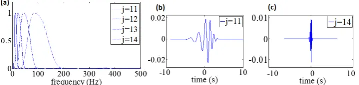
Nevertheless, the excellent TD localization capabilities of Daubechies wavelets, comes at the cost of relatively poor FD localization and discrimination across scales in typical Daubechies DWT filter banks. These issues are illustrated in Figure 2(a) which plots the FAS, |Ψ(ω/2j_{)|, of D20 Daubechies wavelets (defined using an N=20-long FIR filter reported}

in Daubechies 1992) for four adjacent scales. These FASs have been obtained by Fourier transforming D20 wavelets at different scales (Figures 2(b) and 2(c) plot two such wavelets). The wavelets are obtained by means of a standard algorithm which constructs recursively the so-called scaling function, φ(t), at first, and, then, the associated wavelet function at each considered scale j by relying on the following two-scale equations (see Goswami and Chan 1999)

1 1

(2 )j [ ] (2j ),

n

φ t ₌

∑

(11)

1 1

(2 )j [ ] (2j ).

n

ψ t ₌

∑

(12)

The sequence g1[n] in (11) are the N coefficients of the FIR filter defining the DN wavelets. Further, in (12), h1[n]=(–1)ng1[1–n]. Note that the signal analysis FIR filters appearing in Figure 1 for the DN wavelets are defined as g[n]=0.5⋅g1[–n] and h[n]=0.5⋅(–1)n

g1[n+1] (quadrature mirror construction).

Figure 2: Daubechies D20 wavelets for four different scales j from a filter bank with J=16 total

number of scales and Q= 0.46: (a) Normalized to the peak value FAS |Ψ(ω/2j)|, (b) wavelet in TD at scale j=11, and (c) wavelet in TD at scale j=14.

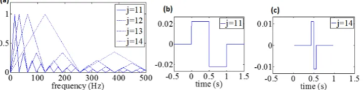
dominant lobe and several lower periodic sidelobs at higher frequencies. This is a consequence of the so-called uncertainty principle which holds for any Fourier pair: enhancing the energy localization of a function in the TD deteriorates its frequency resolution (i.e., widens its effective bandwidth) and vice versa (e.g., Cohen 1995). Note that the D20 wavelets shown in Figure 2 are rather smooth and their side lobs at higher frequencies are negligible. However, this is not the case for lower-order Daubechies wavelets. As a limiting case, Figure 3 provides similar plots as Figure 2 for the lowest possible order of Daubechies wavelets, D2, also known in the literature as “Haar” wavelets. The side lobs of the FASs of Haar wavelets are significant, while the frequency selectivity among scales in the lower frequencies is rather poor. Consequently, the use of such filter banks renders the task of assigning any single frequency band to the signal energy captured at a particular scale in (6),

Ej, a rather challenging task.

Figure 3: Daubechies D2 (or Haar) wavelets for four different scales j from a filter bank with J=16

total number of scales and Q= 0.49: (a) Normalized to the peak value FAS |Ψ(ω/2j)|, (b) wavelet in TD at scale j=11, and (c) wavelet in TD at scale j=14.

4.2.Meyer wavelet filter banks

Unlike the Daubechies wavelets which are compactly supported in the TD, the Meyer (mother) wavelet is compactly supported in the FD defined as (e.g. Daubechies 1992)

3 2 4

exp( / 2) sin 1 ;

2 2 3 3

3 4 8

Ψ( ) exp( / 2)cos 1 ;

2 2 3 3

0 ;

π π π

iω v ω ω

π

π π π

ω iω v ω ω

π otherwise    ₋  _{≤ ≤}  _ _ __   _{ }    =_{  } − _ ≤ ≤         (13)

[ ]

4 2 3

(35 84 70 20 ) ; 0,1

( ) .

0 ;

u u u u u

v u

otherwise

 − + − ∈

 = 

 (14)

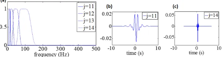
Orthogonal Meyer wavelet bases can be readily constructed and used to obtain energy preserving CWT in (3). In fact, Lee et al. (2014) considered the Meyer CWT to identify the potentially damaged connections in trusses by relying on the RWE from signals measured at healthy and damaged connections from a single excitation test. However, there exist DWT filter bank constructions comprising FIR filters (as in Figure 1) that approximate the Meyer-based CWT using a dyadic FD discretization scheme Misiti et al. (2000). Such a Meyer DWT filter bank is used in the numerical applications of section 5 since it is much more efficient to compute and therefore more likely to be adopted in computing wavelet coefficients on on-board micro-processors for wireless sensors used in VSHM (e.g., Lynch 2007, Yun et al. 2011).

Figure 4(a) plots the FAS of Meyer wavelets at four adjacent scales. Compared to the Daubechies wavelets of Figures 2(a) and 3(a), overlapping in the FD is observed only between neighbouring wavelet scales and there are no side lobs at high frequencies. Therefore, DWT filter banks of Meyer wavelets attain enhanced frequency selectivity among scales compared to Daubechies wavelets. However, as in the case of Daubechies wavelet filter banks, the frequency resolution deteriorates in higher frequencies as the wavelets becomes better localized in TD at lower scales (larger values of j). This issue is further discussed in the following sub-section.

Figure 4: Meyer wavelets for four different scales j from a filter bank with J=16 total number of

scales and Q= 0.68: (a) Normalized to the peak value FAS |Ψ(ω/2j)|, (b) wavelet in TD at scale j=11, and (c) wavelet in TD at scale j=14.

4.3.Constant Q-analysis wavelet filter banks

The ability of the square magnitude of the CWT and of the DWT (i.e., of the |C(α,b)|2 and of the |Cj[k]|2, respectively) to resolve the frequency components of any signal in time relies

scaling parameter a takes on smaller values (or as j assumes higher values in the case of DWT) the wavelets are compressed in the TD. However, the number of the wavelet zero-crossings (i.e., oscillations) remain the same and, thus, the wavelet FAS becomes wider, due to the uncertainty principle, while it shifts towards higher frequencies since the effective frequency in (4) increases. The above points can be readily observed in Figures 2 and 3: the width of the main lobe of the wavelet FΑS widens as the average frequency content, characterized by the central or the peak frequency of the main lobe, increases. This well-known property of the standard CWT in (5) is called constant-Q analysis, where Q is defined as the ratio of the effective frequency over the effective bandwidth at each analysis level or scale (see also Brown 1991). Consequently, the dyadic DWT filter banks assume a constant Q across scales or analysis levels (note that the value of Q is reported for the filter banks of Figures 2 to 4).

In many signal analysis applications a constant Q-analysis is favourable. This is because high-frequency components in time-series are usually well-localized in time, while low-frequency trends are well-spread in time. Nevertheless, this is not necessarily true in processing acceleration response signals from dynamically excited linear structures whose location of the dominant frequency components on the FD depends on the structural natural frequencies. The natural frequencies of lightly damped linear structures are well-localized in the FD and may lie anywhere on the frequency axis. In this regard, the use of non-constant Q wavelet analysis filter banks is a reasonable consideration in order to target natural frequencies related to higher modes of vibration effectively. The wavelet family presented in the next subsection can readily achieve custom-made non-constant Q wavelet analysis filter banks. These considerations have important practical implications to the effectiveness of the RWEin (10) for structural damage localization purposes as will be numerically illustrated in section 5.

4.4.Harmonic wavelet filter banks

( )

₍

_{[ ]}

_{[ ]}

₎

₍

_{[ ]}

_{[ ]}

₎

[ ]

[ ]

( )

0 ; .

o o

j k

o o

j k

T i kT

p j m j p j m j

m j p j

T T

otherwise ω ω

π

π _ω π

ω

 ₋ 

Ψ = _ _

− _ − _

≤ ≤

Ψ =

(15)

where Το is the total length (duration) of the time interval considered in the analysis. In the last equation, the sequences (vectors) p and m contain integer positive numbers. It was shown in Newland (1994), that a collection of harmonic wavelets spanning adjacent non-overlapping intervals at different scales on the FD forms a complete orthogonal basis. This can be achieved by proper definition of the p and m sequences. Then, the HWT, computed by substituting the inverse Fourier transform of (15) in (5), produces coefficients Cj[k] which

preserve the input signal energy.

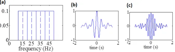
Importantly, note that at scale j the effective bandwidth of the HWT is (p[j]-m[j])2π/Το

Figure 5: Harmonic wavelets 10Hz constant bandwidth filter bank: (a) FAS for 4 different scales with

central frequencies denoted by broken lines, (b) real part harmonic wavelet with 15Hz central frequency, (c) real part harmonic wavelet with 35Hz central frequency.

Nevertheless, the aforementioned “freedom of choice” of HWT comes at the cost of relatively poor time localization as evidenced by comparing the wavelets plotted in TD in Figure 5 compared to those in Figures 2 to 4. In fact, harmonic wavelets can be viewed as the complex counterpart of the so-called “Shannon wavelets” associated with the Littlewood-Paley basis (see for example Daubechies 1992 and Vetterli and Herley 1992), which are well-known for their poor time localization properties. Still, for stationary damage detection, poor time-localization attributes is of secondary importance. From a computational viewpoint, robust fast Fourier transform (FFT)-based algorithms have been proposed by Newland (1994) and Newland (1999) for the efficient computation of non-redundant as well as for redundant HWT on the FD. A custom-made implementation of Newland’s FFT-based algorithm is used to compute non-constant Q HWT considered in section 5.

5. Numerical Assessment of different wavelet families for relative wavelet

entropy-based damage detection

5.1.Benchmark Structural Models

For the purposes of this study, finite element (FE) models corresponding to a healthy and a damaged state of two different structures, namely, an aluminum space truss and a simply supported steel beam, are considered. Note that lab specimens of similar structures have been adopted by Ren and Sun (2008), i.e., a simply supported beam, and by Yun et al. (2011), i.e., a space truss, to attest the applicability of the RWEfor damage detection from linear response acceleration signals obtained by tethered and by wireless sensors, respectively.

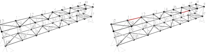
members and each bay is a cube with 707mm long side. The members shown in dark grey in Figure 6 have 22mm diameter and 1mm wall thickness, while the members shown in light grey are 30mm in diameter and 1.5mm wall thickness. The truss is modelled in SAP2000 FE commercial software using standard linear one-dimensional elements. Gravitational masses of 0.44kg are lumped at each of the 36 nodes of the FE model. Additional gravitational masses of 1.75kg are assigned to nodes 1,7,30, and 34, and of 2.75kg are assigned to nodes 20, 26, and 32. These additional masses ensure that the first six natural frequencies corresponding to predominantly bending mode shapes along the vertical plane of the truss are “clustered” together in pairs as reported in Table 1 below (see also Humar et al. 2006). A damaged state of the truss structure is further modelled by reducing the axial rigidity of the two truss members shown in red in the right panel of Figure 6 by 50%.

Figure 6: Space truss FE models: healthy state (left panel) and damaged state (right panel).

Furthermore, a 5m long steel IPE300-profiled beam resting on simple supports at both ends is also modelled using the standard FE method. The beam has cross-sectional area of 53.8cm2 and in-plane moment of inertia along its “strong axis” of 8360cm4. It is modelled in SAP2000 FE software using the grid of 4-node shell elements with 6 degrees-of-freedom (DOF) per node shown in Figure 7. The material mass density is taken equal to 7849kg/m3 and the elastic modulus is equal to 210GPa. A damaged state of the above beam is further modelled by reducing the cross-sectional area by 50% at the mid-span and at the quarter spans as shown in Figure 7.

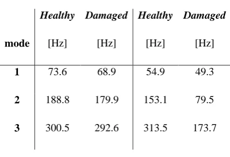
Table 1 lists the natural frequencies corresponding to the first three vertical (gravitational) in-plane modes of vibration of the considered FE models obtained by means of standard modal analysis. In all the ensuing dynamic analyses a critical damping ratio of 1% for all vibration modes is assumed.

Table 1: Natural frequencies corresponding to in-plane vertical bending mode shapes for the FE

models shown in Figures 6 and 7.

Space Truss Model Steel Beam Model

Healthy Damaged Healthy Damaged

mode [Hz] [Hz] [Hz] [Hz]

1 73.6 68.9 54.9 49.3

2 188.8 179.9 153.1 79.5

3 300.5 292.6 313.5 173.7

5.2.Excitation forcing functions and response acceleration signals

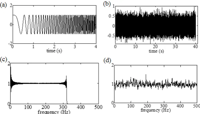
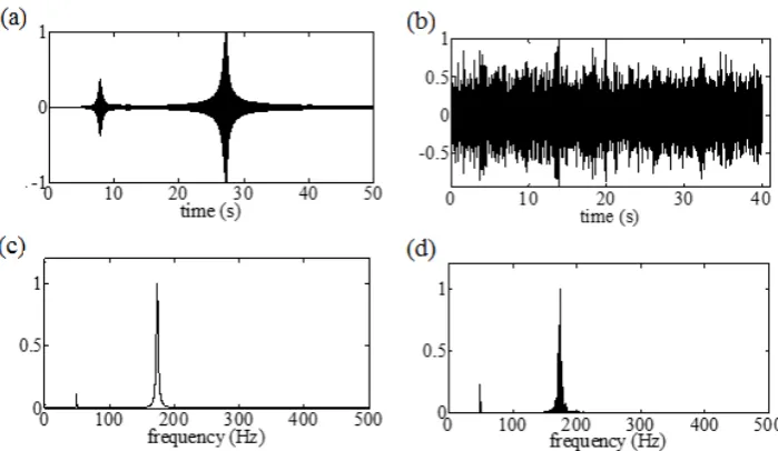
Figure 8: Sine-sweep (only first 4s shown) and white noise forcing functions in the time domain, (a)

and (b), and in the frequency domain, (c) and (d), respectively.

Standard linear response history analyses are undertaken in SAP2000 FE software to obtain response acceleration signals of the FE models in Figures 6 and 7 exposed to the excitations of Figure 8. For the case of the space truss FE models, the forcing functions are applied to node 5 along the gravitational axis (see Figure 6). For each individual forcing function, the vertical response acceleration time traces are obtained at 9 equidistant measurement points coinciding with the nodes 1 to 9 of the FE model in Figure 6. For the case of the beam models, the forcing functions are applied as point loads along the vertical axis at mid-span in the middle of the upper flange. For each individual forcing function, the vertical response acceleration traces are obtained at 15 measurement nodes along the length of the beam located on the upper flange (nodes 1 to 15 indicated in Figure 7).

To illustrate point (I), the acceleration response signals at the quarter-span of the damaged beam model obtained for the SS and from the WN excitations are plotted in Figures 9(a) and 9(b), respectively. The corresponding FASs normalized to their peak value are shown in Figures 9(c) and 9(d): they are identical exhibiting two spikes at the first and the third natural frequency (the forcing function applied at mid-span cannot excite the second mode shape of the beam). However, the response signal of the WN excitation is stationary in time, while the response signal for SS excitation is non-stationary characterized by two prominent “bursts” in time. The first low-frequency burst corresponds to resonance of the SS input with the first natural frequency of the beam (left-most spike of the FAS), while the second burst has higher frequencies due to resonance of the SS excitation with the third natural frequency of the beam (right-most spike of the FAS). The reason for considering both sets of response signals (stationary and non-stationary) is to test whether the above differences in the TD might influence the potential of the RWE for damage detection depending on the wavelet filter bank used, given that the time localization capabilities of certain wavelet families considered (in particular of the harmonic wavelets in Figure 5) are poor.

Figure 9: Response acceleration signals recorded at node 3 of the damaged beam in Figure 7 under

sine-sweep and white noise excitation in the time (a) and (b), and in the frequency domain (c) and (d), respectively.

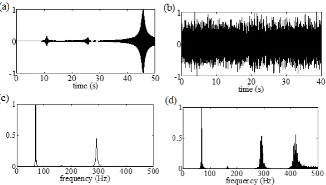
mode shapes with natural frequencies lying, purposely, outside the bandwidth of the SS excitation. The influence of this additional broadband high frequency content to the interpretation of RWE values computed using different wavelet filter banks is examined and discussed in subsequent sections.

Figure 10: Response acceleration signals recorded at node 4 of the damaged space truss in Figure 7

under sine-sweep and white noise excitation in the time (a) and (b), and in the frequency domain (c) and (d), respectively.

5.3.Wavelet analysis filter banks and scale-dependent relative wavelet entropy

filter banks is carried out using the built-in functions of the MATLAB-based wavelet toolbox developed by Misiti et al. (2000).

Table 2: Frequency domain attributes of the first 10 analysis levels for the considered wavelet filter

banks

Analysis

Level

(scale)

D20 Daubechies

wavelet filter bank

(Q≈0.46)

D2 Daubechies or

Haar wavelet filter

bank (Q≈0.49)

Meyer wavelet filter

bank (Q≈0.68)

Effective range (Hz)* Effective Frequency (Hz)* Effective range (Hz)* Effective Frequency (Hz)* Effective range (Hz) Effective Frequency (Hz)

1 (j=16)

70.62-812.14 342.11 0-1024 498.05

179.2-674.13 331.68

2 (j=15)

45.85-412.66 171.05 0-558 249.03

85.33-341.33 165.84

3 (j=14)

21.48-207.66 85.53 0-267 124.51

42.67-170.67 82.92

4 (j=13)

10.41-100.66 42.76 0-130 62.26 22.4-85.33 41.46

5 (j=12) 5.13-51.29 21.38 0-64 31.13 11.2-42.67 20.73

6 (j=11) 2.55-25.45 10.69 0-32 15.56 5.33-21.33 10.37

7 (j=10) 1.27-12.68 5.35 0-16 7.78 2.8-10.67 5.18

8 (j=9) 0.63-6.33 2.67 0-8 3.89 1.4-5.33 2.59

9 (j=8) 0.32-3.16 1.34 0-4 1.95 0.67-2.67 1.30

10 (j=7) 0.16-1.63 0.67 0-2 0.97 0.35-1.32 0.65

*Values accounting for only the main lobe of the FAS of the scaled wavelets

analysis is carried out by means of a custom-made code implementing the FFT-based algorithm described by Newland (1994 and 1999).

Next, the relative wavelet energy in (6) is computed from the wavelet coefficients of the response acceleration signals (healthy and damaged states) at each scale of the 4 different wavelet filter banks. Subsequently, the following “scale-dependent” contributor to the overall RWEin (10) is calculated for all measurement points of the damaged models

( )

RWE _jln j

j

p

j p

q

 

= _ _

 .

(15)

In the last equation, qj is the relative wavelet energy at scale j computed from the

simulated response signals of the “healthy” FE models, while pj is the relative wavelet energy

at scale j corresponding to response signals of the damaged state. The consideration of the above scale-dependent RWE(j) makes possible to discriminate the contributions to the overall in (10) from each wavelet analysis level. Therefore, it serves well the purpose of assessing the influence of the FD attributes of the different wavelet filter banks considered (i.e., frequency selectivity among scales and Q value) to the computed values of the RWE index. Finally, it is noted that no hard-thresholding is applied to the RWE as has been proposed by Ren and Sun (2008) to sharpen damage localization by keeping only the values of the RWE above a certain threshold. This is because this study focuses on gauging the influence of using different wavelet filter banks to the computation of the RWE across different scales, rather than the potential of RWE for damage localization. The latter issue is well-established in the literature (Ren and Sun 2008, Yun et al. 2011, Lee et al. 2014). Therefore, the next sub-section presents and discusses “raw” scale-dependent RWE(j) data obtained from the various analyses undertaken without any further filtering or processing.

5.4.Numerical results and discussion

value of the RWE(j) at a particular frequency and measurement point indicates a potential local damage at the considered point captured by a change to the response signal energy between the damaged state and the healthy state structure carried by the damaged state signal

at the considered frequency. Therefore, large values of the RWE(j) are expected at scales containing the natural frequencies of the damaged state reported in Table 1. Moreover, in all bar-charts of Figures 11-17 an additional row along the spatial axis located at the origin of the frequency axis and denoted by the symbol Σ is incorporated, which plots the RWE in (10), that is, the sum of the scale dependent RWE(j) across all scales as considered by Ren and Sun (2008).

By examining, first, the set of RWEplots in Figures 11(a)- 14(a) (space truss excited by the non-stationary SS force bandlimited to 320Hz of Figure 8(a)), it is noted that acceptable damage localization is achieved for all four filter banks considered in this study indicated by large RWE values at the 3rd and 7th measurement points. In the case of the smooth Daubechies D20 wavelets and of the Meyer wavelets, the RWE values are contributed from a single scale (j=13) or analysis level 4, with effective ranges that contain the first damaged natural frequency of the space truss (at 68.9Hz), as shown in Table 2. However, in the case of the Haar wavelet basis, certain non-zero RWE values are also contributed from the j=15 scale (at only three measurement points), centred at a frequency close to the third damaged natural frequency at 292.6Hz. The D20 and Meyer wavelets cannot capture this change since the central frequency at j=15 is much lower from the third damaged natural frequency, while at the highest scale (j=16) the corresponding frequency band spanned is so wide that no changes to the information carried by the response signals associated with the third mode shape can be resolved. Notably, this is not the case with the harmonic wavelets which resolve consistently, at all measurement points, changes to both the first and the third natural frequencies due to damage. Therefore, the non-constant Q harmonic wavelet filter bank with, theoretically, zero overlapping among scales offers a more robust RWE-based damage detection compared to the other DWT filter banks as it draws information about the damage from both the excited mode shapes at all measurement points.

reflected on the higher Q value. In particular, note that at j=15 scale both the above filter banks have almost the same “central” or effective frequency and, therefore, the bandwidth spanned by the Meyer wavelet at that scale is approximately 50% smaller than the D20 filter bank, i.e., almost equal to the ratio of their Q values (0.68/0.46). Moreover, it is observed that non-zero RWE values are contributed by two different scales j=13 and 14 for the Meyer and the D20 filter banks. Since only a single natural frequency exists within the frequency bands spanned by these two scales, it is concluded that this is due to wavelet energy (spectral) leakage caused by the significant overlapping of the frequency bands of the above adjacent scales. More importantly, it is seen that the Haar wavelet filter bank fails to produce results amenable to a physically meaningful interpretation (Figure 12(b)). The non-zero RWE values are contributed from scales having very low effective natural frequencies. This phenomenon can only be attributed to the existence of significant side lobs of the FAS of Haar wavelets across scales in conjunction with the existence of broadband high frequency content in the considered set of response acceleration signals (compare the plots in Figure 3(a) and Figure 8(d)). As in the case of response signals from the SS excitation, the harmonic wavelet filter bank is able to resolve accurately the shifts of natural frequencies as they reflect to changes to the wavelet energy distribution captured by the RWE. Clearly, the fact that the two sets of response acceleration signals examined (i.e., due to the SS and WN excitations) have very different time-domain properties does not affect the ability of harmonic wavelets to represent correctly the frequency content even for the highly non-stationary signals despite their relatively poor time localization capabilities.

(a) (b)

(a) (b)

Figure 12: Scale-dependent RWE(j) in (16) and RWE in (10) (denoted by Σ) using the Daubechies D2

(or Haar) wavelet filter bank of Table 2 for the space truss of Figure 6 subject to (a) the sine-sweep and (b) the white noise excitation in Figure 8.

(a) (b)

Figure 13: Scale-dependent RWE(j) in (16) and RWE in (10) (denoted by Σ) using the Meyer wavelet

filter bank of Table 2 for the space truss of Figure 6 subject to (a) the sine-sweep and (b) the white noise excitation in Figure 8.

(a) (b)

Turning the attention to the RWE plots for the case of the beam FE model (Figures 15-17) it is seen that the Haar wavelet basis yields reasonable RWE values, as in the case of the truss structure excited by the SS forcing function, which clearly identify the location of the damage in the middle of the beam and indicate that two more locations of potential damage exist closer to the supports of the beam. However, significant leakage of the scale-dependent RWE(j) across scales is observed due to the poor frequency selectivity of the Haar wavelet filter bank. In the case of the Meyer wavelet filter bank, no energy leakage across scales is observed, but damage is detected based on the changes of the wavelet energy associated with a single (the 3rd_{) mode shape which dominates the overall response as seen is Figure 9 (the} right-most spike in the reported FASs has a significant higher amplitude from the left-most). Lastly, the non-constant Q harmonic wavelet filter bank yields non-zero RWE(j) contributions associated with wavelet energy changes between the healthy and the damaged state for both the excited modes (1st and 3rd) with insignificant leakage.

(a) (b)

Figure 15: Scale-dependent RWE(j) in (16) and RWE in (10) (denoted by Σ) using the Daubechies D2

(or Haar) wavelet filter bank of Table 2 for the beam of Figure 7 subject to (a) the sine-sweep and (b) the white noise excitation in Figure 8.

(a) (b)

(a) (b)

Figure 17: Scale-dependent RWE(j) in (16) and RWE in (10) (denoted by Σ) using a 128-scale

harmonic wavelet filter bank (3.91Hz bandwidth per scale) for the beam of Figure 7 subject to (a) the sine-sweep and (b) the white noise excitation in Figure 8.

Overall, the above numerical results suggest that the adopted harmonic wavelet basis spanning non-overlapping frequency bands among scales and maintaining the same level of (high) resolution for the full range of frequencies of interest is always able to discriminate changes to the distribution of the signal energy between the damaged and the healthy states manifested by a shift of all the excited structural natural frequencies. This is achieved no matter whether the recorded signals are stationary or non-stationary in the TD and with negligible spectral leakage which renders the interpretation of the results a straightforward task. This is not always the case for the dyadic DWT bases which capture structural damage manifested by non-zero RWE(j) values only when a particular scale corresponds to a relatively narrow band of frequencies and has an effective/central frequency lying close to a structural natural frequency. Further, in cases of severe overlapping of frequency bands among scales significant spectral leakage across scales is seen, which does not facilitate the interpretation of the results.

As a final remark, it is emphasized that the herein considered harmonic wavelet basis is not necessarily a recommended and, by no means, an optimal approach for wavelet transforming response acceleration signals for RWE-based damage detection. It has only been used in this study as an “extreme case” of a basis with good FD attributes vis-à-vis the

standard dyadic DWT filter banks considered in the literature. Apart from the HWT

response signals associated with structural damage (e.g., Yen and Lin 2000, Sun and Chang 2004). After all, the HWT can be loosely interpreted as a WPT of a Littlewood-Paley wavelet basis (Vetterli and Herley 1992). Still, a harmonic wavelet basis with constant frequency resolution across scales may be used as a reasonable approach for RWE-based damage detection where the natural frequencies of the (damaged) structure are not a priori known. In this case, a HWT with coarser resolution than what has been employed in this study (i.e., a reduced number of scales or wider bandwidth/scale) should be considered to keep the computational cost low for practical implementation, especially in the case of decentralized VSHM using wireless sensors (Yun et al. 2011). In cases some prior knowledge about the natural frequencies of a given structure is available, a customized WPT (e.g., Yen and Lin 2000, Sun and Chang 2004) or a HWT spanning frequency bins of non-constant width (e.g., Giaralis and Spanos 2009) can be employed to achieve enhanced frequency resolution in the vicinity of the known natural frequencies and, therefore, to yield more efficient RWE-based damage detection.

6. Concluding remarks

A comprehensive numerical study was undertaken to assess the influence of the frequency domain (FD) attributes of wavelet analysis filter banks for structural damage detection and localization relying on the concept of the relative wavelet entropy (RWE): a well-established in the literature damage-sensitive index derived by wavelet transforming linear response acceleration signals from a healthy/reference and a damaged state of a given structure subject to broadband excitations. This work was motivated by a lack of comparative studies and practical recommendations for the computation of the RWE and by the observation that stationary (i.e., non-evolving in time) damage is detected by changes to the energy distribution of response acceleration signals from the healthy and the damaged state across the wavelet scales (or, equivalently, along the frequency axis), associated with damage induced shift of the natural frequencies.

duration sample of Gaussian white noise process. Four energy-preserving wavelet analysis filter banks with different FD attributes were employed to wavelet transform the response acceleration signals via algorithms which can be efficiently run on wireless sensors used for decentralized vibration-based structural health monitoring. RWE values for all sets of signals processed by the different wavelet filter banks were reported vis-à-vis. Focus was given on the scale-dependent contributors to the total RWE values to examine the ability of the different wavelet filter banks to resolve changes to the response signals’ energy distribution on the FD indicative of structural damage.

It is envisioned that the herein drawn qualitative remarks and practical recommendations on the efficiency of different energy-preserving wavelet bases to resolve structural damage will not only facilitate the use of the RWE for damage detection, but will also be useful for vibration-based structural health monitoring using compressive sensing data acquisition techniques (Baraniuk 2007). These techniques can derive the significant wavelet coefficients of signals in a single data acquisition step, provided that a wavelet basis with reduced spectral leakage across scales is utilized. Therefore, they may significantly reduce the computational cost and power consumption in wireless sensors for VSHM. Such considerations fall well beyond the scope of this paper and will be addressed by the authors in subsequent works.

Acknowledgements

This work has been funded by EPSRC in UK, under grant No EP/K023047/1. The first author acknowledges the support of City University London through a PhD studentship.

References

Baraniuk, R.G. (2007) ‘Compressive sensing’, IEEE Signal Processing Magnitude Vol.24, pp.118-121.

Blanco, S., Figliola, F., Quian Quiroga, R., Rosso, O.A. and Serrano, E. (1998) ‘Time– frequency analysis of electroencephalogram series (III): information transfer function and wavelets packets’, Physical Review E, Vol.57, pp.932-940.

Brown, J. C. (1991) ‘Calculation of a constant Q spectral transform’, Journal of the Acoustical Society of America, Vol. 89, No.1, pp.425–434.

Cohen, L. (1995) Time- Frequency Analysis, New Jersey, Prentice-Hall.

CSI Analysis Reference Manual, for SAP2000, ETABS and SAFE (2007), Computers and

Structures Inc.

Daubechies, I. (1992) Ten Lectures on Wavelets, Philadelphia, SIAM.

Doebling, S.W., Farrar, C.R., and Prime, M. B. (1998) ‘A summary review of vibration-based damage identification methods’, Shock Vib. Dig., Vol. 30, No.2, pp.91–105.

Ewins, D. J. (2000) Modal Testing: Theory practice and application,2nd ed., Research Study Press, Baldock.

Giaralis, A. and Spanos, P.D. (2009) ‘Wavelet-based response spectrum compatible synthesis of accelerograms-Eurocode application (EC8)’, Soil Dynamics Earthquake Engineering,

Goswami, J.C. and Chan, A.K. (1999) Fundamentals of wavelets: Theory, algorithms, and applications, New York, Wiley.

Humar, J., Bagchi, A. and Xu, H. (2006) ‘Performance of vibration-based techniques for the identification of structural damage’, Structural Health Monitoring, Vol. 5, No. 3, pp.215-241.

Lee, S.G., Yun, G.J. and Shang, S. (2014) ‘Reference-free damage detection for truss bridge structures by continuous relative wavelet entropy method’, Structural Health Monitoring,

Vol. 13, No. 3, pp.307-320.

Lynch, J.P. (2007) ‘An overview of wireless structural health monitoring for civil structures’,

Proceedings of the Royal Society, London A, Vol. 365, pp. 345-372.

Misiti, M., Misiti, Y., Oppenheim, G. and Poggi, J. (2000) Wavelet Toolbox, The MathWorks Inc.

Newland, D. E. (1994) ‘Harmonic and musical wavelets’, Proceedings of the Royal Society,

London A, Vol. 444, pp.605-620.

Newland, D.E. (1999) ‘Ridge and phase identification in the frequency analysis of transient signals by harmonic wavelets’, Journal of Vibrations and Acoustics, Vol. 121, No. 2, pp.149-155.

Ren, W.-X. and Sun, Z.-S. (2008) ‘Structural damage identification by using wavelet entropy’, Engineering Structures, Vol. 30, No.10, pp. 2840-2849.

Reynders, E. (2012) ‘System identification methods for (operational) modal analysis: review and comparison’, Arch. Comput. Methods Eng., Vol. 19, No.1, pp.51-124.

Rosso, O.A., Martin, M.T., Figliola, A., Keller K. and Plastino, A. (2006) ‘EEG analysis using wavelet-based information tools’, Journal of Neuroscience Methods, Vol. 153, No. 2, pp.163-182.

Spanos, P.D., Giaralis, A., Politis, N.P. and Roessett, J.M. (2007) ‘Numerical treatment of seismic accelerograms and of inelastic seismic structural responses using harmonic wavelets’, Computer-Aided Civil and Infrastructure Engineering, Vol.22, No. 4, pp.254-264.

Sun, Z. and Chang, C.C. (2004) ‘Statistical wavelet-based method for structural health monitoring’, Journal of Structural Engineering, Vol. 130, No. 7, pp.1055-1062.

Vetterli M. and Herley, C. (1992) ‘Wavelets and filter banks: theory and design’, IEEE Transactions of Signal Processing, Vol. 40, No. 9, pp.2207-2232.

Yen, G.G. and Lin, K.-C. (2000) ‘Wavelet packet feature extraction for vibration monitoring’, IEEE Transactions on Industrial Electronics, Vol. 47, No. 3, pp.650-667.