Review and application of Rainflow residue processing techniques for accurate fatigue damage estimation

Review and application of Rainflow residue processing techniques

for accurate fatigue damage estimation

Gabriel Marsh

a,b,⇑

_{, Colin Wignall}

b

_{, Philipp R. Thies}

a,c

_{, Nigel Barltrop}

a,d

_{, Atilla Incecik}

a,d

_,

Vengatesan Venugopal

a,e

, Lars Johanning

a,c

a

Industrial Doctoral Centre for Offshore Renewable Energy, The University of Edinburgh, King’s Buildings, Edinburgh EH9 3JL, UK b_{E.ON Technologies Limited, Technology Centre, Ratcliffe on Soar, Nottingham NG11 0EE, UK}

c

College of Engineering, Mathematics and Physical Science, Renewable Energy Research Group, University of Exeter, Penryn Campus, Penryn TR10 9EZ, UK d

Department of Naval Architecture, Ocean and Marine Engineering, University of Strathclyde, Glasgow G4 0LZ, UK e

Institute for Energy Systems, School of Engineering, The University of Edinburgh, King’s Buildings, Edinburgh EH9 3JL, UK

a r t i c l e i n f o

Article history:

Received 30 June 2015

Received in revised form 28 September 2015 Accepted 6 October 2015

Available online 20 October 2015

Keywords:

Cyclic counting methods Load histories Rainflow residue Random loading Variable amplitude fatigue

a b s t r a c t

Most fatigue loaded structural components are subjected to variable amplitude loads which must be processed into a form that is compatible with design life calculations. Rainflow counting allows individual stress cycles to be identified where they form a closed stress–strain hysteresis loop within a random signal, but inevitably leaves a residue of open data points which must be post-processed. Comparison is made between conventional methods of processing the residue data points, which may be non-conservative, and a more versatile method, presented by Amzallag et al. (1994), which allows transition cycles to be processed accurately.

This paper presents an analytical proof of the method presented by Amzallag et al. The impact of residue processing on fatigue calculations is demonstrated through the application and comparison of the different techniques in two case studies using long term, high resolution data sets. The most significance is found when the load process results in a slowly varying mean stress which is not fully accounted for by traditional Rainflow counting methods.

Ó2015 The Authors. Published by Elsevier Ltd. This is an open access article under the CC BY license (http://creativecommons.org/licenses/by/4.0/).

1. Introduction

The calculation of conservative load cycle spectra is a funda-mental aspect of fatigue design, requiring an estimate to be made of expected operational loading conditions. Complex lifecycle load-ing may be simplified by dividload-ing the process into discrete load cases, such as take-off and steady flight conditions for the analysis of aircraft components. Fatigue life can then be quantified in terms of time to crack initiation through the concept of linear damage accumulation, or by the application of crack growth models. Both approaches utilise information about the range, mean and number of stress cycles that will occur[1].

The identification of individual fatigue loading cycles within a random stress amplitude time series is achieved through the use of a suitable cycle counting algorithm. Typical methods include level-crossing counting, range-pair counting, reservoir counting, and Rainflow counting. Variations of these algorithms are included in the ASTM cycle counting standard[2].

1.1. Background to the Rainflow counting algorithm

Rainflow (RF) counting has become the most widely accepted method for the processing of random signals for fatigue analysis, and testing has demonstrated good agreement with measured fati-gue lives when compared to other counting algorithms [3]. The concept was first developed by Matsuishi and Endo [4], where the identification of cycles was likened to the path taken by rain running down a pagoda roof. In the paper, the authors defined a full RF cycle as a stress range formed by two points which are bounded within adjacent points of higher and lower magnitude; as the stress path returns past the first turning point it can be seen to form a cycle as described by a closed stress–strain hysteresis loop (Fig. 1a). For the case where successive stress points are either converging or diverging, the hysteresis curves do not form a closed loop (Fig. 1b). For this case the authors assumed that fatigue damage could be attributed to each successive range as half-cycles. The method was further developed by Okamura et al.[5]and Downing and Socie[6]as a vector based algorithm which identi-fied full RF cycles and half-cycles based on a three-point criteria without the need to rearrange the data series, and enabled efficient utilisation in computer software. This greatly reduced the data

http://dx.doi.org/10.1016/j.ijfatigue.2015.10.007

0142-1123/Ó2015 The Authors. Published by Elsevier Ltd.

This is an open access article under the CC BY license (http://creativecommons.org/licenses/by/4.0/).

⇑ Corresponding author at: E.ON Technologies (Ratcliffe) Limited, Technology Centre, Ratcliffe on Soar, Nottingham NG11 0EE, UK.

E-mail address:[email protected](G. Marsh).

Contents lists available atScienceDirect

International Journal of Fatigue

storage requirements as the stress signal could be read into the algorithm in real-time and processed directly into RF cycle spectra. This definition of the algorithm has been refined and included in the ASTM cycle counting standard [2]. Amzallag et al. [7] conducted a wide ranging industry consultation and defined a standardised algorithm which identified RF cycles based on a four-point criterion. The three and four point versions of the algorithm were shown to identify the same cycles by McInnes and Meehan[8], who presented a series of fundamental properties of RF counting to demonstrate the equivalence of the two methods. Although various forms of the RF algorithm exist, the four-point algorithm presents the most unambiguous criterion for the identification of closed hysteresis loops, and is defined below.

1.2. Four-point Rainflow counting criterion

RF counting requires the time history to be first processed into a Peak-Valley (PV) series consisting of local maxima and minima which define the turning points, or load reversals, of a time series. Pointxmis identified as a local maxima or minima within a time

series of lengthMif,

xm1<xm>xmþ1orxm1>xm<xmþ1 m¼2;3;4;...;M1 ð1Þ

Once the data have been filtered according to the PV criteria, full RF cycles are identified in the range formed by points xnto

xn+1if they meet the four-point criterion,

jxn1xnj P jxnxnþ1j 6 jxnþ1xnþ2j n¼2;3;4;. . .;N2

ð2Þ

whereNsignifies the length of the PV filtered series. If the range formed by points xn to xn+1 meets the four-point criterion then

the points are recorded before deleting them from the PV series, thus enabling further ranges to be formed between the adjacent pointsxn1andxn+2. The process is repeated until all ranges which

meet the four-point criterion are recorded and deleted from the PV series.

Storage of the counted ranges is achieved with a two dimensional histogram to record the cycle stresses. The form of the histogram may be chosen to preserve detailed cycle hysteresis information which may be significant in further statistical analysis,

for example with the min–max or max–min matrices where cycles are binned according to the loading sequence[9]. As a minimum, the histogram should record the cycle range and mean stress levels as inputs to final damage calculations.

1.3. Rainflow residue

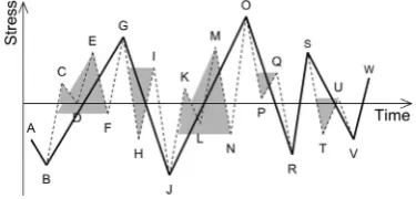
Once all full RF cycles which meet the four-point criterion have been identified and deleted from the PV series, a ‘residue’ of data points will typically remain. The residue consists of a series of diverging data points from the start to the maximum and mini-mum points, followed by a converging section of points to the end of the PV data series. Referring toFig. 2, no remaining closed hysteresis cycles can be identified within a diverging or converging series as no further ranges are bounded by adjacent points of higher and lower value. However, as the stress path formed by the residue constitutes some of the largest ranges in the original series, they should be accounted for if a conservative estimate of fatigue damage is to be made. Two dominant methods exist in the literature to process the RF residue and are outlined in Sections 2.1 and 2.2.

Whenever a subset of a longer time history is RF counted, cycle ranges which are formed between points which span beyond the subset have the potential to be cropped. If there is a large variation in the mean stress level, which is not fully contained within the subset period, then some of the largest cycles will not be accounted for. These cycles are termed ‘‘transition cycles” or ‘‘ground cycles” [10], and a degree of artificiality will be introduced if the residue data points are processed as an isolated set, as closed hysteresis cycles cannot be formed. The only way to accurately identify all RF cycles within a data set according to the four-point criterion is to process the entire time history consecutively, yet the applica-tion of RF counting algorithms must always utilise a finite length of data, as chosen by the analyst and by limitations on computational capacity.

Glinka and Kam [11] presented an approach which allowed

extended time periods to be read and processed incrementally, thus limiting the required computational capacity by minimising the amount of data required to be handled by the RF algorithm at any one time. A more versatile method is included in Amzallag et al.[7, pp. 292–293]which addresses the same issue by concate-nating consecutive residue periods which remain after RF process-ing. However, although the method allows transition cycles to be accounted for accurately according the four-point criterion, it has not found widespread acknowledgement and no generalised proof of the methodology has been presented.

[image:2.595.64.253.66.283.2]

The three methods of processing the RF residue periods are presented in Section2below. An analytical proof is presented in Section 3 which demonstrates the equivalence of cycles which are identified from the residue concatenation methodology out-lined in[7]with those which would be identified by RF processing a continuous series. In Section 4, the different approaches are Fig. 1.(a) Stress time series of turning points and the corresponding closed stress–

strain hysteresis loop formed by pointsn,n+ 1 andn0_{. (b) Diverging stress time}

series and the corresponding open stress–strain hysteresis curves.

Fig. 2.Residue remaining after application of the four-point criterion (points connected by solid line). Full RF cycles would be identified between pointsC–D,E–F,

[image:2.595.333.521.633.723.2]

applied to two case studies in order to illustrate the potential impact of the choice of residue processing method on calculated fatigue damage. Finally, Section5outlines the suitability of each of the three methods for practical applications.

2. RF residue processing methodologies

The three distinct methods available for processing the residue data points are described below and presented in the process diagram inFig. 3.

2.1. Half-cycle counting methodology

This approach is identified in the original definition of RF count-ing given by Matsuishi and Endo[4], where the authors assumed that each successive range will attribute half a cycle of fatigue damage in the material. FromFig. 2, subsequent half-cycle ranges are identified between pointsA–B,B–G, G–J,J–O,O–R,R–S,S–V,

V–W. At least twice as many ranges will be identified from the residue data points as would be identified as fully closed cycles. Therefore, when the counted residue cycles are stored in the RF histogram the number of cycles added to each bin is reduced by a factor of 0.5. The ASTM RF counting definition of the three-point algorithm[2, pp. 5–6] is capable of identifying half-cycles which occur up to the maximum data point in the series; after completion of the algorithm, the residue data points following the maximum still remain and must be accounted for as half

cycles. Half-cycle counting may be applied directly to the residue which remains from application of the four-point RF criterion, and the resulting cycles can be shown to be identical to those produced by the three-point algorithm.

2.2. Simple Rainflow counting methodology

If the stress time history is representative of a repeated loading sequence then all residue data points will ultimately form fully closed cycles as they will fall between repeated extremes. With the four-point algorithm this can be achieved by joining two repeated residues and then reapplying the four-point criterion (Eq.(2)). Closed cycles can then be identified between the repeated maximums, leaving the residue points outside of the maximums which can then be discarded. This is expressed as [residue] + [residue]?[residue] + {cycles}[7].

FromFig. 2, the residue series is repeated to give a sequence

A–B–G–J–O–R–S–V–W–A–B–G–J–O–R–S–V–W. Eq. (1) is then reapplied and the repeated pointAmust be deleted to ensure that the PV sequence is maintained. Eq.(2)is then reapplied to identify closed cycles from all points that fall betweenJand repeated point

O; ranges are formed by pointsV–W,R–S,B–G,J–O. The remaining points account for the repeated residue, and are therefore discarded.

[image:3.595.150.460.374.729.2]

The simple RF counting methodology is implemented in the three-point algorithm by rearranging the stress time series to start and end with the maximum data point prior to PV processing and

Fig. 3.RF counting process diagram for long time periods (modified from[12]). Grey boxes identify steps which relate to the residue processing methods outlined in Sections

RF counting, and will identify identical cycles[8]. Therefore, the approaches implemented in [2, pp. 6–7], [6, p. 32], [7] and [8] are equivalent.

2.3. Residue concatenation methodology

The following steps apply the residue concatenation procedure outlined in[7, pp. 292–293]to the simple case of two PV periods, with reference toFigs. 4 and 5;

1. Define two series of PV processed data pointsA1,B1,C1,. . .,H1

andA2,B2,C2,. . .,H2.

2. Apply the four-point criterion (Eq.(2)) to both series to identify all full RF cycles. Full cycles are identified between pointsD1–E1,

andE2–F2(Fig. 4a).

3. Store the cycles and delete the identified data pointsD1,E1and

E2,F2from the respective PV series (Fig. 4b). No more full RF

cycles can be identified according to Eq. (2). The remaining points form the two RF residues.

4. Concatenate the two residues in their original chronological order. Apply the PV criteria to the concatenated pointsH1and

A2to ensure the PV series is maintained. Delete pointH1(Fig. 4c).

5. Repeatedly apply the four-point criterion to the concatenated series until all fully closed RF cycles have been stored and removed. (Fig. 5a–c). Full RF cycles are identified between pointsA2–B2,F1–G1,C2–D2sequentially.

6. The remaining residue points are shown inFig. 5d, and must be processed by either half-cycle or simple RF counting. In practice, successive residue periods may be concatenated to allow additional closed hysteresis cycles to be unlocked.

3. Equivalence of concatenated series

The residue concatenation method outlined in Section2.3can be shown to account accurately for transition cycles between con-secutive periods by following the fundamental properties of the four-point criterion presented by McInnes and Meehan[8].

3.1. Identical RF cycles are identified using residue concatenation as would be identified from a continuous series

[image:4.595.310.546.72.530.2]

McInnes and Meehan defined an ‘end-point bounded sequence’ (EPBS) as any series of data points in which the maximum and minimum values lie at the start and end of the series. As all points are bounded between these local extremes, all the ranges con-tained between the end points will form fully closed cycles accord-ing to the four-point criterion. The authors show that the full cycles contained within an EPBS are independent and unaffected by the Fig. 4.(a) Two separate PV series. (b) The residue series from which no further fully

closed RF cycles can be identified. (c) Concatenation of the two RF residue series in stress–time and stress–strain space.

[image:4.595.43.273.406.724.2]

data points which lie outside of the sequence (Property 3.5,[8, p. 552]). Furthermore, as the residue remaining from the four-point algorithm consists of a set of EPBSs from the PV series (Property 3.8,[8, p. 554]), all the ranges which meet the four-point criterion will do so independently of the data points which occur before or after the PV series. Therefore, according to these two properties, the specific RF cycles which can be identified from separate periods must also form valid cycles within a continuous series.

McInnes and Meehan also showed that the RF cycles which meet the four-point criterion will do so regardless of the order in which the criterion is applied (Property 3.3,[8, p. 551]). Therefore, the EPBSs which may be formed between residue periods when they are concatenated can release additional RF cycles which would otherwise have been identified from a continuous series.

Referring toFig. 4a, the data point subsetsC1,D1,E1,F1andD2,

[image:5.595.53.285.343.438.2] [image:5.595.145.459.497.738.2]

E2,F2,G2both form EPBSs and therefore, according to Property 3.5

[8, p. 552], the full cycles formed by the rangesD1toE1andE2toF2

are independent and unaffected by the concatenation of the two residues. PointsC1toG2then produce an EPBS within the

concate-nated residues which allows additional full cycles to be formed by the rangesA2–B2,F1–G1, andC2–D2(Fig. 5). According to Property

3.3[8, p. 551], the same cycles would be identified from a contin-uous series, although they would have been extracted in a different order.

3.2. Deleted residue end points do not affect the correct identification of RF cycles

RF cycles which fall within an EPBS that includes the end point in a residue series are not affected if the point must be deleted after concatenation in order to maintain the PV sequence. This is true because, although the first or last point in an EPBS might be deleted, the sequence would always be extended to a bounding point which is of greater range.Fig. 6demonstrates the three basic configurations for the connected ends of two concatenated resi-dues (additional permutations exist which are essentially mirror images in the horizontal and vertical planes).Fig. 6a shows the configuration where the PV sequence is maintained and no points are required to be deleted.Fig. 6b shows the case where one point must be deleted to fulfil the PV criteria and the EPBS formed byB1

toC1is extended toB1toA2as pointC1is removed.Fig. 6c shows

the case where both the concatenated end points must be deleted and the EPBSs formed byB1toC1andA2toB2are both extended to

the range formed byB1toB2. Therefore, Property 3.5[8, p. 552]

holds true when RF residues are concatenated and the PV criteria is reapplied.

4. Residue processing comparison using experimental data

The significance of the different residue processing methods can be compared by investigating their impact on calculated fatigue damage.

4.1. Fatigue damage comparison methods

The Palmgren-Miner linear damage hypothesis assumes that the fatigue damage in a loaded component can be expressed as the sum of damages contributed by each stress cycle,

D¼X

k

i¼1

ni

Ni ð

3Þ

whereDis fatigue damage fraction, andni/Niis the ratio of

opera-tional cycles to the maximum allowable number of cycles at each Fig. 6.Detail of the connected ends of two concatenated residues. Residue end

points are shown with a dot, deleted points (which do not meet the PV criteria) are indicated by a dotted line, and joined points are indicated by a dashed line.

stress range. Although fatigue crack propagation can be found to be influenced by the load sequence, the linear damage sum is com-monly used in cases which require a statistical representation of the loading, such as found with environmental loading where the load sequence is rarely well defined at the design stage. Therefore, the linear damage sum has been used for this analysis, although a more detailed fracture mechanics approach may also benefit from the ability to correctly identify large amplitude hysteresis cycles.

The maximum allowable number of cycles N is taken from

empiricalS–Ndata, as generalised by the Basquin relation,

logN¼logamlog

Dr

ð4Þ

whereD

r

is either stress range or amplitude (stress range will be used here in accordance with the RF cycle definition), m is the Wöhler exponent, and logais the intercept of the curve on the logN

axis. Combining Eqs.(3) and (4), the ratio of fatigue damages can be expressed as,

DA

DB¼

Pk

i¼1nAi

Dr

m i

Pk

i¼1nBi

Dr

m i

ð5Þ

where nA and nB are the cycle spectra produced by different RF

counting methods. It can be seen that, by taking the damage ratio, the loga intercept term cancels and the impact of the different counting methods is affected only by the Wöhler exponent from theS–Ncurve. It can also be seen that a hypothetical linear increase in stress ranges such as may arise from a stress concentration factor, for example, would also cancel with the damage ratio, indicating that the difference between the RF counting methods would be affected by the underlying load process, but not by the stress mag-nitude. As a fatigue endurance limit could be exceeded by such a linear increase in stresses any results calculated in this analysis would be trivial; i.e. the use of a constant gradientS–Ncurve means that the form of Eq.(5)enables the general case to be examined.

S–Ndata is typically derived from component testing with a zero mean cycle stress. However, stress cycles in the tensile range may produce greater levels of fatigue damage, andS–Ntest results are known to be strongly dependent on the mean stress level. Mean stress correction models may therefore be used to adjust the stress range prior to damage calculation fromS–Ncurves using,

Dr

r¼

Dr

0 1

r

r

UTS

Z!

ð6Þ

whereD

r

ris the stress range or amplitude at non-zero mean stress

r

,D

r

0 is the equivalent stress range or amplitude at zero mean

stress, and

r

UTS is the ultimate tensile strength of the material.

Values ofZ= 1 and Z= 2 give the Goodman and Gerber relations, respectively, while the Soderberg relation is given withZ= 1 and

r

UTSreplaced by the yield stress[1]. Mean stress correction models

are applicable in the tensile range only, thereforeD

r

r¼D

r

0is used

in compression.

The impacts of the residue processing methodologies were then assessed against the following variables;

The underlying load processes.

The Wöhler exponent used to calculate fatigue damage. The length of the subset period used for the half-cycle and

sim-ple RF methods outlined in Sections2.1 and 2.2.

4.2. Measured datasets

Two datasets representing different load processes were used to investigate the residue processing methodologies. The offshore measurement buoy shown inFig. 7a is governed by dynamic wave loading, but the mooring system is also effected by a semi-diurnal

tidal cycle. The offshore wind turbine shown inFig. 7b also experi-ences hydrodynamic loading, but the structural response is domi-nated by the aerodynamic and operational loads.

For the offshore measurement buoy, a load cell was used to measure forces located at the connection between the buoy and a catenary mooring line, recorded with a sample rate of 20 Hz. The force time series was then converted to stresses using the geometry of the attachment shackle. Details of the mooring system are outlined in[13].

For the offshore wind turbine support structure, strain gauge measurements were also recorded at 20 Hz sample rate and con-verted to time series stresses using the Elastic Modulus of the base material. The gauge was located away from any stress raising fea-tures at the base of the wind turbine near the mean water level, axially aligned with the cylindrical tower to measure the nominal bending stresses. Material constants for the measured components are shown inTable 1.

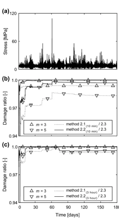
[image:6.595.324.525.336.703.2]

Fig. 8.(a) Stress time history from a catenary mooring attachment point. (b) Ratio of accumulated fatigue damages calculated using Eq.(5); damage produced by half-cycle and simple RF counting ten minute subsets, divided by the damage produced by RF counting the data continuously. (c) Ratio of accumulated damages using three hour subsets.

Table 1

Material constants for the analysed steel components.

4.3. Results

Fig. 8a shows a six month stress history from the offshore mea-surement buoy. The accumulated fatigue damages were calculated according to Eq.(5), expressed as the ratio of damages produced by RF counting the time series in subsets (using the half-cycle and simple residue processing methods outlined in Sections 2.1 and 2.2) to the damages produced by RF counting a continuous period (using the residue concatenation method outlined in Section2.3). Fig. 8b shows the damage ratios produced using ten minute sub-sets; a typical simulation length for a wind turbine load case due to the level of statistical stationarity of the wind loading process found over this time scale[14].Fig. 8c shows the damage ratios that result using three hour subsets, a length of time which is typ-ically used to characterise wave loading due to assumed sea-state stationarity over this period[15]. Wöhler exponents ofm= 3 and

m= 5 were used, relating to typical S–Ncurves for steel compo-nents[16]. The data were processed using a verified in-house RF counting code which was developed in MATLAB[17].

Fig. 9displays a one year period of stress data collected from the multi-megawatt offshore wind turbine support structure and the corresponding accumulated fatigue damage ratios, calculated in the same way. The shapes of the RF cycle spectrums produced by both datasets are shown inFig. 10.

The final values of the damage fraction ratios, together with the impact of the mean stress compensation models (Eq. (6)), are shown inTable 2.

5. Discussion

The results presented in Section4show that the significance of transition cycles on calculated fatigue damage is dependent upon the underlying load process, the slope of theS–Ncurve, and the subset length chosen to RF process the data.

[image:7.595.338.534.66.429.2]

The catenary mooring system shown inFig. 8a is representative of the typical scenario where the maximum and minimum stresses in the load process occur well within the time frame which can be processed by conventional RF methods. Longer term variations in mean stress levels do occur over the 12 h tidal cycle, but are of small amplitude in comparison to the stress response from dynamic wave loading. The effect of the varying mean stress is noticeable at the start of the dataset when the transition cycles are more significant in comparison to the low dynamic wave load-ing. Larger loading events at 2.5 days and 61 days result in closer correlation, with convergence of the calculated damage levels within 97% for each of the RF methods. The longer subset length of 3 h produces a closer correlation between the methods, as more of the tidal cycle is included in the subset period.

Fig. 9.(a) Stress time history from a multi-megawatt wind turbine support structure. (b) Ratio of accumulated fatigue damages calculated using Eq. (5); damage produced by half-cycle and simple RF counting ten minute subsets, divided by the damage produced by RF counting the data continuously. (c) Ratio of accumulated damages using three hour subsets.

[image:7.595.68.267.355.705.2]

The wind turbine data shown inFig. 9, however, includes a large change in the tower mean stress level as a result of the quasi-static rotor thrust loading which changes with variations in wind speed and direction. The dynamic structural response, which is overlaid on the varying mean stress, is of comparatively low amplitude. The result is that RF counting of the data in subsets using the methodologies outlined in Sections2.1 and 2.2accounts for only 37–62% of the fatigue damage which results when the data is pro-cessed as a continuous series, using a Wöhler exponent ofm= 5. The difference in damage levels are seen to converge after approx-imately 2–6 months, which is indicative of the length scale of the stress cycles which arise from changes in the quasi-static wind loading. With a Wöhler exponent ofm= 3, however, the difference in fatigue damage produced by each of the residue processing methods is negligible, due to the fact that a shallowerS–Ncurve gradient will attribute less weight to the high amplitude/low fre-quency stress ranges which characterise transition cycles. It should be noted that use of anS–Ncurve which incorporates a ‘knee’, or a minimum fatigue endurance limit (which may justify the use of a filter incorporated into the RF analysis to remove stress cycles which are small enough not to effect fatigue life), would increase the impact of the transition cycles because greater significance would be attributed to the high amplitude stress ranges.

The inclusion of mean stress compensation models in the dam-age fraction ratio results presented inTable 2is seen to have min-imal impact on the significance of transition cycles, with between 2% and 4% less impact with the Goodman and Soderberg relations for the offshore wind turbine dataset with a Wöhler exponent of

m= 5. Although the impact is relatively low (the damage from the wind turbine maximum tensile stress range of approximately 30 MPa would be impacted by the Soderberg relation by a factor of (130/335)5_{= 1.6), this is understandable as cycles from both}

RF residue processing methods would be effected, and the majority of cycles in the dataset are in compression. The effect of the mean stress compensation models is less than 0.5% in all other cases.

The fatigue damage levels calculated by the half-cycle and sim-ple RF residue processing methods are of comparable magnitudes due to the fact that the bounding maximum cycle range is consis-tent. Both methods are applicable when the range of stresses pro-duced by the load process is included within the RF counting subset. A typical example is the identification of load cycles experi-enced by a power station boiler where the load sequence, including maximum and minimum stresses, can be related to long term oper-ational states. The EN standard for Water-tube boilers and auxiliary installations[18]specifies a range of methods for the processing of RF residue points which are comparable to the half-cycle counting and simple processing methods outlined in Sections2.1 and 2.2.

Concatenation of residue periods, as outlined in Section2.3, is capable of addressing two main shortfalls of conventional RF meth-ods. Firstly, large volumes of data, which may prohibit RF process-ing of a continuous series due to computational limitations, can be dealt with correctly. This may be particularly applicable to long term load measurement programmes which typically generate large quantities of data. Secondly, transition cycles which span RF counted periods can be correctly accounted for according to

the four-point criterion. Although a factor of two scatter can be expected inS–Ntest results[19], the identification of RF cycles in a long time history can, and therefore should, be performed accurately.

Additionally, the residue processing method outlined in Sec-tion2.3could be incorporated into fatigue design by the load case approach through the utilisation of information regarding the long term load history. The design of support structures for multi-megawatt wind turbines, for instance, is facilitated by the time domain simulation of structural dynamics under a discretised set of environmental and operational loading conditions [20]. An approach to account for transition cycles with operational wind turbine measurement programmes is outlined in[21], whereby a synthetic time history of maximum and minimum stresses from each load case is constructed corresponding to a long term history of wind speed and direction measurements. However, the approach can be found to be overly conservative as it involves the double counting of data points as both half-cycles within the ten minute load case period and as successive full RF ranges within the synthesised long term stress series. Residue concatenation can avoid this double counting as it accounts for transition cycles cor-rectly according to the four-point criterion.

6. Conclusions

The three main variations of RF counting described above are distinguished by the way in which the residue is accounted for, and the most suitable method should be selected according to the application. Specific findings include;

The concatenation of successive RF residue periods has been shown to enable the same closed hysteresis cycles to be identified as would be produced by RF counting the data as a continuous series.

The conventional methods of half-cycle and simple RF counting the residue periods are suitable when the entire stress range seen by a component is contained within the analysed period of data.

Concatenation of residue periods is suitable when the data to be processed contains a slowly varying mean stress which results in transition cycles which would otherwise be cropped by half-cycle or simple RF processing the data in subsets. Using this method, transition cycles can be accounted for correctly according to the four-point criterion.

The impact of transition cycles is most significant with the use of higher Wöhler exponents.

Acknowledgements

[image:8.595.33.554.88.166.2]

The authors would like to thank E.ON Climate & Renewables for provision of the wind turbine structural measurements used in this work. The English translation of [4] provided by Professor Seiji Shimizu of Oshima College, Japan is also gratefully Table 2

Mean stress compensated damage ratios for the complete datasets. The uncompensated values relate to the final damage ratios fromFigs. 8 and 9. Measurement buoy Wind turbine

Method 2.1(10 min)/2.3 2.2(10 min)/2.3 2.1(3 hour)/2.3 2.2(3 hour)/2.3 2.1(10 min)/2.3 2.2(10 min)/2.3 2.1(3 hour)/2.3 2.2(3 hour)/2.3

m 3 5 3 5 3 5 3 5 3 5 3 5 3 5 3 5

acknowledged. IDCORE is funded by the Energy Technologies Institute and the RCUK Energy Programme; Grant Number EP/J500847/1.

Appendix A. Supplementary material

Supplementary data associated with this article can be found, in the online version, athttp://dx.doi.org/10.1016/j.ijfatigue.2015.10. 007.

References

[1]Suresh S. Fatigue of materials. Cambridge: Cambridge University Press; 1994. [2] ASTM E1049-85. Standard practices for cycle counting in fatigue analysis;

Reapproved 2011.

[3] Socie D. Rainflow cycle counting: a historical perspective. In: The international symposium on fatigue damage measurement and evaluation under complex loadings, Fukuoka; 1991.

[4]Matsuishi M, Endo T. Fatigue of metals subjected to varying stress. Fukuoka: Japan Society of Mechanical Engineers; 1968.

[5]Okamura H, Sakai S, Susuki I. Cumulative fatigue damage under random loads. Fatigue Eng Mater Struct 1979;1:409–19.

[6]Downing S, Socie D. Simple rainflow counting algorithms. Int J Fatigue 1982;4 (1):31–40.

[7]Amzallag C, Gerey J, Robert J, Bahuaud J. Standardization of the rainflow counting method for fatigue analysis. Int J Fatigue 1994;16(4):287–93.

[8]McInnes C, Meehan P. Equivalence of four-point and three-point rainflow cycle counting algorithms. Int J Fatigue 2008;30(3):547–59.

[9] Johannesson P. Doctoral thesis on: rainflow analysis of switching Markov loads. Lund Institute of Technology; 1999.

[10] Sutherland HJ. On the fatigue analysis of wind turbines. Sandia National Laboratories; 1999.

[11]Glinka G, Kam J. Rainflow counting algorithm for very long stress histories. Int J Fatigue 1987;9(3):223–8.

[12]Marsh G, Incecik A. Fatigue load monitoring of offshore wind turbine support structures. Frankfurt: European Wind Energy Association Offshore; 2013. [13]Thies PR, Johanning L, Harnois V, Smith HC, Parish DN. Mooring line fatigue

damage evaluation for floating marine energy converters: field measurements and prediction. Renew Energy 2014;63(March):133–44.

[14] Germanischer Lloyd WindEnergie GmbH. Recommendations for design of offshore wind turbines (RECOFF). Deliverable D1 – external conditions, state of the art; 2003.

[15] Det Norsk Veritas. DNV-RP-C205: environmental conditions and environmental loads; 2010.

[16] Det Norsk Veritas. DNV-RP-C203: fatigue design of offshore steel structures; 2010.

[17] MATLAB, release R2015a. Natick. Massachusetts: The MathWorks Inc; 2015. [18] BS EN 12952. Water-tube boilers and auxiliary installations – Part 4: in-service

life expectancy calculations. European Committee for Standardisation; 2011. [19]Boller C, Buderath M. Fatigue in aerostructures – where structural health

monitoring can contribute to a complex subject. Philos Trans R Soc A 2007;365 (1851):561–87.

[20] International Electrotechnical Commission. IEC 61400-1 wind turbines Part1: design requirements; 2005.