Volatility bounds : a multivariate inequality approach

Volatility Bounds: A Multivariate

Inequality Approach

Louis Patrice Yee Chong San

October 2009

I certify th a t this is my own original work and due acknow ledgem ent is given to all o th er m aterial used.

S ignature of A uthor

A c k n o w le d g e m e n t s

First and foremost, I would like to thank Professor Tom Smith, my main supervisor and mentor for his encouragement, guidance and wisdom over the duration of my studies, especially during the hard stubborn times. A big thank you to Professor Penny Oakes, Professor John Richards and Professor Alex Clarke for their support since last year and their encouragement to pursue further research. Thanks to the School of Finance and Ap­ plied Statistics for welcoming me and providing adequate financial and logistical resources to complete this research.

Thanks to the School of Economics for giving me the opportunity to teach over the past few years. Thanks to the teaching staff that I have had the pleasure to work with: Bob Breunig, Heather Anderson, Adrian Pagan, Ben Smith and Rod Tyres. I have learnt a great deal from you all.

There have also been a number of people who made my postgraduate research experi­ ence much more enjoyable through the conversations that I have had with them about life, economics over coffee, lunch, beer or hit of tennis. Thanks in particular to Dean Katselas, Matthew Pollard, Shane Evans, Moses Lee, and Frank Liu for all piece of help.

On a less formal note, I want to thank all those people who have kept me in good spirits over the last few years. To the Graduate and Lfniversity House Potluck Gang (Annie, Anthic, David, Desmond, Hannah, Ivana, Michele, Michael) for the Saturday nights that I always look forward to. To Shannon O ’Brien at the ANU Counselling Centre for helping me get through a very difficult period in my life. Thanks also to Michael, Ben, Theo and Johan for your invaluable friendships.

A b s tr a c t

C o n te n ts

1 I n tr o d u c tio n 5

2 L ite r a tu r e R eview 10

2.1 Overview ... 10

2.2 The Excess Volatility L iteratu re... 11

2.2.1 The non-stationarity is s u e ... 11

2.2.2 Modeling of the dividend p ro c e ss ... 14

2.2.3 Classes of Variance Bounds T h e o r e m s ... 15

2.2.4 Computation of unobservable ex post stock price p* ... 19

2.2.5 Non constant Discount R a t e s ...21

2.2.6 Testing m ethodology... 22

2.3 The Multivariate Inequality Constraints L ite r a tu r e ...22

2.3.1 B ackground... 23

2.3.2 Literature developments and empirical applications...24

2.4 S u m m a r y ... 25

3 M eth o d o lo g y 26 3.1 Overview ... 26

3.2 Variance Bounds C onditions... 26

3.3 Econometric M ethodology... 32

3.4 S u m m a r y ... 34

4 D a ta A nalysis 35 4.1 Overview ... 35

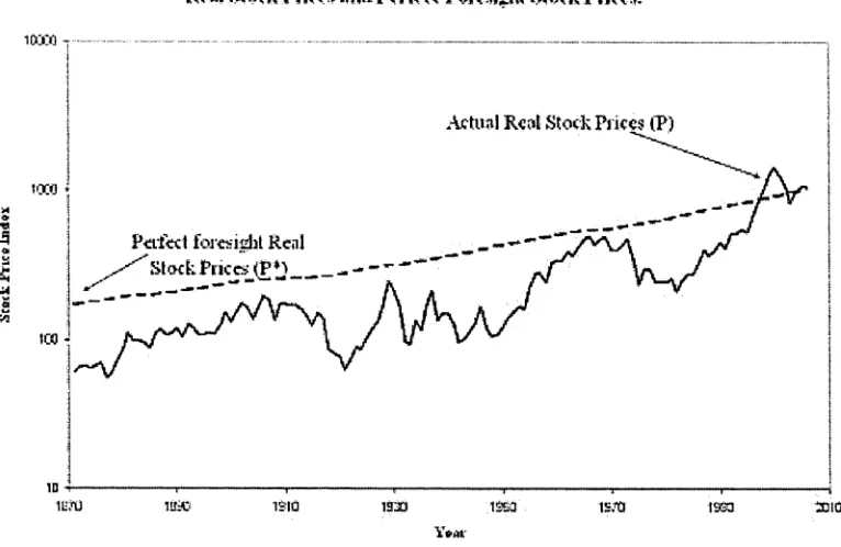
4.2 A look at the d a t a ...36

4.3 Computing the perfect foresight price ...37

4.4 Instrumental v a ria b le s ... 39

4.5 Sample au to co rrelatio n s... 39

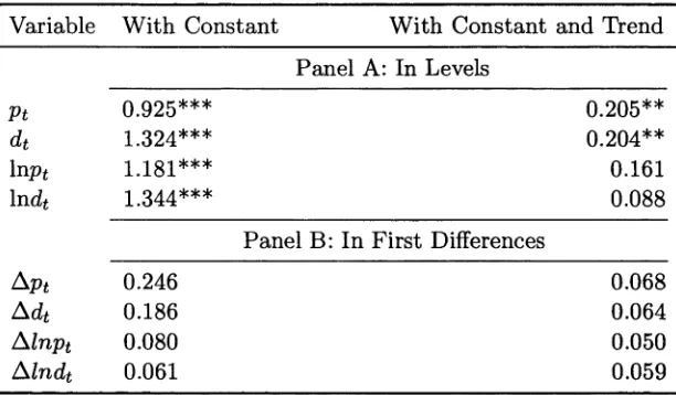
4.6 U n it R o o t T e s t s ...40

4.6.1 Augmented Dickey- Fuller Tests ... 41

4.6.2 KPSS T e s t s ...42

4.7 Inducing stationarity in stock market d a t a ...43

4.8 S u m m a r y ... 46

5 E m p iric al R e su lts an d A nalysis 47 5.1 Overview ... 47

5.2 Computing Unconditional V ariance... 47

5.3 Unconditional Variance Bounds Tests ...49

5.4.1 T h e im portance of conditioning in form ation ... 51

5.4.2 Subsets of conditioning inform ation ...51

5.4.3 D i v i d e n d s ...51

5.4.4 T h e Real Interest R a t e ... 52

5.4.5 C onsum ption G r o w t h ... 53

5.4.6 U nconditional and C onditional Variance bound t e s t s ... 55

5.5 S u m m a r y ... 56

List of Tables

4.1 Summary Data Descriptive S ta tis tic s ... 36

4.2 Sample Autocorrelations for Levels and First Difference of Stock Market Data 40 4.3 ADF Test Statistic for Stock Market D a t a ...42

4.4 K.P.S.S. Test Statistics for stock market d a t a ... 44

4.5 ADF Test Statistics for Differenced Stock Prices in L e v e ls ... 44

4.6 ADF Test Statistics for Log Differenced Stock P r ic e s ... 45

5.1 Unconditional Variance Bounds Tests ... 50

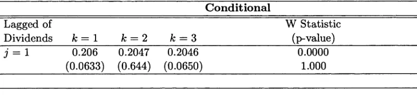
5.2 Conditional Variance Bounds Tests - Real D iv id e n d s... 52

5.3 Conditional Variance Bounds Tests -Real Interest R a t e ... 53

5.4 Conditional Variance Bounds Tests -Consumption G ro w th ...54

L is t o f F ig u re s

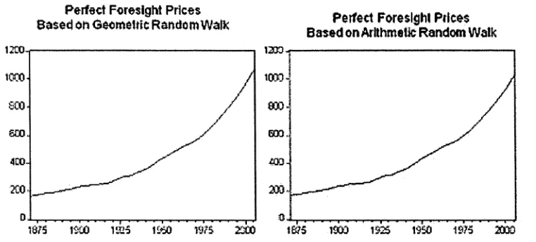
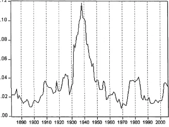
4.1 Annual U.S. Real Stock Prices and Perfect Foresight Stock Prices, 1871-2006 37 4.2 Comparing Two Alternative Perfect Foresight P r i c e s ... 39

C h a p te r 1

I n t r o d u c t i o n

This thesis examines the excess volatility debate using a novel multivariate hypothesis

testing methodology and applying it to annual U.S. stockmarket data. The main thrust of

the literature attem pts to answer this basic question: are fluctuations in stock prices jus­

tified by changes in their fundamental determinants? In an efficient market with rational

investors, stock prices are forward-looking variables that reflect anticipated changes in div­

idends as well as incorporate all relevant information. Hence, their volatility should reflect

investors' expectations of changes in the determinants of stock prices. Given a model of

stock prices, market efficiency places restrictions on the relative volatility of stock prices,

which can be tested to yield insight on the validity of the underlying model. Shillcr (1981)

and Porter and LeRoy (1981) independently investigate this issue and find overwhelming

evidence of excess volatility in stock prices.

If investors arc rational, the stock price should equal the present value of the stock’s

expected dividend stream. By assuming that dividends follow a stationary stochastic

process, it is possible to derive an upper bound for the variance of that stock price based

on the subsequent stream of dividends.

The present value model with constant discount rates, as introduced by Miller and

Modigliani (1961), defines stock prices as the present value of rationally expected future

dividends:

pi = Y,

w here r is th e con stan t discount rate, dt is dividend a t tim e £, where agents base th eir ex p ectatio n s conditional on It , the unobservable vector of inform ation set a t tim e t.

T h e perfect foresight price is th e ex-post rational price w ith perfect inform ation ab o u t fu tu re dividend stream .

r f = £

d t + T

ÜT7T

w here dt is th e realised dividend at tim e t. T he efficient m arkets hypothesis sta te s th a t, u n d er th e assum ption of ration al expectatio ns, th e expected dividend stream should be equal to th e realised dividend stream :

Pt = E t \p*t \It) , (1.3)

w here Et refers to th e m ath em atical ex p ectation conditional on inform ation available a t tim e t. A direct im plication of th e efficient m arkets hypothesis is th a t pt equals p*t

plus a forecast error term , which is orthogonal to p*. O therw ise, th e forecast would not be optim al.

P*t=Pt + u t (1-4)

Hence, they differ by an u n predictable random error, ut which m easures th e im pact on p* of inform ation not available a t th e tim e th a t th e expectation s are formed.

Taking the variance on b o th sides of equation (1.4),

Var(p*t ) = V a r (pt + u t )

V a r ( p * ) = V a r (pt) + V a r (ut ) + 2Cov (pt , u t)

Var {pi) = Var (pt) + Var (ut) (1.5)

Var(p*t ) > Var (pt) . (1.6)

Equation (1.6) therefore places an upper bound on the variance of the observed price

series, under the assumption that prices arc formed according to equation (1.1). This is

the best known of the three variance bounds that Shillcr (1981) developed in his paper

and it forms the basis of most studies in the excess volatility literature.

This simple variance bounds inequality condition can be stated in term of a null hy­

pothesis that involves an inequality constraint of the following form.

Var (p*) — Var (pt) > 0 (1.7)

The extensive literature on variance bounds tests has highlighted that its econometric

implementation is not as straightforward. In fact, any variance bounds testing approach

must tackle the following issues:

• The stationarity properties of dividend and stock price series to ensure that the

variance bounds tests arc robust to the presence of unit roots.

• The computation of p* or an alternative measure of the variance implied by the

present value model.

• Tests of significance of the results.

This follows from Gilles and LcRoy (1991) and Cochrane (1992) who argue that all

econometric tests arc a joint test. The rejection of any null hypothesis could be due not

only of the market efficiency hypothesis or present value model of stock prices, but also

from a failure of the maintained assumptions underlying the econometric test itself.

Our research suggest that, within a proper statistical inference framework, i.c. the

multivariate inequality constraints approach, one is able to reject the claim that the lack

restrictive assumption of constant discount rate, our variance bounds inequality conditions

arc not rejected by the data, unconditionally and conditionally.

This thesis aims to offer an alternative approach based on multivariate inequality re­

strictions hypothesis testing framework since the null hypothesis of interest is an inequality

variance condition. In addition, the framework of Boudoukh, Richardson and Smith (1993)

permits the use of conditioning information in order to restrict the information space un­

der which conditional variance bounds can be tested. It is widely established in the excess

volatility literature by Marsh and Merton (1986) and Klcidon (1986) that unconditional

variances are not well defined for unit root processes. In this study, stationarity of the

stock prices series is achieved by appropriate differencing.

When using conditional information, as dictated by economic theory, the econometric

results, also support the variance bounds theorems. When conditioned on past dividends,

the real interest rate and consumption growth, the multivariate inequality tests fail to find

excess market volatility. It is also found that failing to account for stationarity will lead

to a rejection of the variance bounds.

Following this introduction, the thesis is divided into four main chapters and a conclu­

sion. Chapter 2 covers the excess volatility literature in terms of the different approaches

to the econometric issues raised by Shillcr (1981) and LcRoy and Porter (1981). Then, a

brief overview of the multivariate inequality methodology, as applied to hypothesis testing

is provided. The main aim is to bring together the two strands of literature in order to

address the excess volatility debate and develop testable implications for conditional vari­

ance bounds. Chapter 3 develops a new variance bounds inequality condition and applies

the multivariate inequality methodology to test the validity of conditional and uncondi­

tional variance bounds. Chapter 4 examines the properties of the annual data provided

by Shillcr, in order to access its suitability for our volatility bounds tests. We also inves­

tigate the suitability of alternative differencing strategies in terms of achieving stationary

series. Chapter 5 applies the multivariate inequality methodology to annual U.S. data and

analyzes the results. The results from the study yield unequivocal evidence in favour of

conditional and unconditional volatility bounds. We find no evidence of excess volatility

C h a p te r 2

L itera tu re R e v ie w

2.1

O v e r v ie w

Since the the seminal work by Shillcr (1981) and LcRoy and Porter (1981), variance bounds

tests have been the focus of controversy in the literature. Both papers, using the present

value model of stock prices, found that stock prices arc too volatile to be consistent with

the present value of rationally expected future dividends discounted by a constant rate.

The violation of Shillcr’s variance inequality condition has been interpreted as rejection of

the efficient market hypothesis. Cochrane(1991) argues that volatility tests are only tests

of specific discount rate models and specific dividend models. Other extensive surveys of

the literature can be found in West (1988b), Gillcs and LcRoy (1991) and Gurkaynak

(2008).

Studies which favour Shillcr’s conclusion include Mankiw, Römer and Shapiro(1985),

Campbell and Shillcr (1987, 1988, 1989), Potcrba and Summcrs(1986) and West (1988a).

Several studies have called into question the validity of Shillcr’s results for a variety of

reasons, notably Flavin (1983), Kleidon (1986), Marsh and Merton (1985), Hoshi (1987),

Cochrane(1991), Cuthbertson and Hyde (2002), Heaney (2004) among others. In sum­

mary, after two decades of research, the evidence on the violation of variance bounds rests

largely on a myriadc of model assumptions and weak statistical tests. Not surprisingly,

several authors have expressed a perception of futility when reviewing the inconclusive

(1991), LcRoy(2005) and Cochranc(1991) for extensive surveys of the literature.

The first half of this chapter examines the various themes present in studies undertaken

in the excess volatility literature. The main themes arc:

• The non-stationarity issue of stock market data and how they deal with it.

• Assumptions about the dividends process.

• Different classes of variance bounds theorems - conditional vs unconditional bounds.

• Computation of perfect foresight prices: theoretical and econometric issues.

• non-constant discount rates.

The chapter is organized as follows. Section 2 critically surveys the excess volatility

literature in terms of the econometric issues raised by previous studies. Section 3 briefly

introduces the multivariate inequality constraints literature and the subset that allows us

to test linearity restrictions implied by variance bounds theorems. This thesis adopts two

unique approaches to assess excess volatility by applying a new econometric methodology

to test the variance bound inequality conditions typically found in the literature. 1'hc

study will generate several benefits. Most important is the additional insight into the

excess volatility debate by examining rolling variances bounds that are robust to unit

roots.

2.2

T h e E x c e s s V o la tility L ite r a tu r e

2.2 .1 T h e n o n -sta tio n a r ity issu e

Despite the intuitive appeal of the variance inequality just stated, empirical implementa­

tion is far from straightforward. An important econometric problem is th at if the uncondi­

tional population variances change over time then sample variances, not being consistent

estimates of the population variances that arc subject to the inequality, are unintcrpretable

from the viewpoint of the variance-bounds theorems. Sample variances are of interest only

if some data transformation can be found which ensures that the relevant variables arc

Shillcr (1981) and LeRoy and Porter (1981) carried out their studies based on the

assumption that the prices and dividends series arc trend stationary. Nelson and Kang

(1984) show that doing so docs not resolve the non-stationarity issue if the data series still

contain a unit root.

Heaney (2002) describes Shillcr (1981) approach to achieving stationarity in the stock-

market data as follows. The stock prices and dividends series are detrended by a long-run

growth factor, A^_/ = (1 + g)l~l , where g is rthc growth rate and T is the base year of

the used stock price index, so that at t = T nominal price equal real growth-adjusted price.

The growth factor is estimated by regressing the natural log of stock prices on an intercept

and a time trend, i.c. pt = c + ßt -1- £t and setting A = . This involves dividing equation

(1.1) by Xf~T and multiplying it by j&fr-After defining Aq = ^ and 7 — y+f 85 the

discount factor for the detrended data series, the following relation can be derived:

oo oo

Pt =

£ (

T = 1 T = 1

The growth-adjusted p and d series arc given by

p t _ Pt

(1 + g)t~T

Dt

Dt

(1+ g)l- T

The growth rate is defined as being less than the discount rate to ensure a finite price.

The discount rate is calculated as the ratio of the mean growth-adjusted real dividend o

the mean growth-adjusted real stock price index: f — E (d) / E (p) .

The distributional assumptions of the first generation tests have been questioned by

many. (Flavin, 1983; Klcidon, 1986, Marsh and Merton, 1986; Durlauf and Phillips, 1988).

In particular, Shillcr (1981) and Porter and LeRoy (1981) assume that both dividends and

stock prices are trend stationary and use different detrending techniques before computing

the point sample variances of the 2 stock prices. Shillcr (1981) divides his data scries by

a long-term growth rate while LeRoy and Porter (1981) reversed the effect of inflation

and retained earnings on dividends and stock prices using an algorithm to remove trends.

Pt =

However, when such series have unit roots, sample means and variances do not exist even

after detrending, and therefore it is not valid to use the computed sample moments as

a estimates of population moments. Flavin (1983) also argues that the sample variances

will be biased due towards rejection of the null hypothesis due to the presence of serial

autocorrelations in the actual stock prices and computed perfect foresight stock prices.

Most studies have undertaken formal tests for unit roots and the second generation

variance bounds tests allow for non-stationartity of dividends and stock prices. Despite

this, there has still been conflicting evidence on excess stock price volatility. LeRoy and

Parke (1992) use price-dividend ratios and assume that the transformed series is stationary.

However, Balkc and Wohar (2005) apply augmented Dickey-Fuller tests to similar data

but fail to reject the null hypothesis of a unit root in the log price-dividend ratio.

Following Shillcr (1981) and LeRoy and Porter (1981), Grossman and Shillcr (1981)

relax the assumption of a constant discount factor and argue th at fluctuations in discount

factors are related to fluctuations in aggregate consumption. They conclude that even

under perfect foresight, the large fluctuations in stock prices between 1949 and 1979, can

not be explained by the fluctuations in aggregate consumption and dividends. However,

if the stock prices series are non-stationary, their attem pt to induce volatility in the price

series is meaningless, as Klcidon (1986) has demonstrated. In LeRoy and Porter (1981),

their test is essentially a vector autoregression (VAR) based test of the market fundamental

prices. It is very similar to the approach in Campbell and Shillcr (1987, 1988, 1989).

Campbell and Shillcr (1987, 1988a,b), using a VAR methodology, investigate a number of

models of equilibrium returns, including the models considered in this paper, finding that

the present valuation model of stock prices is rejected when each of the excess returns,

volatility and consumption models is adopted. In addition, Azar (2004) re-examines the

cointegrating relationship between real dividends and real stock prices and fails to reject

the null hypothesis of no-cointcgration.

Marsh and Merton (1986 ) argue that dividend smoothing most likely causes the divi­

dend data to be non-stationary. Ackert and Smith (1993) suggest that focusing entirely on

dividends omits many other important components of returns such as share repurchases.

volatility problem.

Heaney (2004) applies Shiller’s methodology to the Australian data and finds excess

volatility. However, using an alternative form of computing the perfect foresight price

scries, the severity of the violation is lessened.

Campbell and Shfiler (1987), assuming that dividends are characterized by an arith­

metic unit root, remove the linear stochastic trend in prices by using pt — ß (l — ß )~ l dt

in computing their variance bounds. As a critique to Campbell and Shillcr (1987). Yuhn

(1996) finds evidence of a non-linear cointegration relationship between the prices and

dividend series. Using an error correction model, he finds that forecast errors in the cur­

rent period arc not transmitted to next period stock prices, implying that current stock

prices reflect all available information on market fundamentals.

2 .2 .2 M o d e lin g o f th e d iv id e n d p r o c ess

West (1988b) categorizes variance bounds studies based on whether the tests arc asymp­

totically valid with a arithmetic unit root or with a geometric unit root. In the former

case, following Klcidon (1986), dividends can be assumed to follow the following process1:

dt = padt-1 4- r]at, (2.1)

where r]at is an error term that is independently and identically distributed with a zero

mean and finite variance cri; . Under the assumption that pt arc set according to equation

(1.1), this implies that:

pt = PaPt-1 + CLJIat, (2.2)

where a = Therefore, the implicit assumption made about the stationarity

nature of the dividend process has direct implications for the stationarity properties of its

corresponding stock prices.

An alternative assumption is that the dividend process follows a geometric random

walk process so th a t the logarithm of real dividends can be expressed as:

In dt = fid + lnd*_i + Tjg t , (2.3) where rigt is an error term th a t is independently and identically d istrib u ted w ith a zero m ean and finite variance . Klcidon (1986) s ta te s th a t th e im plied stock prices is given by:

(^)

where r is th e co n stan t discount ra te and g is th e geom etric grow th ra te of dividends, given by (1 + g) = exp _{Md +} &

% (Klcidon (1986)). In order for dividends to converge to

a finite sum, r m ust be g reater th a n g. According to W est (1988b), studies th a t assum e an arith m etic u n it process for dividends include M ankiw et al (1985), C am pbell and Shillcr (1987) and W est (1988a). Conversely, studies th a t conduct variance bounds tests based on a geom etric random walk in dividends include Klcidon (1986), C am pbell and Shillcr (1989) and LcRoy and Parke (1992) am ong others. In this study, we follow Klcidon (1986) and assum e t h a t dividends follow a geom etric random walk in th e derivation of our perfect foresight price series.

2 .2 .3 C la sses o f V arian ce B o u n d s T h e o r e m s

T his subsection docum ents some of th e a ltern ativ e variance bounds theorem s p u t forw ard in th e litera tu re .

M ankiw , Röm er and Shapiro (1985) proposed an altern ativ e unbiased tests of variance bounds th a t do not rely on calculating the ex post ratio n al prices, which arc unobservable. T hey come up w ith th e following variance inequalities:

Eo(p*t - p ° t) 2 > E 0 (p*t - p t)2 (2.5)

where p is defined as the naive forecast of stock prices based on dividends information

available to agents at time t Assuming extrapolative and myopic expectations for the

forecast of dividends, we get

Then, pj is defined as

d>t-{-i — di Vz (2.7)

(2.8)

West (1988a) derives an inequality that the variances of innovations in actual stock

prices must be less than or equal to the variance of the innovations in the forecasted

present value of dividends based on a smaller subset of information available to the market.

Therefore, even if dividends and stock prices arc integrated of degree one, the innovations

would have finite variances.

LcRoy and Parke (1992) attem pt to resolve the non-stationarity issue by dividing

dividends into stock prices. Given that current dividend at time t is in the information

set It, the following variance bounds condition can be derived:

Var (pt/dt) > Var (pt/ d t) (2.9)

A recent paper by Engel (2005) argues that when expressing stock prices in first differences,

the Shiller inequality condition is reversed. In particular, he shows that:

Va r ( p t - p t -i) > V a r (p*t - p*t_x) (2.10)

Upon further scrutiny, equation (2.10) contradicts the rational expectations model. To

illustrate this, consider equation (1.4) which forms the basis of the efficient markets hy­

pothesis that underlying all valid variance bound theorems:

P t = P t + u t (2-11)

cqua-tion (2.11) and then takes variances on both sides, then the equality condicqua-tion in equacqua-tion

(2.11) may no longer holds.2 As a result, there is no guarantee that V ar (p* — p*_i) >

Var (pt — p t -1) • Indeed, Engel (2005) analytically confirms that this is the case with equa­

tion (2.10). Therefore, Engel’s new variance bounds arc not at odds with the empirical re­

sults provided by Shiller (1981). Klcidon (1986) has warned that comparing Ear(p*|p*_^)

with Var(pt- \ \pt-j) as it will lead to misleading interpretations.

C o n d itio n a l v a r ia n ce b o u n d s

The actual stock price pt at time t depends on the realization from the distribution of the

error term at time t. Therefore, the variance bound has to hold cross-sectionally, as the

information available at time t — 1 determines the possible values of the present value of

dividends. Therefore, the variance bounds relationships must hold in terms of conditional

variances, i.e.

Var (Pt\It-k) > V a r ( p t \It- k),

where It is the conditioning information available to agents at time t — k. In West

(1988a), H t is defined to be the information set consisting only of current and past divi­

dends. H t = {dt, dt~l, ...} and Ht C I t . Define pt as the price that prevails conditional

on H t :

Pt = Et (p t* |H t )

Assuming that It is at least as informative as H t, i.e. H t C I t , the rule of iterated

expectations implies that:

pt = E t (Pt\Ht),

but the conditional expectation of any random variable is less volatile than the variable

itself. This implies that:

-Var (Pt) > V a r (pt)

Kleidon (1986) points out that the basic unconditional variance bounds relationship

holds cross-scctionally since information available at time t — 1 restricts the possible values

of present value of future dividends in different states of the economies at any given time

t. In general, this implies the following conditional variance bound relationship for k < oo:

Var(p*t \It_ k) = Var { pt \It_k) + Var { ut\It- k) (2.12)

Var (p*t \It_k) > Var (pt \It_k) , k = 0,...,oc, (2.13)

where It~k G It ,and rational expectations requires that Var (ut \h-k) = 0- Akdeniz

et al confirm the argument made by Kleidon (1986) th at one can not made valid inferences

from unconditional variance bounds. They generate simulated data based on an economic

model that is consistent with efficient market hypothesis and apply it to Shiller (1981)’s

variance test and find it is rejected by the test.

T h e in f o r m a t io n s e t

The fundamental concept of market efficiency relies heavily on the what goes into the

information set. As pointed out by Sentana (1993), the concept of market efficiency is

information dependent, since different information set will lead to different concept of

informational efficiency (i.e. asset prices incorporate all relevant information).

In this sense, variance bound test are attem pts at testing the weak form of efficiency,

as described by Fama (1970). Weak efficiency is where the information set contains lagged

values of the price and dividend scrie,s as well as macroeconomic information such as past

interest rates.

West (1988a) posits that the conditional variance would be smaller when the informa­

tion set It contains additional variables useful in forecasting dt than when the information

2 .2 .4 C o m p u ta tio n o f u n o b serv a b le e x p o st sto ck price p*t

Another controversial issue in the excess volatility literature is the computation of the

perfect foresight price scries, which is determined by the present values model of stock

prices. Following Shillcr (1981) and Flavin (1983), studies that compute an observable

version of the perfect foresight use the following recursion:

Pt =

P*t+ 1 + dt + 1

1 + r (2.14)

subject to a terminal condition that the terminal p^ is the last data point pt- The constant

discount rate used is either computed from real data from the real interest rate over the

whole sample, as in Shillcr (1981, 2003) or incremental values of discount rates of 1 percent

to 5 per cent arc used (as in Klcidon (1986). In Shillcr (1988) criticizes Klcidon’s use of a

discount rate that is lower than that observed in the data.

There has been theoretical issues with the direct computation of the perfect foresight

price, p i by many. Klcidon (1986) points out that, ex-ante, dividends arc uncertain

and there arc several possible paths they can take. Hence, stock prices change as the

probabilities of different dividend paths change as new information are known. Ex-post,

there is no uncertainty and only one path is observed in historical data. By construction,

P(t)* must be smoother than the actual stock prices.

For instance, the computation of p* involves an infinite sum of future dividends. Since

any sample is finite, a terminal condition p \ must be used.

Although pi is not observable, it is known that the ex post rational price is the solution

to the recursive expression:

Pt = ß {Pt+i + dt+ l) (2-15)

that satisfies the condition

lim ß lp*t = 0. (2-16)

t —* oo

This approach has been subject to various criticisms, mainly from Flavin (1983) and

Klcidon (1986). The latter shows that Shillcr’s use of ex-post dividends to construct p*

is incorrect since he is assuming that agents know the future dividend stream at the time

of the stock price valuation. Such dividends depends on different possible states of the

economy. Therefore, the ex-post dividend scries is only one of many possible realizations.

Shillcr (1981) estimates the dividend process recursively by taking thr average growth

adjusted real stock price from the full sample as the prevent value of dividends at the end

of the sample. The price p^ is taken as being the most recent observation and p* is then

solved recursively back to the first observation using the equation:

P*t = 7 {Pt+i + dt)

Heaney (2004) argues that stock prices can be expressed as simple perpetuity rather

than requiring perfect knowledge of the future dividends stream. Under the assumption

that dividends follow a random walk, this implies th at the agents form their expectations

on the basis of the last dividend payment. This follows that p* can be re-written as:

* _ d t -1

PRW t - ~ ~ ~

This version of p* is referred to by Mankiw et al (1985) as a myopic forecast of stock

prices.

Following Amano and Wirjanto (1998), the perfect foresight price is calculated using

Hansen’s (1982) generalized method of moments estimate of a non-linear asset-pricing

equation that allows for time-varying real asset returns. This relaxes the strong assumption

of constant real asset returns and risk neutrality thathave characterise first generation

models.

Other papers have attempted to bypass constructing an observable version of the p*

series altogether. For instance, West (1988a) focus on the variances of innovation implied

by the present value model whereas Campbell and Shillcr (1987, 1989) adopt the VAR

2 .2 .5 N o n c o n sta n t D isco u n t R a te s

From the outset, there has been several attem pts to rationalize the evidence of excess

volatility in earlier studies. One explanation put forward by LcRoy and La Civita (1981)

and Grossman and Shillcr (1981) is th at most of stock prices variability is attributed to

changes in the discount rate. Therefore, if one uses a present value model with constant

discount rate, one would fail to adequately capture the variability in the unobserved stock

prices.

A large proportion of first generation and second generation variance bounds tests

rely on the crucial assumption of constant discount rates. The unobservable p* series are

either generated using an estimated value of ß from the data (for instance, Shillcr (1981))

or reasonable values as implied by economic theory (Klcidon (1986)). In both eases, the

variability in p* is predominantly explained by the variability in the dividends stream,

ceteris paribus.

It has been pointed out that variance bounds tests depend on an implicit assump­

tion of risk neutrality (LcRoy (2005)). LaCivita and LcRoy (1981), using Lucas (1978)

model, show that allowing for risk aversion increase the predicted volatility of stock prices.

Constructing the p* series therefore involves a two-step estimation procedure. Following

Amano and Wirjanto (1998), one can use GMM estimates of coefficient of risk aversion

and the rate of time preference. Then, one uses the consumption and dividend series as

well as a terminal stock price, p r and recursively derive p*. The relaxation of the constant

discount rate is likely to induce less smoothness in the p* scries as well as more variability.

Grossman and Shillcr (1981) compute the perfect foresight price based on asset pricing

model with non-constant discount rate. They use aggregate consumption data to construct

p* for different values of risk aversion. They show that a relatively high value/degree of

risk aversion to ensure that the p* series match the p series. They still find evidence of

2 .2 .6 T e stin g m e th o d o lo g y

As documented in West (1988b), there is a wide range of econometric techniques used

to test the variance bounds theorem in section 2.2.3. Shillcr (1981) make use of simple

point estimates of variances, whereas LcRoy and Porter use a VAR approach that allow

them to obtain standard errors of their estimates. West (1988a) also provides standard

errors of the variances of the innovations of returns. However, none of those tests directly

test the null hypothesis of the inequality constraints implied by the variance bounds.

Monte Carlo simulations of statistical and economic models have been used to test the

variance bounds since Klcidon (1986) demonstrates that the variance bounds should hold

cross-sectionally across different states of the world. Kleidon (1986) simulates several

economics where the dividend process follows a geometric random walk and shows that

across different economies, the variance bounds relationship derived by Shiller (1981) holds

cross-sectionally. Akdeniz et al (2007) replicates Klcidon’s approach by simulating cross-

sectional data from a theoretical asset pricing model that satisfies the rational expectations

assumption. They find that unconditional variance bounds are violating using Shiller’s

approach but conditional variance bounds arc not rejected by the simulated data. LcRoy

and Parke (1992) use Monte Carlo experiments to generate perfect foresight prices which

arc derived from a geometric random walk dividends process. Estimates of variances from

price-dividend ratios arc then computed from an analytical closed form expression. LcRoy

and Parke (1992) arc unable to reject the variance bounds condition implied by equation

(2.9).

2.3

T he M ultivariate Inequality C onstraints Literature

One recurrent criticism of Shiller’s original work is the absence of test of significance of his

point variance estimates. Similar criticisms arc applicable to Mankiw etal( 1985), LcRoy

and Parke (1992) and any empirical studies that have replicated Shillcr’s variance bound

2.3 .1 B a ck g ro u n d

The multivariate inequality restriction methodology seems suited to examine the excess

volatility debate. The variance bounds theorems described in the previous sections, pro­

vide apriori information about the sign of the variance bounds conditions implied by

rational expectations and the present value model of stock prices. Therefore, the main

appeal of the multivariate inequality constraints test is that it provides a statistical test

of the validity of a priori signs of the parameters where such a priori beliefs point to

an inequality restriction, rather than an equality restriction (Wolak (1989)). Within the

multivariate inequality constraints framework, moments conditions are jointly tested so

that potential correlations among the moment conditions axe taken into account.

This thesis draws upon a branch of the literature on statistical inference in which

multiple inequality constraints arc been tested as the null hypothesis. 3 In such eases,

incorporating this a priori information in the hypothesis testing of the parameters of

interest would yield more relevant inference. To illustrate this, consider the following null

and alternate hypotheses:

Hq : Rß > r versus Ha : ß € Rh ,

where Rß > r is a vector of inequality conditions being tested. The test involves computing

an unrestricted estimate of ß and a restricted estimate of ß subject to R ß > r.

Using the results provided in Wolak (1989), a Wald test statistic, W , can be derived.

Such test statistic no longer has an asymptotic \ 2 distribution but is a weighted mixture of

X2 distributions with different degrees of freedom under the null hypothesis (Gourieroux,

Holly and Monfort, 1982). To compute the weights of the test statistic, Kudo (1963)

provides an analytical expression for its special ease. Gourieroux, Holly and Monfort

(1982) use complex numerical simulation. Wolak (1987) derives closed form expression

for the weights for dimensions of the inequality constraints tests less than 5. Koddc and

Palm (1986), however, building on Perlman (1969) propose lower and upper bound critical

values that correspond to a given level of significance without calculating the weights. For

a given level of significance, the null hypothesis is rejected if W exceeds the upper bound.

Conversely, the null can not be rejected if the test statistic is less than the lower bound.

For values of W between these bounds, Wolak (1989) develops an approximate numerical

method of calculating the weights based on a Monte Carlo simulation.4

2 .3 .2 L itera tu re d e v e lo p m e n ts an d e m p irica l a p p lic a tio n s

The multivariate inequality testing problem has roots in papers by Bartholomew (1961),

Kudo (1963) and Perlman (1969). They focus on the multivariate one-sided hypothesis

testing. Bartholomew (1959) proposes a hypothesis test for ordered alternatives. It was

was expanded by Kudo (1963). The latter develops a multivariate equivalent of a one­

sided significance test. The null hypothesis is that all parameters are jointly equal to zero

against the alternative that at least one parameter is strictly positive under the alternative.

Kudo (1963) applies the methodology to study the impact of development variables on

birth deformity in Hiroshima and Nagasaki.

Yancey, Judge and Bock (1981) develop hypothesis tests that involve a combination of

equality and inequality restrictions in a single test and constrast the critical regions with

the conventional cases of two equality hypotheses. Other notable contribution to the mul­

tivariate inequality literature include Gouricroux, Holly and Monfort (1982) who examine

multivariate one-sided hypothesis testing and investigate the equivalence and differences

between the LR test, the Wald test and the Kuhn-Tuckcr tests. Wolak (1987, 1989, 1991)

generalize the inequality constraints methodology to a wide range of econometric problems

in economics and finance.

The monotonicity of term premiums was reconsidered by Richardson, Richardson, and

Smith (1992) relying on recent econometric techniques for testing inequality constraints on

linear models developed by Koddc and Palm (1986) and Wolak (1989). They combine the

literature on conditional asset pricing models as well as unconditional multivariate inequal­

ity testing to create a testable framework to examine conditional inequality conditions.

They replicate Fama (1984) results and can not refute the liquidity preference hypothe­

sis. In Boudoukh, Richardson, and Smith (1993), the methodology has been expanded in

order to allow moments to be conditioned on a set of instrumental variables, which arc

observable and can be used to further restrict the information set. An appealing feature

of their testing approach is that it does not require a full specification of the infromation.

In order to preserve the inequality conditions being tested, the information vector has to

be constrained to be a positive subset of variables. One of their objectives is to identify

states in which the conditional exante equity premium is negative. Osdick (1998) applies

Boudoukh et al (1993) methodology to test whether the world exante risk premium is

positive. Walsh (2006) tests the CAPM implications on the equity risk premium over

different investment horizons.

2 .4

S u m m a r y

The empirical implementation of variance bound tests has been more complicated than

it appears on the surface. The literature is rife with attempts at ironing out several ar­

eas of controversy, both on theoretical grounds and on econometrical grounds. There arc

a myriad of differences in data modelling assumptions and econometric approaches that

suggest why some variance bounds tests find excess volatility while others do not. Despite

more than two decades of research, the jury is still out on the volatility bounds contro­

versy. The principal issue of stationarity can be resolved by appropriate differencing and

multivariate tests incorporating conditional information can be made by using advances

in multivariate inequality testing literature to conduct valid volatility bounds tests. This

C h a p ter 3

M e th o d o lo g y

3.1

O v e r v ie w

The main purpose of this chapter is to offer an alternative approach to existing tests of

stock price volatility. Most of the focus in the volatility literature has been on alternative

modeling of dividend and stock price processes. A novel feature of this thesis is to explicitly

test the null hypothesis of the variance bound inequalities in an inequality restrictions

framework. If the market is efficient, then the null hypothesis of the testable moment

conditions should not be rejected. One potential problem in the existing literature is that

sample estimates of variances are usually compared and no confidence intervals of the

estimates arc available. This thesis brings together the variance bounds literature into

the modern world of multivariate statistical inference.

This chapter is organized as follows. Section 3.2 derive testable implications of uncon­

ditional and conditional variance bounds conditions that axe valid even if stock prices and

dividends have unit root processes. Section 3.3 describes the multivariate inequality test­

ing methodology that was developed by Boudoukh, Richardson and Smith (1992). Section

3.4 concludes.

3.2

V a ria n ce B o u n d s C o n d itio n s

The present value model defines stock price as the present value of rationally expected

(3.1)

^ E t (dt+T\It)

Pt = § U i

ttt

“

where r is th e discount rate, dt is dividend a t tim e t, where agents base th eir ex p ecta­ tions conditional on It , th e inform ation set a t tim e t.

T he perfect foresight price is the ex-post price w ith perfect inform ation a b o u t fu ture dividend stream .

p't =

1C

Ü+7T

where dt is th e realised dividend. U nder th e assum ption of ratio n al ex pectatio n s, expected dividend stream should be equal to th e realised dividend stream :

p t = E\p*t \It\ . (3.3)

By definition, pt equals p*t plus an erro r term , which is orthogonal to p*t .

Pt = P t + u t (3-4)

U nder ratio n al expectations, it m ust be th a t:

V a r (p*) > V a r (pt) . (3.5)

E q u atio n (3.5) therefore places an upper bound on th e variance of th e observed price scries, under th e assum ption th a t prices are form ed according to equation (3.1). T h ere is w idespread evidence in th e litera tu re th a t equation (3.5) can not be d irectly tested . Therefore, one m ust resort to m aking su itable d a ta transform ation s to th e pt and p* scries to induce statio n arity.

To derive a variance bounds condition th a t is theoretically consistent w ith equation (2.11), one m ay su b stra c t p t- i from b o th sides. T his implies:

Taking unconditional variance leads to:

V a r (p* - p t _i) = V a r ( p t - p t- i ) + V a r (ut ) (3.7)

Under the assumptions that Va r (ut \pt) = 0 and Cov ( u t , u t-1) = 0, we arrive at the

following unconditional variance bounds condition:

V a r {p* - p t - i ) > V a r {pt - p t - i ) (3.8)

In order obtain valid sample variance estimates from testing equation (3.8), we require that both (p* — p t -1) and (pt — P t - 1) to be stationary, even if p* and pt may not be.

Given that there is overwhelming evidence of the random walk nature of the actual stock prices given by p t , we need to formally test that (p* — p t - i ) also satisfies the stationarity property. Assume that p t has a unit root in levels1 and is given by:

p t = p t -1 + et, (3.9)

P t - P t - i = et (3.10)

where et is i.i.d. (0, er;?). Substituting (3.10) into equation (3.6) yields:

p * - p t - \ = et + u t . (3.11)

Therefore, on theoretical grounds, one expects the sum of two stationary processes to be stationary as well. In Chapter 4, the stationarity properties of the data scries used in computing variances will be investigated in more depth.

An alternative specification of rational expectations assumption that defines the rela­ tionship between the actual stock price and the perfect foresight stock price is to express equation (3.3) as follows:

Pt = Pte£t■ (3.12)

It is straigh tforw ard to show th a t taking expectations of equation (3.12) will yield equation (3.3).

Taking logs on b o th sides yields:

\ n p l = \ npt + Eu (3.13)

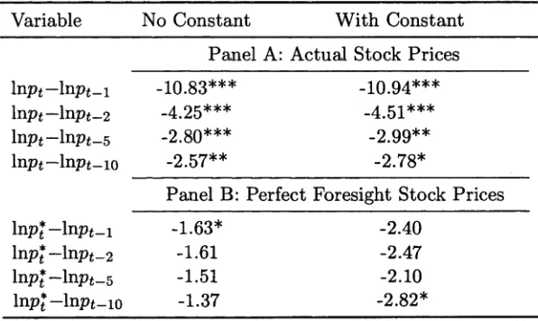
where e f i . i . d (0, er^). T he log specification indicates a m ultiplicative error stru c tu re , com ­ pared to an additive error s tru c tu re as in equation (3.4). To induce statio n arity , we sub- stract, ln p t_ i from b o th sides of equation (3.13). T his yields:

hip* - ln p t_ i = \ n p t - ln p t_ i + et , (3.14)

Taking variances on both sides gives rise to th e following variance inequality condition:

V a r (Inp* - ln p t_ i) > V a r (Inp t - I np t- i ) (3.15)

T his can be generalized to conditional variances of the form:

V a r (Inp* - ln p t_ i |J t_ i ) > V a r (Inp t - ln p t_ i | / t_ i ) . (3.16)

K lcidon (1986) argues th a t the variance bounds in equation (3.10) has to hold cross- scctionally since th e inform ation set I t- \ d eterm ines th e possible values of th e present value of dividends stream . Therefore, th e variance bounds inequality should also hold for conditional variances:

V a r (Inp* - \ n p t- \ \ I t- k ) > V a r ( ln p t - \ n p t_ k\It_ k) . (3.17)

where I t- k denotes th e conditional inform ation set a t tim e t — k.

V ar (p* - p t - j \ I t- k) > V a r ( p t - p t - j \ I t - k )

t-3 t - j

V a r ( p *- p t - i \ I t- k) - Var (pt - p t - j \ I t- k) > 0

(3.18)

(3.19)

The fundamental hypothesis behind the volatility literature is whether this condition

is ever violated. Secondly if violations take place, what arc the instruments that arc

responsible? Third, has there been historical episodes where the variance bounds were

violated? Are there time horizons implications?

Notice in equation (3.19) we subtract pt-j from both sides of the inequality condition.

This is necessary to preserve the inequality. If the first differences of p* and pt were used

instead, it possible, as shown by Engel (2004), th at the inequality is reversed. There has

also been some debate regarding the plausibility of the empirical results using reasonable

parameter values. Nevertheless, it remains an empirical question as to whether this con­

dition actually occurs. In this section, the testable inequality restrictions implied by the

variance bounds condition arc deduced.

Due to the nature of the condition (i.c. in order to maintain the initial inequality con­

dition and not reverse the sign in equation (2.8), only instrumental variables, which arc

non-negative for all t(dcnotcd by z f) are used. Such instruments can include the level of

real interest rate, dividends, or past volatilities of stock prices and so forth. These instru­

ments ought to be based on existing economic theory, which provides some information

about the stock volatility.

The set of instruments, z f , arc non-negative so that multiplying both sides of equation

(2.9) will not change the sign. Any random variable zt can be separated into two positive

variables, = max(0,Zf) and z%t = max (0, —zt),which captures all postive states of

the world. Consistent with Boudoukh, Richardson and Smith (1993), each instrument is

normalised by dividing through by the expected value of z-t to yield z+ for each instrument.

Therefore, using an instrumental variables approach, it is possible to rewrite equation

(3.20)

E

t - j V a r (p* - p t_j) <g> 2+.J - V a r (pt - p t__j) <g> z£_j £ <8> > 0

Rc-arranging (2.9) and applying the law of iterated expectations,

E

t - j

E

[ V a r {p*t - p t - j ) - V a r (pt - p t- j ) } <g> - 0ez+

I Var (p* - p t - j ) - V a r (pt - p t- j)} ® z ^ - 0£Z+

0,

0

(3.21)

(3.22)

where

0ez+ E £ < g > Z +_5 > o (3.23)

Equation (3.23)2 provides a set of moment conditions for which the vector of parame­

ters, Qe z + , is to be estimated. The various benefits of this approach are as follows. There

is no need for an explicit model of conditional expectations. The stationary and ergodity

assumptions are implictly satisfied since we are computing variances of lagged difference

of the stock prices, not the level of stock prices. There is also an existing literature on the

determinants of stock price volatility, which would be useful candidates as instrumental

variables. Here, there is no assumed functional form, sos this is not a potential problem.

Finally, the multivariate inequality restrictions framework, developed by Wolak and used

by Boudoukh et al (1993) is perfectly suitable to analyse the hypotheses. In particular, the

inequality restrictions implied by the variance bounds condition can be jointly tested and

will take into account any correction across the estimators 0 e z + . For example, in evaluating

the significance of the estimators, the relevant factors are no only the magnitudes of the

cstimaccs but also whether these magnitudes are consistent with the covariance matrix of

e e z + .

2It is straightforward to show that taking unconditional expectations implies that V a r ( X ) =

3 .3

E c o n o m e tr ic M e th o d o lo g y

In this section, the test statistic for testing inequality restrictions is described. It follows

closely Boudoukh et al (1993), which draws upon Wolak (1989) and Koddc and Palm

(1986).

Suppose that there arc T observations on the lagged variances Var (pi — Pt - j ) —

Var (pt — Pt - j ) and a N-vcctor . Assume these random variables arc stationary and cr-

godic, with finite variances. Let the variance-covariance marix of the sample moment

vec-, be defined as Q. As described

tor, f Y j = \

{^ar

}

by Wolak (1989), this matrix can take quite general forms and can account for cross-

section, autocovarianccs or hetcroskcdasticity in the series.

The restrictions given in equations (3.21) and (3.23) can be written as a system of

N-momcnt conditions:

E t-j

E t-j

I P a r (pi - pt-j ) - V a r (pt - pt- j) }

{ V ar (p*t - pt-j) - Var (pt - pt- j ) } z%t_5

0,

0 , V j ,

The null and alternate hypothesis can be expressed as follows:

Ho : 0„+ >0 V* = 1,--- ,N. (3.24)

e z t

versus

Ha ■ e c, t € R n .

With respect to testing the hypothesis in (3.24), the first step is to estimate the sample

1 T

° e z += T ^ 2 [ { V a r (Pt - P t - j ) ~ V a r ( P t - P t - j ) } z £ - j , Vj, z = 1, • • • , AT. (3.25) £=1

There is no restriction on the sign of the difference variances. In other words, they

may be negative to sampling error or the possible rejection of the null hypothesis. It

is important to note that the vector 0£z+ is asympotically normal wiht mean 0£Z+ and

variance-covariance matrix Q. The Q can be estimated using Newey and West (1987)

lictcroskcdastic-consistcnt techniques.

Under the null hypothesis restriction in (3.24), the parameter estimates must be non-

negative. Following Perlman (1969) and Wolak (1989), estimates arc derived under the

restriction by minimising the deviations from the unrestricted model:

min (e£z+ - e £Z+^j (&£Z+ - 0 £z^ j

subject to 0£Z+ > 0.

Let Qez be the solution to this quadratic program.

The aim is to test how close the restricted estimates 0£Z+ arc to the unrestricted

estimates 0£z+. Under the null, the difference should be small. In particular, the test

statistic is given by:

W = T (oez+ - 0CZ+) ' ST1 - i)ez+) (3.26)

Wolak(1989) shows that W docs no longer have an asymptotic chi-squared distribution

in the presence of inequality restrictions. Instead, the statistic is distributed as a weighted

sum of chi-squared variables with different degrees of freedom. Specifically, the asymptotic

distribution of W is given by:

£ P r [ x i > c ] W ( A r , . / V- f c , p ) , (3.27)

fc= 0

V

1 )

where cG R + is the critical value for a given size and the weight w (^N, N — fc, ^ is

the probability that 0£Z has exactly N — k positive elements and Xo is a point mass at the

As discussed in W olak(1989), calculating the weights for larger sets of restrictions and non-zero estim ato rs covariances becom e analytically in tractab le. As an alternative, K odde and Palm (1986) com pute u p p er and lower bound critical values which do not require calculation of th e weights. T hey arc given by:

a

= ^Pr(x?>c,),

« = \Pr ( x ^ _ ! > Cu) + t P r (x% > ,

where ci and cu arc th e lower and u p p er bounds respectively for th e critical values of th e test. It is necessary to com pute th e weights for values betw een these bounds. W olak(1989) proposes an approxim ate m ethod of M onte Carlo sim ulation to calculate the weights in these eases. A m ultivariate norm al d istrib u tio n w ith zero m ean and c o v a r i a n c e ^ ) is sim ulated. We note th e realised vector from each replication by 0*z+. T h e idea is to find th e vector 0ez+ which solves th e following m inim isation problem:

min (0«+ “ 0«+) (?)

su b ject to Qez+ > 0.

For each replication, th e num ber elem ents in th e N vector 0£Z+ th a t arc g reater th a n zero is counted. According to W olak(1989), th e ap proxim ate weight w (iV, N — k, p ) is th e fraction of replications in which 0£Z+ has exactly N — k elem ents g reater th a n zero.

3 .4

S u m m a r y

C h a p t e r 4

D a ta A n aly sis

4.1

O v e r v ie w

This chapter investigates the stationarity properties of dividends and stock prices data.

First, the raw data employed in this study are described.Particular attention is paid to the

importance of the stationarity properties of the data as they influence the derivation and

use of conditional variance bound tests to be implemented in Chapter 5. Flavin (1983),

Marsh and Merton (1983) and Kleidon (1986) among others, were the first to critique

Shillcr (1981) detrending of his data scries in order to achieve stationarity. Kleidon (1986)

also showed that in the presence of a random walk, unconditional variance bounds arc

undefined.

A critique of the excess volatility literature is that some studies directly assume that

their transformed data is stationary without carrying out formal unit root tests on them.

Doing so may lead to questions about the validity of their empirical results.

The next section briefly investigates the null hypothesis that the stockmarket data

contains a unit root. While the sample size may too small to permit a conclusive test, we

find some evidence consistent with this hypothesis. Then, we conduct a series of unit root

tests on two alternative data transformations and this will decide which variance bounds

4 .2

A lo o k a t t h e d a ta

The stock prices data used in this study consists of annual Standard &; Poor’s composite

stock price index from 1971 through to 2006. It is compiled by Shillcr and updated on

his website. The S&P data is extended back to 1871 by using the data in Cowles (1939).

Nominal stock prices are converted into real terms by deflating the January price of the

stock index with the annual average of the consumer price index (CPI) at 2000 prices.

The nominal dividend series, from 1926, is dividends per share adjusted to index for the

Standard and Poor’s composite index. Prior to 1926, the dividend is also taken from

Cowles (1939). Real dividends arc similarly calculated by dividing the total dividend per

share accruing to the stock price index with the C PI.1

Stockmarket data is generally available on an annual and monthly frequency for the

same length of time. In order t,o avoid dealing with seasonality issues and to enable com­

parison with previous studies, annual data is generally preferred. Moreover, our dataset

extends further to 2006 compared to most studies in this literature, which were undertaken

in the 1980s. This longer time scries will allows us to examine whether the worldwide asset,

price bubble in the 1990s will significantly affect our results.

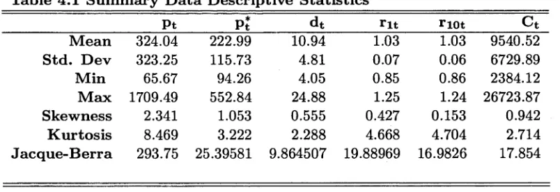
T a b le 4 .1 S u m m a r y D a ta D e s c r ip tiv e S t a tis tic s

Pt Pi d t_______ r it rio t_______ C t

M e a n 324.04 222.99 10.94 1.03 1.03 9540.52

S td . D e v 323.25 115.73 4.81 0.07 0.06 6729.89

M in 65.67 94.26 4.05 0.85 0.86 2384.12

M a x 1709.49 552.84 24.88 1.25 1.24 26723.87

S k e w n e ss 2.341 1.053 0.555 0.427 0.153 0.942

K u r to s is 8.469 3.222 2.288 4.668 4.704 2.714

J a c q u e -B e r r a 293.75 25.39581 9.864507 19.88969 16.9826 17.854

Table 4.1: includes th e m ean, sta n d ard deviation (Std. D ev), m inim um (M in), m axim um (M ax), Skew­

ness, K urtosis and Jacquc-B crra sta tistics for th e real stock prices, th e perfect foresight stock prices, real dividends, 1-year real interest rate , 10-year real interest ra te and real consum ption. All real values arc converted using th e consum er price index.

Table 4.1 presents a summary of descriptive statistics of the annual data used in this

study. Sample means and standard deviations, minimums and maximums as well as