The long-run determination of the real exchange rate. Evidence from an intertemporal modelling framework using the dollar-pound exchange rate

City, University of London Institutional Repository

Citation

:

Pilbeam, K. & Litsios, I. (2017). The long-run determination of the real exchange

rate. Evidence from an intertemporal modelling framework using the dollar-pound exchange

rate. Open Economies Review, 28(5), pp. 1011-1028. doi: 10.1007/s11079-017-9467-7

This is the published version of the paper.

This version of the publication may differ from the final published

version.

Permanent repository link:

http://openaccess.city.ac.uk/17277/

Link to published version

:

http://dx.doi.org/10.1007/s11079-017-9467-7

Copyright and reuse:

City Research Online aims to make research

outputs of City, University of London available to a wider audience.

Copyright and Moral Rights remain with the author(s) and/or copyright

holders. URLs from City Research Online may be freely distributed and

linked to.

R E S E A R C H A RT I C L E

The long-run determination of the real exchange rate.

Evidence from an intertemporal modelling framework

using the dollar-pound exchange rate.

Ioannis Litsios1&Keith Pilbeam2

Published online: 7 October 2017

#The Author(s) 2017. This article is an open access publication

Abstract This paper develops a model of optimal choice over an array of different

assets, including domestic and foreign bonds, domestic and foreign equities and domestic and foreign real money balances to examine the determination of the real exchange rate in the long-run. The model is tested empirically using data from the UK and the USA. The results show that all the coefficients of the model are right signed and significant and consequently financial assets may play a significant role in the deter-mination of the real exchange rate.

Keywords Real exchange rate . Intertemporal model . Asset prices . Vector Error

Correction Model

JEL Classification F31 . G11

1 Introduction

Trying to estimate the equilibrium real exchange rate (ERER) remains a major chal-lenge in modern international finance. A fundamental problem is that the equilibrium real exchange rate is not observable. In addition, according to Rogoff (1996) deviations of the actual real exchange rate from its long-run parity could be linked to the behaviour of macroeconomic fundamentals. In fact, many theoretical models have been construct-ed basconstruct-ed on the premise that the ERER is a function of macroeconomic fundamentals.

Open Econ Rev (2017) 28:1011–1028 DOI 10.1007/s11079-017-9467-7

* Keith Pilbeam [email protected]

Ioannis Litsios [email protected]

1 _{Division of Economics, University of Bradford, Bradford, UK}

2

The standard models in the literature on the determination of the ERER emerge from a simple balance of payments equilibrium equation, the so-called statistical equilibrium; see for example McDonald (2000). The most simple model is the purchasing power parity (PPP) model which implies that the real exchange rate does not change in terms of tradable goods prices but allows for deviations based on price indices made up of both tradable and non-tradable goods. However, the empirical evidence suggests that deviations from PPP can be both substantial and persistent in nature.1Given that PPP is not able to explain the behaviour of the ERER it has been argued that such a measurement can be derived from an economic model in which macroeconomic fundamentals are explicitly present. Different approaches like the behavioural equilib-rium exchange rate (BEER) of Clark and MacDonald (1998) and Driver and Westaway (2004) and the fundamental equilibrium exchange rate (FEER) developed by Williamson (1994) have emerged.

This paper contributes to the literature by proposing an alternative approach to the determination of the real exchange rate in the long-run. As opposed to the current literature, which is heavily based on various extensions of the balance of payments equilibrium real exchange rate equation, our proposed theoretical framework offers a portfolio balance approach to the determination of the real exchange rate in the long run by constructing a two country model with optimizing agents where wealth is assumed to be allocated optimally in an asset choice set that explicitly includes investment in an array of financial assets namely, money, bonds and shares. The model specification introduced in this paper allows the construction of explicit equations for both domestic and foreign real money balances, domestic and foreign bond returns and domestic and foreign share prices to generate a relationship for the determination of the real exchange rate in the long-run. In this paper, we show that the theoretical model that we derive is empirically well supported by using the dollar-pound rate, indicating that asset prices and returns can play a substantive role in the determination of the real exchange rate in the long-run. Although Dellas and Tavals (2013) have recently shown a theoretical and empirical linkage between asset prices and exchange rate regimes, and Fratzscher et al. (2015) provide empirical evidence in favour of the scapegoat theory of exchange rates in understanding exchange rate fluctuations, our approach is to show an explicit link between asset prices, monetary factors and the real exchange rate.2

The rest of this paper is organised as follows: Section 2 presents an intertemporal optimization model, as a contribution to the understanding of the determination of the real exchange rate in the long-run. Section 3 discusses the dataset and empirical methodology for examining the predicted relationship. Section 4 discusses the results from the empirical estimations and Section 5 concludes.

2 The Model

An infinitely lived representative agent (individual) is assumed to respond optimally to the economic environment. Utility is assumed to be derived from consumption of goods and from holdings of domestic and foreign real money balances. The

1

This is the well-known‘PPP puzzle’as labelled by Rogoff (1996).

2

consumption basket is assumed to be a composite bundle of goods produced both domestically and in the foreign economy. The presence of real money balances is intended to represent the role of money used in transactions, without addressing explicitly a formal transaction mechanism. This can distinguish money from other assets like interest bearing bonds or stocks.3The representative agent is assumed to maximize the present value of lifetime utility given by:

Et ∑

∞

t¼0

βt ðCtαÞ1−σ

1−σ þ

X

1−ε

Mt

Pt

η1 _M*

t

P*_t

η2

1−ε

" #

ð1Þ

whereCtis real consumption of a composite bundle of goods,M_Ptt andM

* t

P*

t are domestic

and foreign real money balances respectively, 0 <β< 1 is the individual’s subjective time discount factor,σ,ε,Xare assumed to be positive parameters, with 0.5 <σ< 1 and 0.5 <ε< 1, andEt(·) the mathematical conditional expectation at timet. For analytical

tractability and following Kia’s (2006) suggestion, we assume that ,α,η1, andη2are all

normalized to unity.

The present value of lifetime utility is assumed to be maximized subject to a sequence of budget constraints given by:

ytþ Mt−1

Pt þ M*

t−1

etPt þ

BDt−1 1þiDt−1

Pt þ

BtF−1 1þitF−1

etPt þ

St−1 PSt þdt−1

Pt þ S*

t−1 P S;* t þd*t−1

etPt ¼

Ctþ Mt

Pt þ M*

t etPtþ

BD t Pt þ

BF t etPtþ

StPSt Pt þ

S* tP

S;* t etPt

ð2Þ

whereyt is current real income,M_Pt−_t1 and

M* t−1

etPt are real money balances expressed in

current domestic unit terms (withMt−1andM*_t−1domestic and foreign nominal money

balances respectively carried forward from last period),etthe nominal exchange rate

defined as the amount of foreign currency per unit of domestic currency andPtthe price

index of the composite good consumed domestically.BD_t−1 is the amount of domestic currency invested in domestic bonds att−1 andiD_t−1is the nominal rate of return on the domestic bonds. Similarly,BF

t−1is the amount of foreign currency invested in foreign

bonds att−1 andiF

t−1is the nominal rate of return on the foreign bonds. Both domestic

and foreign bonds are assumed to be one period discount bonds paying off one unit of the relevant domestic currency next period.St−1andS*t−1denote the number of

domes-tic and foreign shares respectively purchased att−1, PS t andP

S;*

t denote the domestic

3_{A direct way to model the role of money in facilitating transactions would be to develop a time-shopping}

and the foreign share prices respectively anddt−1andd*t−1the value of the domestic and

foreign dividends earned.4

The agent is assumed to observe the total real wealth and then proceed with an optimal consumption and portfolio allocation plan. The right hand side of eq. (2) indicates that total real wealth is allocated at time t among real consumption of the composite good (Ct), real domestic and foreign money

balances (Mt

Pt;

M* t

etPtÞ, real domestic and foreign bond holdings (

BD t

Pt;

BF t

etPtÞ, and real

domestic and foreign equity holdings (StPSt

Pt ;

S* tP

S;* t

etPt Þ.

5

The representative agent is assumed to maximize eq. (1) subject to eq. (2). In order to get an analytical solution for the intertemporal maximization prob-lem, the Hamiltonian equation is constructed and the following necessary first order conditions are derived:

βt

Uc;t−λt¼0 ð3Þ

βt

UM

P;t

1

Pt−λt

1

Ptþ

Et λtþ1

1

Ptþ1

¼0 ð4Þ

βt

UM *

P*;t

1

P*_t −λt

1

etPtþ

Et λtþ1

1

etþ1Ptþ1

¼0 ð5Þ

−λt

1

Ptþ

Et λtþ1

1

Ptþ1

1þiD_t

¼0 ð6Þ

−λt

1

etPtþ

Et λtþ1

1

etþ1Ptþ1

1þi_tF

¼0 ð7Þ

−λt

PS_t Pt

þEt λtþ1

1

Ptþ1

PS_tþ1þdt

¼0 ð8Þ

4

It is assumed that the individual collects his dividend first and then goes out in the financial market to trade. In other words, the stock market opens after the realization of dividends.

5

−λt

PSt;*

etPtþ

Et λtþ1

1

etþ1Ptþ1

PS_tþ;*₁þd*_t

¼0 ð9Þ

where λt the costate variable, Uc,t , the marginal utility from consumption and

UM

P;t;UM *_P*;t the marginal utilities from domestic and foreign real money balances

respectively.

It is further assumed that the representative agent consumes according to the following constant elasticity of substitution (CES) composite:

Ct¼ α

1

Θ _Ch

t

Θ−1

Θ _þð1−αÞΘ1 _Cf

t

Θ−1

Θ

Θ

Θ−1

ð10Þ

Where Ch_t;Ctf represent consumption of domestically produced goods and

foreign imported goods respectively. The degree of home bias in preferences is given by parameter α∈[0, 1] and can be perceived as a natural index of the degree of openness of the economy. Parameter Θ> 1 measures the substitut-ability between domestic and foreign goods.

DefiningPh_t and Ptf as the price indexes of domestically produced goods and

goods produced in the foreign economy (all expressed in units of domestic currency), the utility based consumer price index (CPI) of the composite good consumed domestically is given by:

Pt¼ α Pht

1−Θ_þ

1−α

ð Þ Ptf

1−Θ

1

1−Θ

ð11Þ

Given that the nominal exchange rateetis the amount of foreign currency per

unit of domestic currency we can write the domestic price equivalent (Ptf) of the

price index of the goods produced in the foreign economy (P_tf *) asP_tf ¼Ptf *

et and

the foreign currency equivalent of the price index of domestically produced goods (Ph_t) asPh*_t ¼Ph_tet.

Following Galí and Monacelli (2004) a simplifying assumption is introduced namely that there is no distinction between foreign CPI (P*_t) and the price index of the goods produced in the foreign economy (Ptf *) i.e. Ptf * ¼P*t.6 The intuition of

this is that PPP does hold for foreign (tradable) goods. This is not the case however for the domestic aggregate CPI. Assuming that the price index of domestically (non-traded) produced goods increases (given P*

t;P f *

t ) domestic

con-sumers move towards foreign goods and a nominal depreciation is induced. Given the nominal depreciationPtf will increase but given its compositionPtwill increase

more that the nominal depreciation i.e. PPP fails to hold.

6

Consequently, the terms of trade Tt and the real exchange rate qt are defined

respectively as:

Tt¼

Ptf

Ph

t

¼

P_tf * et

Ph

t

¼ Ptf *

etPht

¼Ptf *

Ph* t

ð12Þ

q_t¼

P*_t et

Pt

¼ P*t

etPt

ð13Þ

qtdenotes the real exchange rate defined asqt¼ P*

t

etPtwherePtandP

*

t the price indexes

of the composite bundles of goods consumed domestically and in the foreign economy. A rise inqtrepresents a real depreciation while a fall represents a real appreciation.

The static optimal allocation of total (composite) consumption leads to the following symmetric isoelastic demand functions for both domestic and foreign goods respectively7:

Ch_t ¼α Tt

qt

Θ

Ct ð14Þ

C_tf ¼ð1−αÞð Þq_t −ΘCt ð15Þ

Rewriting eq. (14) and eq. (15) in terms of real total consumption of the composite bundle consumed in the domestic economy leads to eqs. (16) and (17):

Ct¼

Ch

t

α Tt

qt

θ ð16Þ

Ct¼

Ctf

1−α

ð Þq−_tθ ð17Þ

Dividing eq. (5) by eq. (7) and using eq. (3) yields eq. (18):

UM *

P*;t

þUC;t 1þitF

₋1

q_t¼UC;tqt ð18Þ

Equation (18) implies that the marginal benefit of holding additional foreign real money balances at t must equal the marginal utility from consuming units

7

of the domestic composite bundle of goods at time t. Note that the total marginal benefit of holding money at time t is equal to the marginal utility from holding real money balances at t, as reflected byUM *

P*;t

, and the marginal

utility from the consumption of the composite bundle of goods, given by UC,t.

Equation (18) can be rearranged in order to express the intratemporal marginal rate of substitution of composite domestic consumption for foreign real money balances as a function of the foreign bond return and the real exchange rate i.e.

UM * P*;t

UC;t ¼ 1− 1þi

F t

−1

h i

n o

qt.

Dividing eq. (5) by eq. (9) and using eq. (3) yields eq. (19)8:

UM *

P*;t

þUC;t

PS_tþ;*₁þd*_t PSt;*

" #₋1

q_t¼UC;tqt ð19Þ

In a similar vein, eq. (19) can be rearranged to express the intratemporal marginal rate of substitution of composite domestic consumption for foreign real money balances as a function of the expected foreign stock return and the real exchange rate i.e.

UM *

P*;t

UC;t ¼

1− P

S;* tþ1þd

* t

PSt;*

" #₋1

8 < :

9 = ;qt

Dividing eq. (4) by eq. (6) and using eq. (3) yields eq. (20):

UM

P;tþUc;t 1þi

D t

−1

¼Uc;t ð20Þ

Equation (20) implies that the marginal benefit of holding additional domestic real money balances at timetmust equal the marginal utility from consuming units of the domestic composite bundle of goods at timet. This can be rearranged to express the intratemporal marginal rate of substitution of composite domestic consumption for domestic real money balances as a function of the domestic bond return i.e.

UM P;t

UC;t ¼ 1− 1þi

D t

₋1

h i

n o

.

Finally, by dividing eq. (4) by eq. (8) and using eq. (3) yields eq. (21):

UM

P;tþUc;t

PS_tþ1þdt

PS

t

−1

¼Uc;t ð21Þ

Equation (21) can be rearranged to express the intratemporal marginal rate of substitution of composite domestic consumption for domestic real money balances as

a function of the expected domestic stock return i.e.UMP;t

UC;t ¼1−

PS tþ1þdt

PS t

−1

8

Using eq. (1) the marginal utility of consumption of the composite bundle of goods can be derived as follows:

Uc;t¼βtð ÞCt −σ ð22Þ

The marginal utilities for foreign and domestic real money balances are given respectively as:

UM *

P*;t

¼βt_X Mt

Pt

1−ε

M*

t

P*_t

−ε

ð23Þ

UM

P;t¼β

t

X M

* t

P*_t

1−ε

Mt

Pt

−ε

ð24Þ

Equations (18), (22), (23) and (17) imply that:

m*_t ¼ð1−αÞ−σε _Cf

t

σ ε

q_t

ð Þσθ−1

ε

½ _X1

εð Þ_mt

1−ϵ

ð Þ

ϵ i

F t

1þi_tF

−1

ε

ð25Þ

Equations (19), (22), (23) and (17) imply that:

m*_t ¼ð1−αÞ−σε _Cf

t

σ ε

q_t

ð Þσθ−1

ε

½ _X1

εð Þ_mt

1−ϵ

ð Þ

ϵ ₁− P

S;* tþ1þd*t

PSt;*

!₋1

2 4 3 5 −1 ε

ð26Þ

Equations (20), (22), (24) and (16) imply that:

mt¼α−

σ ε _Ch

t

σ

ε _q

t

ð Þσθε _T

t

ð Þ−σθε _X1ε _m*

t

1−ε ε i

D t

1þiD t

−1

ε

ð27Þ

Finally, eqs. (21), (22), (24) and (16) imply that:

mt¼α−

σ ε _Ch

t

σ

ε _q

t

ð Þσθεð Þ_Tt −σθε _X1ε _m*

t

1−ε ε ₁₋ P

S tþ1þdt

PS_t

−1

" #−1

ε

ð28Þ

Equations (25) to (28) reflect the demand equations for domestic and foreign real money balances that is,mt andm*_t respectively as implied by the economic

determinants of the real exchange rate. Substituting eq. (26) into eq. (27) and eq. (28) into eq. (25) yields eq. (29)9:

lq_t ¼δ1ðlMtÞ þδ2 lM*t

þδ3ð Þ þlrt δ4 lr*t

þδ5 lPSt

þδ6 lPFSt ;*

ð29Þ

Where:δ1¼−21ε−−ε1

;δ2¼ 2₁ε₋−_ε1

;δ3 ¼− 2₁ε₋−_ε1

;δ4 ¼ 2₁ε₋−_ε1

;δ5¼− ₁₋ε_ε ;δ6¼ ₁ε_−ε ;

Wherelqt is the log of the real exchange rate; lMt is the log of the domestic

nominal money supply;lM*_t is the log of the foreign nominal money supply;lrtis

a proxy for the real return on domestic bonds; andlr*

t a proxy for the real return

on foreign bonds,

The predictions of the model are that:

δ1< 0;δ2> 0;δ3< 0;δ4> 0;δ5< 0;δ6> 0

In addition, the following restrictions (as implied by the economic model) are assumed to hold. These restrictions are imposed on the long-run co-integrating vectors for the real exchange rate as derived in Section 3.

δ2= −δ1;δ3=δ1;δ4= −δ3;δ6= −δ5

3 Long-Run Empirical Methodology and Results

In order to test empirically the validity of the economic predictions implied by eq. (29) in the long-run, a Vector Error Correction Model (VECM) of the following form is employed.10

Δχt¼Γm1Δχt−1þΓm2Δχt−2þ…þΓmk−1Δχt−kþ1þΠχt−mþεt ð30Þ

whereχ_t¼ lq_t;lMt;lM*t;lrt;lr*t;lPFS

*

t lP S t

a (7x1) vector of variables, m denotes

the lag placement of the ECM term,11Δdenotes the difference, andΠ=aβ′withaand

β (pxr) matrices with r<p, where p the number of variables and r the number of stationary co-integrated relationships.

To test for co-integration among a set of integrated variables the Full Information Maximum Likelihood (FIML) approach is employed as proposed by Johansen (1988,

1991).12Having uniquely identified potential co-integrating vectors, stationarity among the variables can be tested, while imposing specific restrictions. The above

9

Albefore a variable denotes log. See Appendix I for the full derivation of Equation (29) along with the various assumptions employed. Appendix II presents a table with all variables employed in the construction of the theoretical model.

10_{Some of the advantages of the VECM are that it reduces the multicollinearity effect in time series, that the}

estimated coefficients can be classified into short-run and long-run effects, and that the long-run relationships of the selected macroeconomic series are reflected in the level matrixΠand so can be used for further co-integration analysis. See Juselius (2006).

11_{For anI(1)analysismshould be equal to 1.}

12_{The main advantage of such an approach is that it is asymptotically efficient since the estimates of the}

methodology is applied to test for a potential long-run relationship among the macro-economic variables depicted by eq. (29).

To test the model quarterly time series data for the United Kingdom and the USA are employed for the period 1988 Q1 to 2016 Q1for the variables depicted by eq. (29).13 The UK and the USA were selected in the analysis as both economies have financial systems based on financial markets rather than on the banking sector as in most European economies. The beginning of the sample period was employed due to data availability issues and because in the 1980’s the UK fundamentally changed the definitions of its monetary aggregates (M2 definition of money supply in the UK now corresponds toM1 in the USA) and both the UK and the USA deregulated their financial markets.14

In the empirical equation (29)lqtis the log of the UK bilateral real exchange rate

defined as dollars per pound,lMtis the log of the UK nominal money supply (M2),lM*t

is the log of the USA nominal money supply (M1),lPS_tandlPSt;* are the main stock

market indices in the UK and the USA (FTSE 100 and SP500 respectively),letis the

bilateral nominal exchange rate defined as dollars per pound,lih

t is the log of iD

t 1þiD

t where iD_t is the three month rate on the UK Treasury securities andli*_t is the log of itF

1þiF t where i_tFis the three month USA Treasury bill rate,lPtthe log of the CPI in the UK andlP*_t the

log of the CPI in the USA.

In order to proceed with the VECM analysis the time series employed were tested first for stationarity. Table1 presents the results from the Augmented Dickey-Fuller (ADF) test under the null of a unit root. Evidence suggests (given the various levels of significance) that the first differences of the variables appear to be stationary as opposed to their levels. Consequently, the variables can be considered to be integrated of order one, i.e. I (1), and co-integration among the variables is possible.15

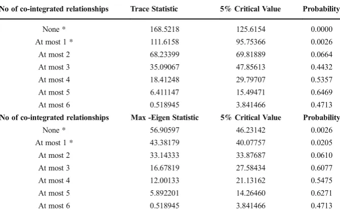
Before testing for the co-integration rank, the appropriate lag length for the under-lying empirical VECM model is identified based on the Lagrangian multiplier (LM) test for serial correlation of the residuals.16The Johansen (1995) procedures were then applied to test for the co-integration rank. From the Trace test and the Max-Eigen test, two co-integrating vectors were employed. Table 2 presents the results of the co-integration rank test.

The rank of the Π-matrix was found to be r= 2 implying that statistically a discrimination among two conditionally independent stationary relations is pos-sible. The two unrestricted co-integration relations are uniquely determined but the question remains on whether they are meaningful for economic interpreta-tion. Consequently, Johansen and Juselius (1994) identifying restrictions were imposed to distinguish among the vectors and ensure the uniqueness of the

13

Data are collected from Datastream.

14

Data from the United States are used as a proxy for foreign variables and data from the UK as proxies for domestic variables.

15_{For robustness purposes we have also performed the Kwiatkowski, Phillips, Schmidt, and Shin (KPSS) test}

with stationarity under the null. The KPSS also suggests that the variables are integrated of order one i.e. I(1).

16

coefficients. By taking a linear combination of the unrestricted β vectors, it is always possible to impose r−1 just identifying restrictions and one normaliza-tion on each vector without changing the likelihood funcnormaliza-tion. Although the normalization process can be done arbitrarily it is generally accepted practice to normalize on a variable that is representative of a particular economic relation-ship. Since the purpose of the paper is to identify a possible long-run deter-mination of the real exchange rate, the co-intergrated vectors are normalized with respect to the real exchange rate. Additional restrictions (as implied by the Table 1 Augmented Dickey-Fuller test for a unit root

Variable Test in levels Test in differences

No Trend Trend No Trend Trend

lqt −3.29(0)† −3.50(0)† −9.27(1)* −9.22(1)*

lMt −2.61(0) −0.53(0) −8.88(0)* −9.24(0)*

lM*

t 1.23(1) −0.61(1) −4.69(0)* −4.97(0)*

lrt −0.74(1) −2.59(1) −5.96(0)* −5.96(0)*

lr*

t −0.99(1) −2.27(1) −7.88(0)* −7.83(0)*

lPS

t −1.98(0) −2.28(0) −10.67(0)* −10,70(0)*

lPFSt ;* −1.69(0) −2.08(0) −11.00(0)* −11.01(0)*

Note: Entries in parenthesis indicate the lag length based on SIC maxlag = 12

†indicates that the test is significant at 1% and 5% (*) indicates that the test is significant at all critical values.

Table 2 Results of co-integration test

No of co-integrated relationships Trace Statistic 5% Critical Value Probability

None * 168.5218 125.6154 0.0000

At most 1 * 111.6158 95.75366 0.0026

At most 2 68.23399 69.81889 0.0664

At most 3 35.09067 47.85613 0.4432

At most 4 18.41248 29.79707 0.5357

At most 5 6.411147 15.49471 0.6469

At most 6 0.518945 3.841466 0.4713

No of co-integrated relationships Max -Eigen Statistic 5% Critical Value Probability

None * 56.90597 46.23142 0.0026

At most 1 * 43.38179 40.07757 0.0205

At most 2 33.14333 33.87687 0.0610

At most 3 16.67819 27.58434 0.6077

At most 4 12.00133 21.13162 0.5475

At most 5 5.892201 14.26460 0.6271

At most 6 0.518945 3.841466 0.4713

economic model) are also imposed, namely that δ2= −δ1,δ3=δ1, δ4= −δ3 and δ6= −δ5.

In addition, all foreign variables, i.e.lM*

t,lr*t and lP FS;*

t are treated as weakly

exogenous variables, thus long run forcing in the co-integrating space. This can be justified under the assumption that the UK is a small open economy, as such domestic policy decisions or more generally domestic economic activity do not have a significant impact on the evolution of foreign variables. Consequently, treating all variables as jointly endogenously determined would lead to inappropriate inference. The restrictions identify all co-integrating vectors, and according to Theorem 1 of Johansen and Juselius (1994) the rank condition is satisfied.

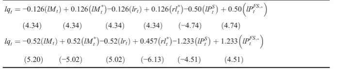
Table3 reports the constrained coefficients from the long-run co-integrating rela-tionships normalized with respect tolqt17. In both vectors all variables are statistically

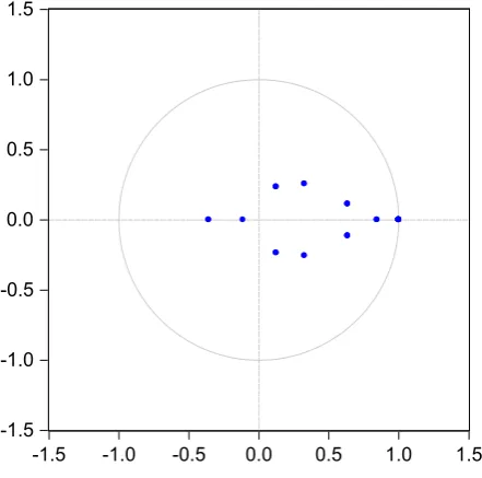
significant and correctly signed in accordance with the predictions of the theoretical model. The results reveal that the stock market variables are highly associated with the real exchange rate in the long run as compared with bond returns and money balances. Fig.1presents the two co-integrating graphs showing evidence of stationarity. From both co-integrating vectors it can be estimated that the value for the parameterεlies between 0.5 and 1 as assumed in the theoretical set up. To test the stability of the VECM model the inverse roots of the characteristic AR polynomial are reported in Fig.

2. The analysis confirms that the VECM is stable since the inverted roots of the model lie inside the unit circle. Having established that the VECM is stable, the identified long-run co-integrating relationships, normalized on the real exchange rate, can be interpreted.

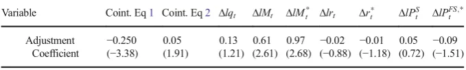
Table 4 reports the adjustment coefficients on the dynamics of the adjust-ment process towards equilibrium. With an adjustadjust-ment coefficient of −0.25 in the first co-integrating equation there is evidence that the real exchange rate tends to stabilize itself by 25% per quarter. The adjustment coefficients of all other variables apart from the money balances turn out to be insignificant. Additional tests related to the statistical viability of the results indicate that there is no serial correlation of the residuals, no evidence of heteroscedasticity and that the residuals are normally distributed18.

Table 3 Long-Run Co-integrating Relationship (constrained coefficients)

lqt¼−0:126ðlMtÞ þ0:126lM*t

−0:126ð Þ þlrt 0:126rl*t

−0:50lPS_t þ0:50 lPFSt ;*

4:34

ð Þ ð4:34Þ ð4:34Þ ð4:34Þ ð−4:74Þ ð4:74Þ

lqt¼−0:52ðlMtÞ þ0:52lM*t

−0:52ð Þ þlrt 0:457rl*t

−1:233lPS_t þ1:233 lPFSt ;*

5:20

ð Þ ð−5:02Þ ð5:02Þ ð−6:13Þ ð−4:51Þ ð4:51Þ

Note:t statistics in parentheses

All constraint coefficient are statistically significant at 5% level and correctly signed in accordance with the predictions of the model

17

The two co-integrating vectors are linearly independent.

18

4 Economic Interpretation of Results

The model predicts that an expansionary monetary policy in the UK in a form of an increase in the nominal money supply will result in a real appreciation of the long run real exchange rate i.e.δ1< 0. The estimated coefficient for the domestic (UK) nominal

money supplylMt, as depicted in Table3is negative supporting the prediction of the

model. The prediction of the model regarding the increase in the domestic money supply is because in the long run the price level will accommodate the increase in the nominal money supply (given that money neutrality holds) but the nominal exchange rate depreciates to a lesser extent as PPP does not hold in the long run. In a similar manner, the model predicts real exchange rate depreciation after an increase in the foreign (USA) nominal money supplylM*_t (δ2> 0). The coefficient for the foreign -.3

-.2 -.1 .0 .1 .2 .3 .4

90 92 94 96 98 00 02 04 06 08 10 12 14

Cointegrating relation 1

-0.8 -0.4 0.0 0.4 0.8 1.2

90 92 94 96 98 00 02 04 06 08 10 12 14

Cointegrating relation 2

Fig. 1 The graphs of the co-integration relations

-1.5 -1.0 -0.5 0.0 0.5 1.0 1.5

-1.5 -1.0 -0.5 0.0 0.5 1.0 1.5

money supply has a positive sign, providing further evidence in favour of the theoret-ical model.

The model predicts that an increase in the real bond returnlrtresults in a long run

real exchange rate appreciation i.e.δ3< 0. The estimated coefficient in Table3forlrtis

also negative supporting the prediction of the model. An explanation is that an increase in the real bond return may increase the demand of domestic currency, which induces both a nominal and real appreciation of the domestic currency in the long run. Likewise, the model predicts a real depreciation after an increase in the real foreign bond returnslr*

t i.e.δ4> 0. This prediction is also borne out in our empirical test of the

model.

Finally, the model predicts that an increase in the domestic (UK) share price index will lead into a real appreciation of the long run real exchange rate i.e.δ5<

0, which is confirmed in our results. The relationship between stock prices and exchanges rates that has been examined in the literature depends on the relative strengths of the income and substitution effects. A possible explanation for the appreciation of the real exchange rate (also predicted by the theoretical model) could be associated with a domination of the income effect and the subsequent increase in the demand for real money balances. The subsequent increase in the interest rate (in order to satisfy equilibrium in the money market) induces capital inflows and results in both a nominal and a real appreciation. Similarly, an increase in the foreign (USA) stock market index leads to a real depreciation of the exchange rate i.e.δ6> 0, which is also confirmed by our results.

5 Concluding Remarks

This paper contributes towards the theoretical determination of the real ex-change rate by constructing an intertemporal optimization model, which incor-porates investment in an array of assets such as domestic and foreign bonds, domestic and foreign stocks, and domestic and foreign real money balances. Such an approach to the determination of the real exchange rate in the long-run has been neglected in the current literature, which is heavily based on the BEER and FEER models as well as on other extensions of the basic balance of payment equilibrium approach.

Table 4 Adjustment coefficients

Variable Coint. Eq1 Coint. Eq2 Δlqt ΔlMt ΔlMt* Δlrt Δr*t ΔlPSt ΔlP FS;* t

Adjustment Coefficient

−0.250 (−3.38)

0.05 (1.91)

0.13 (1.21)

0.61 (2.61)

0.97 (2.68)

−0.02

(−0.88)

−0.01

(−1.18) 0.05 (0.72)

−0.09

(−1.51)

The basic predictions of the model are borne out empirically suggesting that asset prices and returns play an important role in the determination of the long run real exchange rate and its evolution. The model suggests that an increase in the domestic money supply, an increase in the domestic real bond returns and an increase in the domestic economy’s stock market will lead into a real exchange rate appreciation in the long run while increases in the corresponding foreign variables will lead to a real exchange rate depreciation. Given the importance of the role of the real exchange rate for policy makers and the functioning of open economies our contribution provides an alternative frame-work to much of the existing literature.

Our results suggest that future research would benefit from incorporating a range of asset prices when considering the equilibrium real exchange rate. There is also scope for future research to consider how mispricing of financial assets may also have feedback effects on the real exchange rate and hence on the real economy. It would also be interesting to compare the results of our model with the alternative methods of modelling the real exchange rate to see the extent of any quantitative and qualitative differences.

Acknowledgements We are extremely grateful to George Chortareas, Jose Olmo, Gabriel Montes-Rojas, Sushanta Mallick, William Pouliot, Roy Bailey, Keith Cuthbertson and Joscha Beckmann and the participants at the European Economics and Finance Society 15th Annual Conference in Amsterdam for many useful comments and suggestions. We are also particularly heavily indebted to two anonymous referees for their extensive comments that led to significant improvements in the paper. Any errors and omissions remain those of the authors.

APPENDIX I

The derivation of the real exchange rate equation

Substituting equation (26) into equation (27) and equation (28) into equation (25) in the text the following equation is derived:

mt m* t

¼ α−σ

ε Ch t

σ ε_q

t

ð Þσθεð Þ_Tt −σθε_Xε1 ð1−αÞ−σε _Cf t

σ ε

qt

ð Þσθ−1

ε

½ _X1

εð Þmt

1−ϵ

ð Þ

ϵ ₁− P

S;* tþ1þd

* t

PS;* t

−1

−1

ε

( )1−ε

ε iD

t

1þiD t h i−1

ε

1−α

ð Þ−σ

ε _Cf t

σ ε

qt

ð Þσθ−1

ε

½ _X1

ε α−σε Ch t

σ ε_q

t

ð Þσθεð Þ_Tt −σθε_X1ε m* t

1−ε

ε ₁₋ PStþ1þdt

PS t

−1

−1

ε

( )1−ϵ

ϵ iF

t

1þiF t h i−1

ε

which simplifies to:

mt

m* t

¼₁₋α_α−

σ ε Cht

Ctf

!σ

ε

qt ð Þ½ σθε _q

t

ð Þ−σθ−1

ε

½ _{ð Þst} −σθ ε 1−α

α

−σ

εð1−εεÞ

½ _Cf

t

Ch t

!σ

εð1−εεÞ

½

qt ð Þ−1−σθ

ε

½ 1−ε

ε

½ _q

t ð Þ−½ σθε½ 1−εε _s

whereΩ¼

mt

ð Þ1−∈∈

1−_εε

1− P

S;* tþ1þd*t

PS_t;*

−1

−1

ε

( )1−ε

ε

iD_t

1þiD_t

h i−1

ε

m* t

ð Þ1−∈_∈

1−_εε

1− PStþ1þdt PS_t

−1

−1

ε

( )1−∈_∈

i F_t

1þi F_t

h i−1

ε

mt

m*

t

¼ Cht

Ctf

!−σ

ε

Tt

ð Þσθε C

h t

Ctf

!σ

ε

q_t

ð Þσθε−½ σθε−1ð Þ_Tt −σθε _q

t

ð Þ−1−σθ ε

½ 1−ε ε

½ _q

t

ð Þ−½ σθε ½ 1−εε Ω

mt

m*

t

¼ð Þq_t 2εε−21 :Ω ð₃₁Þ

Dividing equation (6) with equation (8) yields that:_P1S

t ¼

1þiD t

PS

tþ1þdt, which implies that:

PS_t− PS_tþ1þdt

¼− PS_tþ1þdt

iD_t

1þiD t

ð32Þ

In a similar manner dividing equation (7) with equation (9) implies that:

P_tS;*− P_tS_þ;*₁þd*_t

h i

¼− PS_tþ;*₁þd*_t

h i _iF

t

1þiF t

ð33Þ

Using Equations (32) and (33) and dividing equation (8) with equation (9) implies

that PSt

PSt;*¼

etþ1

et :

PS tþ1þdt

PS_tþ;*₁þd* t

, Equation (31) becomes

mt m* t

¼ð Þqt

2ε−1 ε2 _m

t

ð Þ ð1−ϵϵ2Þ2

m*t −ð1−ϵÞ2

ϵ2

PStþ;*1þd

* t h i− 1−ε

ε2

i*t − 1−ε

ε2

et−

1−ε ε2 _PS

t

− 1−ε ε2

etþ1 1−ε

ε2 _PS;*

t

1−ε ε2

PS_tþ1þdt

1−ε

ε2 _ih

t

1−ε ε2

ih_t

−1

ε

½ _i* t

1

ε

½

Where ih t

¼ iD t 1þiD

t

h i

and i* t

¼ iF t 1þiF

t

h i

Taking logs of all variables we obtain equation (34):19

lqt¼δ1ðlMtÞ þδ2 lM*t

þδ3ð Þ þlrt δ4 lr*t

þδ5 lPSt

þδ6 lPFSt ;*

_ð

34Þ Where:δ1¼− 2₁ε₋−_ε1

;δ2¼ 2₁ε₋−_ε1

;δ3¼− 2₁ε₋−_ε1

;δ4¼ 2₁ε₋−_ε1

;δ5¼− ₁₋ε_ε ;δ6 ¼ ₁₋ε_ε

Equation (34) corresponds to equation (29) in the text.

19_{Following the fact that} PS t

PSt;*¼

etþ1

et:

PS tþ1þdt

PStþ;*1þd * t

and assuming that capital and consumption are homogeneous

APPENDIX II

Variable Explanation

Ct Real consumption of a composite bundle of goods

mt¼MPtt Domestic real money balances, withMtdomestic nominal money balances andPtthe consumer

price index of the composite good consumed domestically. m*

t ¼ M*

t

P* t

Foreign real money balances, withM*

tforeign nominal money balances andP*t the consumer price index of the composite good consumed in the foreign economy.

yt Real income

et Nominal exchange rate (amount of foreign currency per unit of domestic currency)

BD

t Amount of domestic currency invested in domestic bonds BF

t Amount of foreign currency invested in foreign bonds iD

t Nominal rate of return on domestic bonds iF

t Nominal rate of return on foreign bonds St Number of domestic shares purchased

S*

t Number of foreign shares purchased PS

t Domestic share price PSt;* Foreign share price

dt Value of domestic dividend earned

d*_t Value of foreign dividend earned Uc,t Marginal utility from consumption

UM_P;t Marginal utility from domestic real money balances

UM * P*;t

Marginal utility from foreign real money balances Cht Consumption of domestically produced goods Ctf Domestic consumption of foreign imported goods Ph

t The price index of domestically produced goods

Ptf Price index of goods produced in the foreign economy (expressed in units of domestic currency) Pf∗ _{Price index of goods produced in the foreign economy}

Ph*

Foreign currency equivalent of the price index of domestically produced goods Tt Terms of trade

qt Real exchange rate–a rise represents a real depreciation a fall represents a real appreciation

ih t

iD t

1þiD t

h i

i* t

iF t

1þiF t

h i

lPFS_t ;* lPS_t;*−let(ldenotes log) lrt liht−lPt(ldenotes log) lr*

t li*t−lP*t (ldenotes log)

Reference

Bacchetta P, van Wincoop E (2004) A scapegoat model of exchange rate determination. Am Econ Rev 96: 552–576

Bacchetta P, van Wincoop E (2013) On the unstable relationship between exchange rates and macroeconomic fundamentals. J Int Econ 91:18–26

Clark, P. and MacDonald, R. (1998) Exchange rates and economic fundamentals: A methodological compar-ison of BEERs and FEER’s,IMF Working PaperWP98/67

Dellas H, Tavals G (2013) Exchange rate regimes and asset prices. J Int Money Financ 38:85–94

Driver, R.L. and Westaway, P.F. (2004) Concepts of equilibrium exchange rates,Bank of England, Working Paper No. 248

Fratzscher M et al (2015) The scapegoat theory of exchange rates: The first tests. J Monet Econ 70:1–21 Galí J, Monacelli T (2004) Monetary policy and exchange rate volatility in a small open economy. Rev Econ

Stud 72:704–734

Johansen S (1988) Statistical analysis in co-integrated vectors. J Econ Dyn Control 12:231–254

Johansen S (1991) Estimation and hypothesis testing of co-integration vectors in gaussian vector autoregressive models. Econometrica 52:389–402

Johansen S, Juselius K (1994) Identification of the long-run and short-run structure: an application to the ISLM model. J Econ 63:7–36

Johansen S (1995) Likelihood–based inference in cointegrated vector autoregressive models, Advanced texts in econometrics. Oxford University Press, Oxford

Juselius K (2006) The cointegrated VAR model: Methodology and applications. Oxford University Press, Oxford

Kia A (2006) Deficits, Debt financing, monetary policy and inflation in developing countries: internal or external factors? Evidence from Iran. J Asian Econ 17:879–903

MacDonald, R. (2000) Concepts to calculate equilibrium exchange rates: An overview,Deutsche Bundesbank No. 2000, 03

Rogoff K (1996) The purchasing power parity puzzle. J Econ Lit 34:647–668

Walsh CE (2003) Monetary theory and policy. Massachusetts Institute of Technology, Massachusetts Williamson J (1994) Estimates of FEERs. In: Williamson J (ed) Estimating equilibrium exchange rates.