Gaussian Process Model
Ravi Kumar Pandit, David Infield
University of Strathclyde, Glasgow, Scotland, G1 1XQ, UK
[email protected] [email protected]
ABSTRACT
Loss of wind turbine power production identified through performance assessment is a useful tool for effective condition monitoring of a wind turbine. Power curves describe the nonlinear relationship between power generation and hub height wind speed and play a significant role in analyzing the performance of a turbine.
Performance assessment using nonparametric models is gaining popularity. A Gaussian Process is a nonlinear, non-parametric probabilistic approach widely used for fitting models and forecasting applications due to its flexibility and mathematical simplicity. Its applications extended to both classification and regression related problems. Despite promising results, Gaussian Process application in wind turbine condition monitoring is limited.
In this paper, a model based on a Gaussian Process developed for assessing the performance of a turbine. Here, a reference power curve using SCADA datasets from a healthy turbine is developed using a Gaussian Process and then was compared with a power curve from an unhealthy turbine. Error due to yaw misalignment is a standard issue with a wind turbine, which causes underperformance. Hence it is used as case study to test and validate the algorithm effectiveness. 1.INTRODUCTIONS
Use of wind energy to meet energy needs is considered as a vital alternative option to deal with existing global fossil fuel crisis and climate change. Wind energy is one of the fastest growing sources of power production in the world today, but still considered to be expensive, hence there is a constant need to reduce the cost of operating and maintaining them, i.e., Operation and maintenance (O&M) cost, especially offshore, (Hyers, R. W et al.2006). Active condition monitoring can help ensure a low cost of energy (COE),
increase life expectancy and improve the efficiency of a turbine. Condition monitoring is a widely used tool for early detection of failures and or faults to minimize the downtime, maximize the productivity and prevent turbines from catastrophic damage.
Readily available Supervisory control and data acquisition (SCADA) datasets obtained from operational wind turbines are a cost-effective condition monitoring approach since these data sets are freely available and contain vital information about the wind turbines (Zaher, A et al.2009). Proper understanding of these SCADA datasets is useful for constructing robust models for condition monitoring and thus helpful in reducing the operation and maintenance (O&M) costs, which could reach up to 1/3rd Of the total project cost,
especially for offshore wind turbines where O&M costs are high, (Martin, R et al. 2016).
Power curves are significant for developing robust models for condition monitoring purposes; they record the power generation of a turbine at different hub height wind speeds. SCADA datasets obtained from healthy turbine were used to fit bivariate probability distribution functions, illustrating the power curve of existing turbines, which is useful for identifying the anomalous or abnormal behavior, (M. Lydia et al.2014). Both parametric and nonparametric models have used for fitting the power curve for wind turbine condition monitoring. Polynomial regression (a parametric model) gives a smooth power curve fitting, however, as suggested in (S. Shokrzadeh et al.2014), it is very much responsive to anomalies within the observations and requires the high degree polynomial regression model to give suitable and accurate fitting to the measured data sets. Also, it is worth noting that parametric models are mostly based on fundamental equations of power available in the wind and do not represent the precise characteristics of actual turbines, (Thapar V et al.2011) hence nonparametric models come into play and are described in next paragraph.
_____________________
Non-parametric models are in the wind turbine area since they are relatively more accurate than parametric models because they do not impose any pre-specified model formulations, see Ref. (S. Shokrzadeh et al.2014), Neural networks (Leszek Romański et al.2017), fuzzy logic methods (Lorenzo Dambrosio.2017), kNN (Raik Becker et al.2017), cubic spline regression (T. Ouyanga et al.2017), Non-linear state estimation technique (NSET) (Y. Wang & D. Infield.2013), random forest (Y. Si et al.2017), Gaussian Process (GP) (R. K. Pandit & D. Infield.2017), are widely used non-parametric models for wind turbines, for further details about these nonparametric methods see (S. Shokrzadeh et al.2014) and (Thapar V et al.2011).
A Gaussian Process (GP) is a nonparametric, nonlinear machine learning approach increasingly used in recent times for wind turbine modeling due to its flexibility and simplicity in constructing the nonlinear models. In contrast, Ref (Neal, R. M.,1994), Artificial Neural Networks (ANN), a nonparametric model constructed which entirely depends on training parameters and the input function for the convergence makes the ANN model complex, while a Gaussian Process model is easy to understand and uses few assumptions for developing a useful GP model. Also, GP models can be optimized precisely for a given value of their hyper-parameters: the weight decay and the spread of a Gaussian kernel, Ref. (C. E. Rasmussen & C. K. I. Williams.2006). These strengths make GPs an ideal choice for solving problems related to fitting, forecasting and anomaly detection related to operation and maintenance (O&M), rightly described in (Xueru Wang et al.2014) and (Niya Chen et al.2013). GPs are also useful for constructing a preventive model for early detection of faults or anomalies which will be helpful in preventing the turbine experience catastrophic damage. GP algorithms allow continuous monitoring of turbine health by constructing automated failure detection algorithms; this improves reliability and reduces the O&M cost by eliminating unnecessary scheduled maintenance.
This paper introduces the application of a Gaussian Process in assessing the performance of wind turbine based on power curves. Yaw misalignment affects the performance of a wind turbine. Hence, this is used here as a test case to validate the proposed GP model effectiveness. The ability to highlight performance deviations and GP model effectiveness investigated by use of real measurements available in the form of SCADA datasets obtained from the operational wind turbine (Kim K et al.2011). The strength and weakness of GP models will be assessed and summarised at the end of the paper.
2.SCADADATADESCRIPTION,IMPORTANCE ANDPRE-PROCESSING
Supervisory control and data acquisition (SCADA) system
monitoring and or operation and maintenances (O&M). Using SCADA based condition monitoring considered as cost-effective (since this information is freely available without extra cost) unlike existing condition monitoring approaches, e.g., Vibration analysis and oil debris detection are expensive, which increases the overall cost of O&M, (Kusiak A & Zhang Z. 2010) and (P. Dao et al.2018). SCADA datasets play a vital role in constructing a preventive model for early fault or anomaly detections.
SCADA data comes with operational and technical details of a turbine component and typically 10 minutes’ average data used in wind industries for fault diagnosis and prognosis activities, (Zaher AS et al.2007). Despite such advantageous; SCADA datasets are not free from measurement error which recorded in SCADA datasets due to sensor malfunction and or failures and if such error allowed in the model analysis then the result would be inaccurate. Hence, it is desirable to minimize these errors before making further analysis. Criteria for examples; timestamp mismatches, out of range values, negative power values, and turbine power curtailment being used as per Ref. (M. Schlechngen & I. F. Santos.2011) to remove deceptive data and being used to model measured power curve in which air density correction applied as per IEC standards 61400-12-1, (IEC 61400-12-1. 2006) described in the next section. The 2.3 MW Siemens turbines (located in Scotland) SCADA datasets of 2009 a year considered in this paper for constructing a reference fitted GP power curve described in section 5.
3.POWERCURVEMODELINGFOR PERFORMANCEASSESSMENTOFAWIND
TURBINE
Power curve widely used to assess, monitor and analyze the performance of a wind turbine with the help of the operational data of wind power plant which is available in the form of SCADA data points. Due to the continuous evolution of turbine rotor sizes, the importance of the SCADA system and a met mast became more dominating to evaluate the turbine performance, and with the use of up-to-date technology (e.g., Remote sensing), a better understanding of turbine performance can be explained.
IEC standards 61400-12-1 suggests the ‘methods of bins’ for constructing the measured power curve of wind turbines which is useful for annual energy estimations. Though it is worth to note that the fast wind fluctuations in 10 min averaging datasets may not include IEC binning methods, and hence particular attention needs to be paid, (IEC 61400-12-1. 2006).
Power curve used to describe the relationship between the power output of a turbine and the wind speed at the turbine site and mathematically expressed as,
where ρ is Air density (𝑘𝑔 𝑚⁄ 3), A is swept area (𝑚2) , 𝐶 𝑝 is the power coefficient of the wind turbine and 𝑣 is the hub wind speed (𝑚 𝑠𝑒𝑐⁄ ). The equation (1) report the simple relationship with limited precision due to the complexity and the influences of these parameters on turbine productivity. The power coefficient is a strong function of the tip speed ratio and pitch angle (β). Although, WTs also depends on flow conditions for examples; terrain, wind shear, turbulence intensity and air density, Ref. (Vaishali Sohoni et al.2016) and needs to be investigated its impact on Gaussian Process model and reserved for a future task.
IEC binned power curve influenced by ambient temperature, humidity, and pressure and hence affects the power production of a wind turbine. Out of these parameters, the temperature has the highest contribution to air density, and therefore IEC recommend air density correction prior making further analysis for accurate power curve modeling. The SCADA datasets used in this paper are from a pitch-regulated wind turbine and hence as per IEC standard, air density correction being applied using equations (2) and (3) where corrected wind speed 𝑉𝐶 is calculated as follows,
ρ = 1.225 [
288.15T
] [
B
1013.3
]
(2)and,
V
C= V
M[
ρ1.225
]
1 3
[image:3.612.75.264.506.663.2](3) where, 𝑉𝐶 and 𝑉𝑀 are the corrected and measured wind speed in m/sec and the corrected air density is calculated by equation (2) where B is atmospheric pressure in mbar and T the temperature in Kelvin in which 10 minute average values obtained from SCADA data are used. Using above equations, a corrected and filtered (using section 2) power curve being constructed and is shown in figure 1 and these datasets would be used in upcoming sections for developing GP algorithm related to performance assessments.
Figure 1. Filtered and corrected power curve
4.YAWMISALIGNMENT- A CASESTUDY
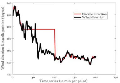
A significant loss of wind turbine power can be due to yaw misalignment. Ref. (Avent lidar technology. 2013) suggests that an average of misalignment causes an estimated 2 % reduction in annual energy production (AEP) with roughly a loss of 2 - 3% for of average yaw error. Yaw error not only reduces the power production but also increases component loads, for instance (J. G. Schepers.2007) suggested that yaw misalignment had effects on blade root and shaft loads. Another article, (K. Boorsma.2012), found that for a 2.5 MW wind turbine that edgewise fatigue equivalent loads increased with an increase in yaw error. Theoretically, power output is reduced by the cube of the yaw misalignment error, though Ref. (M. Spencer et al.2013) and (K. A. Kragh & P. Fleming. 2012) suggests a better relationship could be cosine-squared instead of cosine-cubed, as validated by empirical data. Principally, yaw position regulated in response to the wind direction change to extract maximum power productions from a wind turbine. Various machine learning approaches have been developed for wind direction prediction, for example, in Ref. (Song, D et al.2017) Two models proposed, namely; a univariate auto-regressive integrated moving average (ARIMA) model and a hybrid model that merges the ARIMA model into the Kalman filter (KF). The results suggest that the hybrid model performs better in terms of various performance indicators.
Active yaw alignment increases performance and power production of a wind turbine. For example, (PMO Gebraad et al.2016), applying a game-theoretic optimization approach to yaw misalignment, increases the power production of a simulated wind farm. Wind tunnel testing of two turbines has evaluated a Bayesian optimization model, using yaw and blade pitch as inputs as described in (Jinkyoo Park & Kincho H Law.2015). Ref (PMO Gebraad et al.2016) suggest that combined optimization of yaw control and layout can reduce the cost of energy from wind farms. In short, yaw misalignment impacts on power output and loads.
Based on the above discussion, yaw error and or misalignment is considered to provide an appropriate case study for validating the effectiveness of performance assessment algorithms of a GP model. SCADA datasets from an unhealthy turbine over the time period from 13th April
2009 to 18th April 2009 has been selected since the yaw
Figure 2. Absolute yaw error in time series
Figure 3. yaw misalignment via wind direction and nacelle direction in time series
5.GAUSSIANPROCESSMODELSFORWIND TURBINEPERFORMANCEASSESSMENTS
A Gaussian process (GP) is a stochastic, nonlinear and nonparametric model whose distribution function is the joint distribution of a collection of random variables and widely suitable for classification and regression problems, (C. E. Rasmussen & C. K. I. Williams.2006) and (Ping Li & Songcan Chen.2016). GP is a machine learning algorithm using a lazy learning approach and uses the measure of similarity between the points (via covariance functions) to fit and or estimate the future value from a training dataset. In Bayesian inference, a GP can be used as a prior probability distribution over the functions, (Rasmussen and Williams 2006). Multivariate Gaussian distributions control the manipulation of the GP model when a finite number of data points observed. A Gaussian Process 𝑓(𝑥) is fully defined by mean function 𝑚(𝑥) and covariance function
𝐾(𝑥, 𝑥
′)
as
follows,𝑓(𝑥) ~ 𝐺𝑃(𝑚(𝑥) , 𝐾(𝑥, 𝑥
′))
(4) Here, mean functions 𝑚(𝑥) is an 𝑛 × 1 vector and 𝐾(𝑥, 𝑥′) is an 𝑛 × 𝑛 matrix as described below,𝑚(𝑥)
𝑘(𝑥, 𝑥) 𝑘(𝑥, 𝑥
′)
The covariance functions define the correlations between different points, i.e., calculates the likeness between these points and considered to be sole of any GP models and decided factor for judging the GP models accuracy. There are varieties of covariance functions (or kernel) available and well described in Ref. (C. E. Rasmussen & C. K. I. Williams.2006). For this paper, a squared exponential covariance function used since it has been shown to work well with wind turbine power curve estimation. For any finite collection of input {𝑥1, 𝑥2, … . . , 𝑥𝑛}, squared exponential covariance functions (SECov) mathematically defined as below,
𝑘
𝑆𝐸(𝑥, 𝑥
′) = 𝜎
𝑓2exp (−
(𝑥−𝑥 ′)22𝑙2
)
(5) SCADA data of the wind turbine comes with measurement errors, so to compensate these error effects, it is desirable to add a noise term to the covariance function to minimize its impact and improve the accuracy of the GP model. Hence equation (5) modified to be:
𝑘
𝑆𝐸(𝑥, 𝑥
′) = 𝜎
𝑓2exp (−
(𝑥−𝑥 ′)22𝑙2
) + 𝜎
𝑛2
𝛿(𝑥, 𝑥′)
(6) where 𝜎𝑓2, 𝜎𝑛2 and𝑙 are known as the hyper-parameters. 𝜎𝑓2 signifies the signal variance and 𝑙 is a characteristic length scale which describes how quickly the covariance decreases with the distance between points. σ𝑛 is the standard deviation of the noise fluctuation and gives information about model uncertainty. 𝛿 is the Kronecker delta. Effective Optimization of these hyper parameters govern GP models behaviour and accuracy. The optimization of these hyper parameter described in next paragraph.
To construct a GP power curve, the first step is to estimate the mean value and variance for the given training data set A of n observations, 𝐴 = {(𝑈𝑖, 𝑃𝑖), 𝑖 = 1, … … , 𝑁}, where 𝑈𝑖 and 𝑃𝑖 are the wind speed and power values respectively. For our application, consider the observed values 𝑦𝑖 are modeled as the sum of true function 𝑓(𝑥𝑖) plus added Gaussian noise as follows:
𝑦
𝑖= 𝑓(𝑥
𝑖) + 𝜖
𝑖 (7) The above equation is theoretically used to define the underlying function of the data modeled where 𝑥 are values from the training datasets and 𝜖 is Gaussian white noise of variance 𝜎𝑛2 such that, 𝜖 = 𝑁(0, 𝜎𝑛2). [image:4.612.77.268.241.373.2]which {𝑃∗ , 𝑈∗} are the future power and wind speed values. 𝑃𝑡𝑟, 𝑈𝑡𝑟 are the training SCADA datasets of power and wind speed respectively.
The squared exponential covariance function depends on hyper-parameters which needed be optimised before the posterior distribution of 𝑃∗ is calculated in order to ensure GP model accuracy. Maximization of the log marginal likelihood has been used here to optimize the hyper parameters (𝜎𝑓2 , 𝜎𝑛2and𝑙), (see for example Rasmussen and Williams 2006), through the application of the following equation:
𝑙𝑜𝑔(𝑝(𝑃
𝑡𝑟|𝑈
𝑡𝑟)) = −0.5𝑃
𝑡𝑟𝑇𝐾
−1𝑃
𝑡𝑟−
0.5𝑙𝑜𝑔(|𝐾|) − 05𝑛𝑙𝑜𝑔(2𝜋)
(8)
A quasi-Newton optimization method was used to optimize the hyper-parameters through the likelihood function (equation 8) in simple ML-II fashion, (C. E. Rasmussen & C. K. I. Williams.2006) and (Jie Chen & Nannan Cao.2013). This optimization approximates the Hessian and uses a trust-region method with a dense, symmetric rank-1-based(SR1). After optimization, the prediction of the distribution of 𝑃∗ for a given 𝑈∗ is simple and straightforward. The predicted distribution of 𝑃∗, p(𝑃∗|𝑈∗, 𝑈𝑡𝑟, 𝑃𝑡𝑟) follows a Gaussian distribution with mean and variance expressed by following equations,
𝑚(𝑃
∗) = 𝑘
∗𝑇𝐾
−1𝑃
𝑡𝑟 (9)𝜎
2(𝑃
∗) = 𝑘
∗∗− 𝑘
∗𝑇𝐾
−1𝑘
∗+ 𝜎
𝑛2 (10) where,𝑘∗= [𝑘(𝑈∗, 𝑈1)𝑘(𝑈∗, 𝑈2)𝑘(𝑈∗, 𝑈3) … … … 𝑘(𝑈∗, 𝑈𝑛)]𝑇 are covariance values between test and training data points in the form of column vector and 𝑘∗∗= 𝑘(𝑈∗, 𝑈∗) is the auto covariance function of the testing data points. The obtained 𝜎2 is the variance of the predicted function and is used to estimate the confidence intervals (chosen to be 95% ) of the GP power curve model using equation (11).
𝐶𝐼
𝑛= 𝑚
𝑛± 2𝜎
𝑛 (11)Despite having advantages especially in dealing with nonlinear models, GP accuracy suffers when dealing with a large number of data points due to the well-known cubic inversion issue. Some of the proposednon
-parametricmethods, for example (J.Hartikainen et al. 2010), (S. Sarkka et al.2013) and (Jie Chen & Nannan Cao.2013) aim to solve this issue but these methods need high processing power and computational cost. Finding an appropriate balance between computational cost and processing power is the key to effective GP modeling for anomaly detection for wind turbine condition monitoring. Using the filtered and air density corrected power curve of figure 1, a GP algorithm for power curve estimation was developed and realized in MATLAB, with the result shown in figure 4. The GP power estimation closely matches the
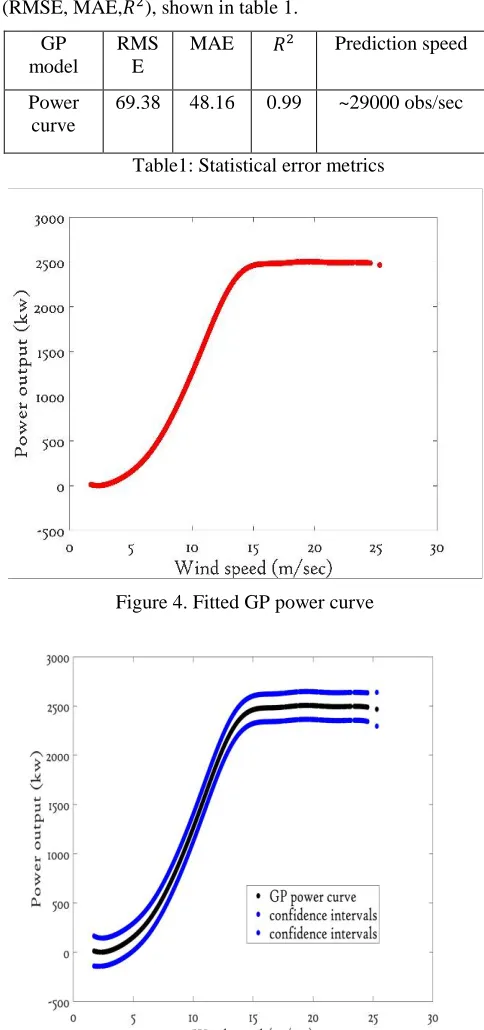
measured power, as shown in figure 6 where power has been plotted as a time series (of 10-minute points). The accuracy of the model is confirmed by the statistical error metrics (RMSE, MAE,𝑅2), shown in table 1.
GP model
RMS E
MAE 𝑅2 Prediction speed
Power curve
69.38 48.16 0.99 ~29000 obs/sec
[image:5.612.314.556.109.624.2]Table1: Statistical error metrics
[image:5.612.325.536.382.626.2]Figure 4. Fitted GP power curve
Figure 6. Fitted GP power comparison with measured power in time series
The unique feature regarding GP estimation is the provision of not only an estimate for that point in question but also information about uncertainty via its confidence intervals (CIs), which plays a vital role in using a GP model for early fault detection. These GP confidence intervals provide knowledge about the uncertainty surrounding an estimation, but is itself a model-based estimate, see for example (Neyman, J. 1937). In (Alain Bensoussan et al. 2014), confidence intervals for annual wind power productions defined whereas in (Breno Menezes.2014), confidence intervals for reservoir computing’s wind power generation applied. The datasets recorded in the form of SCADA datasets are considered as noisy hence GP estimates of confidence do not include this, but the model does separately estimate the magnitude of the associated uncertainty. For a practical GP model, it is desirable to modify the confidence intervals to minimize the noise impacts, (Andrew McHutchon & Carl Edward Rasmussen.2011). Hence the fitted GP power curve with adjusted confidence intervals is plotted in figure 5. It is worth noting that in figure 5, the confidence intervals (CIs) represent the pointwise mean plus and minus two times the standard deviation for given input value (corresponding to the 95% confidence region which represents the significance level of 0.05), for the prior and posterior respectively.
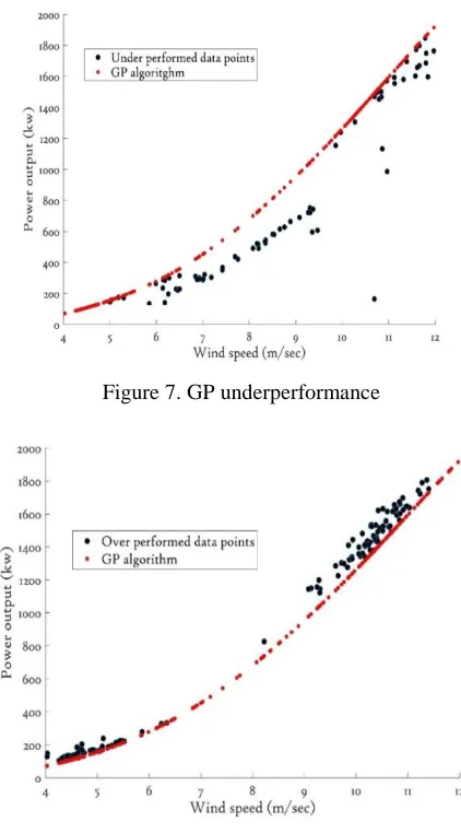
Unhealthy data due to yaw misalignments (described in section 4) used to assess in terms of a probabilistic approach where each new data point compared with the constructed GP reference power curve and if these data points lie outside of the confidence intervals of the GP reference power curve then this indicates anomalous behavior and possible fault; results shown in figure 7. A common cause of turbine underperformance is due to nacelle misalignment, and other reasons such as error due to pitch and controller also contribute to the turbine underperformance, (Alain Bensoussan et al.2014) and (Breno Menezes.2014). The
[image:6.612.326.537.142.523.2]performance assessments, derived from nacelle anemometry which can be misleading; for example, interpreted as over performance (identified by GP model and is shown in figure 8) and these over performance reading is may be due to the control operator sides.
Figure 7. GP underperformance
Figure 8. GP over performance 6.CONCLUSION
data points and computational cost is key to developing effective Gaussian Process algorithms for condition monitoring purposes.
Future work includes considering other nonparametric models for validating GP model effectiveness.
ACKNOWLEDGMENT
This project has received funding from the European Union’s Horizon 2020 research and innovation programme under the Marie Sklodowska-Curie grant agreement No 642108. REFERENCES
Hyers, R. W et al.,2006. Condition Monitoring and Prognosis of Utility Scale Wind Turbines. Energy Materials, vol. 1, no. 3. pp. 187-203.
Zaher, A et al.,2009. Online wind turbine fault detection through automated SCADA data analysis. Wind Energy., 12: 574–593. doi:10.1002/we.319.
Martin, R et al., 2016.Sensitivity analysis of offshore wind farm operation and maintenance cost and availability.
Renewable Energy, 85, pp. 1226-1236.
M. Lydia et al., 2014. A comprehensive review on wind turbine power curve modeling techniques. Renew. Sustain. Energy Rev., 30, pp. 452-460.
S. Shokrzadeh et al., 2014. Wind Turbine Power Curve Modeling Using Advanced Parametric and Nonparametric Methods. IEEE Transactions on Sustainable Energy, vol.5, no.4, pp.1262-269.doi: 10.1109/TSTE.2014.2345059.
Thapar V et al.,2011. Critical analysis of methods for mathematical modelling of wind turbines. Renew Energy,36:3166–77.
http://dx.doi.org/10.1155/2016/8519785.
Leszek Romański et al.,2017. Estimation of operational parameters of the counter-rotating wind turbine with artificial neural networks. Archives of Civil and Mechanical Engineering, Volume 17, Issue 4, Pages 1019-1028.
Lorenzo Dambrosio.,2017. Data-based Fuzzy Logic Control Technique Applied to a Wind System. Energy Procedia, Volume 126, Pages 690-697.
Raik Becker et al.,2017. Completion of wind turbine datasets for wind integration studies applying random forests and k-nearest neighbors. Applied Energy, Volume 208, Pages 252-262.
T. Ouyanga et al.,2017. Modelling wind-turbine power curve: a data partitioning and mining approach Renew. Energy, 01102 (A), pp. 1-8.
Y. Wang & D. Infield.,2013. Supervisory control and data acquisition data-based non-linear state estimation technique for wind turbine gearbox condition monitoring. IET Renewable Power Generation, vol. 7, no. 4, pp. 350-358, doi: 10.1049/iet-rpg.2012.0215.
Y. Si et al.,2017, A data-driven approach for fault detection of offshore wind turbines using random forests. IECON 2017 - 43rd Annual Conference of the IEEE Industrial Electronics Society, Beijing, China, pp. 3149-3154. doi: 10.1109/IECON.2017.8216532.
R. K. Pandit & D. Infield.,2017. Using Gaussian Process theory for wind turbine power curve analysis with emphasis on the confidence intervals. 6th International Conference on Clean Electrical Power (ICCEP), Santa
Margherita Ligure, pp.744-749. doi: 10.1109/ICCEP.2017.8004774.
Neal, R. M.,1994. Bayesian Learning for Neural Networks. PhD thesis, University of Toronto, Canada.
C. E. Rasmussen & C. K. I. Williams., 2006.Gaussian Processes for Machine Learning, the MIT Press, ISBN 026218253X.
Xueru Wang et al.,2014. Wind turbine gearbox forecast using Gaussian Process model. Control and Decision Conference, The 26th Chinese.
Niya Chen et al.,2013. Short-Term Wind Power Forecasting Using Gaussian Processes, Twenty-Third International Joint Conference on Artificial Intelligence.
Kim K et al., 2011. Use of SCADA data for failure detection in wind turbines. Energy Sustainability Conference and Fuel Cell Conference, NREL/CP-5000-51653.
Kusiak A & Zhang Z., 2010. Analysis of wind turbine vibrations based on SCADA data. J Sol Energy Eng. doi:10.1115/1.4001461.
P. Dao et al.,2018. Condition monitoring and fault detection in wind turbines based on cointegration analysis of SCADA data. Renew. Energy, 116 (Part B), pp. 107-122. Zaher AS et al., 2007.A multi-agent fault detection system for wind turbine defect recognition and diagnosis. IEEE Lausanne Power Tech, pp:22–27.
M. Schlechngen & I. F. Santos.,2011. Comparative analysis of neural network and regression based condition monitoring approaches for wind turbine fault detection.
Mech. Syst. Signal Process., vol. 25, no. 5, pp. 1849– 1875.
IEC 61400-12-1., 2006.Wind Turbines—Part 12-1: Power Performance Measurements of Electricity Producing Wind Turbines, British Standard,
Vaishali Sohoni et al.,2016. A Critical Review of Wind Turbine Power Curve Modelling Techniques and Their Applications in Wind Based Energy Systems. Journal of Energy, Article ID 8519785, 18 pages, doi:10.1155/2016/8519785.
Avent lidar technology., 2013. Flexible solutions to optimize turbine performance. Available online at
http://www.aventlidartechnology.com/en/applications/y aw-error-correction_116.html.
J. G. Schepers.,2007. Dynamic Inflow effects at fast pitching steps on a wind turbine placed in the NASA-Ames wind tunnel. ECN Reports.
M. Spencer et al.,2013. Predictive yaw control of a 5MW wind turbine model. AIAA Aerospace Sciences Meeting Including the New Horizons Forum and Aerospace Exposition.
K. A. Kragh & P. Fleming., 2012.Rotor speed dependent yaw control of wind turbines based on empirical data. AIAA Aerospace Sciences Meeting Including the New Horizons Forum and Aerospace Exposition.
Song, D et al., 2017. Wind direction prediction for yaw control of wind turbines. Int. J. Control Autom. Syst. 15: 1720. https://doi.org/10.1007/s12555-017-0289-6. PMO Gebraad et al.,2016. Wind plant power optimization
through yaw control using a parametric model for wake effects—a cfd simulation study. Wind Energy, 19(1):95– 114.
Jinkyoo Park & Kincho H Law., 2015. A Bayesian optimization approach for wind farm power maximization. In SPIE Smart Structures and Materials+ Nondestructive Evaluation and Health Monitoring, pp 943608– 943608. International Society for Optics and Photonics.
Ping Li & Songcan Chen., 2016.Gaussian Process Latent Variable Models. CAAI Transactions on Intelligence Technology. Volume 1, Issue 4, pp 366-376.
J. Hartikainen et al., 2010.Kalman filtering and smoothing solutions to temporal Gaussian Process regression models. IEEE International Workshop on Machine Learning for Signal Processing.
S. Sarkka et al., 2013.Spatiotemporal learning via infinite-dimensional Bayesian filtering and smoothing. IEEE Signal Processing Magazine, vol. 30, no. 4, pp. 51–61. Jie Chen & Nannan Cao., 2013.Parallel Gaussian Process
Regression with Low-Rank Covariance Matrix Approximations. Proceedings of the Twenty-Ninth Conference on Uncertainty in Artificial Intelligence (UAI2013). https://arxiv.org/abs/1408.2060.
Neyman, J., 1937.Outline of a Theory of Statistical Estimation Based on the Classical Theory of Probability.
Philosophical Transactions of the Royal Society A. 236: 333–380. doi:10.1098/rsta.1937.0005.
Alain Bensoussan et al., 2014.Confidence intervals for annual wind power production. ESAIM: Proc., 44,pp 150-158. doi: https://doi.org/10.1051/proc/201444009. Breno Menezes.,2014. Creating Confidence Intervals for
Reservoir Computing’s Wind Power Forecast Use of Maximum Likelihood Method and the Distribution-based Method. COGNITIVE 2014: The Sixth International Conference on Advanced Cognitive Technologies and Applications.
Andrew McHutchon & Carl Edward Rasmussen.,2011. Gaussian Process Training with Input Noise.
http://mlg.eng.cam.ac.uk/mchutchon/papers/NIGP.pdf.
BIOGRAPHIES
Mr Ravi Kumar Pandit is a PhD student under Marie Curie fellowship in the Department of Electronics and Electrical Engineering, University of Strathclyde. Mr Pandit received Bachelor of Engineering in Electrical from Jadavpur University and Master of Technology in Instrumentation Engineering from Indian Institute of Technology, Kharagpur. From April 2014 to Jan 2016, he worked as assistant professor at Jadavpur University. He previously worked as assistant professor in Vellore Institute of Technology (Dec 2011 to April 2014). His areas of Interest Are Instrumentation, Power forecasting, wind turbines O&M and Characteristics Analysis of Wind Speed.