Semi-active structural control of offshore wind turbines considering damage development

(1)

Marine Science

and Engineering

Article

Semi-Active Structural Control of Offshore Wind

Turbines Considering Damage Development

Arash Hemmati and Erkan Oterkus *

Department of Naval Architecture, Ocean & Marine Engineering, University of Strathclyde, Glasgow G4 0LZ, UK; [email protected]

* Correspondence: [email protected]; Tel.: +44-141-548-3876

Received: 29 June 2018; Accepted: 31 August 2018; Published: 5 September 2018

Abstract: High flexibility of new offshore wind turbines (OWT) makes them vulnerable since they are subjected to large environmental loadings, wind turbine excitations and seismic loadings. A control system capable of mitigating undesired vibrations with the potential of modifying its structural properties depending on time-variant loadings and damage development can effectively enhance serviceability and fatigue lifetime of turbine systems. In the present paper, a model for offshore wind turbine systems equipped with a semi-active time-variant tuned mass damper is developed considering nonlinear soil–pile interaction phenomenon and time-variant damage conditions. The adaptive concept of this tuned mass damper assumes slow change in its structural properties. Stochastic wind and wave loadings in conjunction with ground motions are applied to the system. Damages to soil and tower caused by earthquake strokes are considered and the semi-active control device is retuned to the instantaneous frequency of the system using short-time Fourier transformation (STFT). The performance of semi-active time-variant vibration control is compared with its passive counterpart in operational and parked conditions. The dynamic responses for a single seismic record and a set of seismic records are presented. The results show that a semi-active mass damper with a mass ratio of 1% performs significantly better than a passive tuned mass damper with a mass ratio of 4%.

Keywords:offshore wind; structural control; semi-active; tuned mass damper; earthquake

1. Introduction

The wind industry has attracted attention and is growing rapidly due to the environmental concerns over conventional energy resources. The offshore wind industry, in particular, is becoming more attractive because of its advantages over onshore wind. Offshore wind turbines (OWT) are subject to undesirable vibrations caused by environmental loadings, seismic excitations, and rotor frequency excitations, and these excessive vibrations need to be minimized to increase serviceability and lifetime of the system. A number of structural control devices using vibration control mechanisms have been developed to mitigate the aforementioned excessive vibrations. Tuned mass dampers (TMDs) and tuned liquid dampers (TLDs) are two main vibration control devices widely used.

Various vibration control mechanisms originally from civil engineering field have been proposed to control the level of vibrations in the wind industry. Three main vibration control methods such as passive, semi-active, and active exist. The applications and descriptions of these methods utilized in buildings and wind turbine structures were reviewed by Symans and Constantinou [1] and Chen and Georgakis [2]. The passive control system improves damping and stiffness of the main structure without the need of employing external forces [3,4]. The vibrations are not tracked via sensors in this method as curations of this system are constant. This method is widely used due to easy implementation and maintenance. Active vibration control system is a more sophisticated method

(2)

J. Mar. Sci. Eng.2018,6, 102 2 of 22

in which not only mechanical properties are adjusted in the time domain but also external forces are employed. Thus, active control method requires the presence of active forces from external sources, resulting in high cost and complexity of the system. Semi-active vibration control system is the modified version of the passive control system with the capability of adjusting the properties of the system in the time domain with respect to certain properties of vibration forces such as frequency content and amplitudes. Vibration amplitudes and frequencies are tracked down using sensors and signal processing techniques in order to adjust the structural properties. Therefore, semi-active system optimizes vibration control capacity without employing external forces. In other words, semi-active system enjoys the best of both active and passive systems; therefore, it can be a more reliable and economically viable option for offshore wind turbines which are subjected to changes in their natural frequencies.

There is a considerable amount of literature on passive vibration control devices for wind turbines. One of the early studies in this field was done by Enevoldsen and Mørk [5] in which effects of passive tuned mass dampers on a 500 kW wind turbine were studied and a cost-effective design was achieved owing to the implementation of structural control devices. Later on, Murtagh et al. [6] investigated the use of tuned mass dampers (TMD) for mitigating along-wind vibrations of wind turbines. They concluded that the dynamic responses could be reduced providing that the device is tuned to the fundamental frequency. Colwell and Basu [7] examined effects of tuned liquid column dampers (TLCDs) on offshore wind turbine systems to suppress the excessive vibrations and found that TLCD can minimize vibrations up to 55% of peak responses of OWTs compared to the uncontrolled system. Stewart and Lackner [8] examined the impact of passive tuned mass dampers (PTMD) considering wind–wave misalignment on offshore wind turbine loads for monopile foundations. The results demonstrated that TMDs are effective in damage reduction of towers, especially in side–side directions. Stewart and Lackner [9] in another study investigated the effectiveness of TMD systems for four different types of platforms including monopile, barge, spar buoy, and tension-leg and they observed tower fatigue damage reductions of up to 20% for various TMD configurations. In addition, passive multiple tuned mass dampers (MTMD) were proposed to improve the effectiveness of the vibration control system [10]. Dinh and Basu [10] investigated the use of passive MTMDs for structural control of nacelle and tower of spar floating wind turbines and concluded that MTMDs are more effective in displacement reduction. Whilst passive control methods can reduce the dynamic vibrations to some extent provided they are tuned properly, they can be easily off-tuned as soon as the dominating frequency of the system changes, resulting in ineffectiveness of the system and even increased vibrations compared to the uncontrolled system. Highly dynamic nature of offshore wind turbines subjected to a number of dynamic loadings and interacting with nonlinear soil conditions results in fluctuations in fundamental frequency. Abrupt pulsed nature excitations such as earthquake motions can lead to degradation of soil stiffness and, consequently, reduction in natural frequency. Furthermore, the cyclic vibration of surrounding soil can cause natural frequency reduction. In addition, natural frequency increase might occur when there is stiffening phenomena in certain soil types. Therefore, this raises many questions regarding the use of passive control devices in offshore wind turbines for the whole lifetime in which there are variations in dominating frequency and the application of more sophisticated vibration control devices needs to be examined.

(3)

active dynamic vibration absorber. They used a single active electrical dynamic absorber and tested its effectiveness in control of multiple modes both experimentally and analytically.

The semi-active control mechanism is more suitable for the systems with high time-variant parameters such as offshore wind turbines. Semi-active vibration control devices for the application of buildings have been actively studied by a number of researchers [1,19–23] in the last few decades. However, their application in wind energy is a new field. One of the earliest studies on semi-active control mechanism for wind turbines was done by Kirkegaard et al. [24], in which they presented an experimental and numerical investigation of semi-active vibration control of offshore wind turbines equipped with a magnetorheological (MR) fluid damper. The authors claimed that using MR dampers for offshore wind turbines results in considerable reduction of the lateral displacement compared to the uncontrolled system. Later on, Karimi et al. [25] proposed a controllable valve in tuned liquid column dampers for the application of offshore wind turbines. In addition, the use of semi-active tuned mass dampers in control of flapwise vibrations of wind turbines was examined by Arrigan et al. [26]. The authors proposed a frequency-tracking algorithm for retuning the vibration control device and they observed significant vibration reductions owing to the semi-active mechanism. Furthermore, Weber [27] studied application of an adaptive tuned mass damper concept based on semi-active controller using MR dampers. Their results showed that the real-time controlled MR semi-active tuned mass damper is a robust device for reducing structural vibrations. Semi-active control mechanism for tuned liquid column dampers (TLCDs) was also studied by Sonmez et al. [28]. The authors used a control algorithm based on short-time Fourier transformation (STFT) and investigated the effectiveness of the proposed device under random excitations. More recently, Sun [29] explored semi-active tuned mass dampers for the NREL (National Renewable Energy Laboratory) 5 MW baseline wind turbine excited by environmental loadings in conjunction with seismic motions considering post-earthquake damage to soil and tower stiffnesses. The author demonstrated the superiority of semi-active vibration control over the passive one in multihazard conditions. Although Sun’s [29] work is well founded, it is limited to only one earthquake record (1994 Northridge Newhall 90) and further study for a suite of earthquake records with different frequency contents and intensities is required. Another limitation of the aforementioned work is that soil–pile interaction was modeled using a simplified method (closed-form solution) in which the stiffness of embedded pile is considered with a constant rotation and lateral stiffness value in seabed level. More advanced soil–pile interaction model based on time-variant nonlinear stiffness considering soil damage phenomena can enhance the previous works. In addition, the effect of semi-active tuned mass dampers on other structural responses such as base shear and base moment should be investigated.

(4)

J. Mar. Sci. Eng.2018,6, 102 4 of 22

2. Model Description

2.1. Tuned Mass Damper Systems

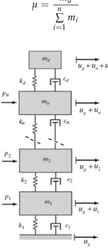
A tuned mass damper (TMD) is a structural control device that consists of a mass, a damper, and a mass attached to a primary structure to control excessive vibration of the primary structure by dissipating energy. The key feature of a TMD is that its frequency is tuned to a particular structural frequency to mitigate the vibrations when that frequency is excited. The theory of multiple degrees of freedom (MDOF) systems using tuned mass dampers are illustrated and presented in the following section.

The governing equations for the MDOF system in Figure1are given as:

m1u1.. +c1u1. +k1u−k2(u2−u1)−c2(u2. −u1. ) =p1−m1u..g

m2u2.. +c2(u2. −u1. ) +k2(u2−u1)−k3(u3−u2)−c3(u3. −u2. ) =p2−m2u..g ..

.

md .. ud+cd

.

ud+kdud=−md( .. un+

..

ug) (1)

wheremi,ci,ki,ui, andpiare mass, damping, stiffness, deflection, and point load for different degrees of freedom of main structure (i = 1, 2, . . . ,n), andmd,cd,kd, andud are mass, damping, stiffness, and deflection for the TMD attached to the primary structure.ugis the absolute ground motion due to seismic loadings. The optimal tuned frequency of the TMD,ωdis defined as:

ωd=γω (2)

in whichωis the natural frequency, andγis the optimal tuning ratio which is determined by the

following formula:

γ= 1

1+µ (3)

whereµis the mass ratio as given by the following formula:

µ= _nmd ∑ i=1

mi

(4)

[image:4.595.243.349.503.745.2]

J. Mar. Sci. Eng. 2018, 6, x 5 of 22

Figure 1. Multi degrees of freedom system equipped with a tuned mass damper (TMD).

The schematic configuration of a TMD inside the nacelle is shown in Figure 2.

Figure 2. Schematic figure of TMD in the nacelle.

2.2. Semi-Active Vibration Control Algorithm

There are three main parameters that define a tuned mass damper: mass, stiffness, and damping. Mass of vibration control device cannot be changed in time domain due to practical reasons and only stiffness and damping of the device are altered in time domain depending on instantaneously structural properties of the system and instant dynamic responses. There have been studies on algorithms for time-variant properties of semi-active tuned mass dampers by [21,23,26,28]. In most of the previous studies, the stiffness of semi-active TMD is tuned according to instantaneously identified frequency using short-time Fourier transform and the damping parameters are modulated based on the TMD deflection in each time step.

2.2.1. Varying Stiffness

Stiffness of the semi-active tuned mass damper can be modified based on the identified dominant frequency using short-time Fourier transformation (STFT) function as suggested in the previous studies such as [27,29,30]. Unlike the standard Fourier transform, short-time Fourier transformation adds a time dimension to the base function parameters. A signal x(τ_{) is multiplied by}

a moving window function as h(τ−t):

(5)

J. Mar. Sci. Eng.2018,6, 102 5 of 22

The schematic configuration of a TMD inside the nacelle is shown in Figure2.

Figure 1. Multi degrees of freedom system equipped with a tuned mass damper (TMD).

[image:5.595.177.423.116.281.2]

The schematic configuration of a TMD inside the nacelle is shown in Figure 2.

Figure 2. Schematic figure of TMD in the nacelle.

2.2. Semi-Active Vibration Control Algorithm

Stiffness of the semi-active tuned mass damper can be modified based on the identified dominant frequency using short-time Fourier transformation (STFT) function as suggested in the previous studies such as [27,29,30]. Unlike the standard Fourier transform, short-time Fourier transformation adds a time dimension to the base function parameters. A signal x(τ_{) is multiplied by} a moving window function as h(τ−t):

Figure 2.Schematic figure of TMD in the nacelle. 2.2. Semi-Active Vibration Control Algorithm

Stiffness of the semi-active tuned mass damper can be modified based on the identified dominant frequency using short-time Fourier transformation (STFT) function as suggested in the previous studies such as [27,29,30]. Unlike the standard Fourier transform, short-time Fourier transformation adds a time dimension to the base function parameters. A signalx(τ) is multiplied by a moving window function ash(τ−t):

ˆ

x(τ) =x(τ)h(τ−t) (5)

in which ˆx(τ)is a weighted signal,τis the moving time andtis the fixed time.

The spectrumS(t,ω)at the fixed time can be defined by applying Fourier transform to ˆx(τ):

S(t,ω) = 1

2π

Z

e−jωt_x_ˆ₌ 1

2π

Z

e−jωt_x₍_τ₎_h₍_τ₋_t₎ ₍₆₎

and the power spectral densityP(t,ω)of timetis calculated as

P(t,ω) =|S(t,ω)|2=S(t,ω).S(t,ω) (7)

Then, the dominant frequency at timetcan be identified using following equations:

ωinst={ω|P(ti,ω) =max{P(ti,ω)} } (8)

ωid = ∑i

k=max{1,i−m+1}ωinst(tk)max{P(tk,ω)} ∑i

k=max{1,i−m+1}max{P(tk,ω)}

(6)

J. Mar. Sci. Eng.2018,6, 102 6 of 22

whereωidis the dominant frequency at timetidetermined through finding the average of instantaneous frequencies overmtime steps (m= 3), andωinstis the instantaneous frequency. In this study, a moving window of 500 time steps (n= 500) with a Hamming window is used. The length of the hamming window is taken 1024,L, resulting in the vector ofPiwith the size ofN×1, whereN= (0.5 *L) + 1. The dominant frequency at each time step is calculated and then stiffness of the tuned mass is retuned using the dominant frequency as

kt_d=kt_d=0(ωid

ωn

)2 (10)

in whichkt_dis the time-variant stiffness of tuned mass damper that can be realized through a variable stiffness device, kt_d=0 is the initial stiffness of tuned mass damper at the time of zero, andωn is the predamage fundamental frequency of the system in which the TMD was tuned to before the development of any damages.

2.2.2. Varying Damping

The damping of tuned mass dampers can be altered according to the dynamic responses in order to increase the effectiveness of the device. In the previous studies by Abe and Igusa [31], the authors investigated the time-variant damping for tuned mass dampers and concluded that TMD can improve its performance if the damping of TMD is time-dependent in such a way that its damping value changes to zero for the duration in which the relative displacement of TMD is increasing. This results in an increase in the efficiency of the system for controlling excessive vibrations. This time-dependent damping algorithm has been used in other works [23,29,32]. In this method, the relative displacement of TMD is tracked in each time step and if it is larger than that of the previous time step, the damping of TMD is set to zero,cdt = 0; otherwise the damping value is set to 2copt,cdt = 2copt. coptis the optimal value of TMD’s damping which can be determined from an estimation method suggested by Sadek et al. [33].

2.3. NREL 5 MW Wind Turbine

The 5 MW NREL wind turbine is considered as it is widely used as the turbine for benchmark studies [34]. This turbine is supported by the baseline monopile foundation developed in the second phase of Offshore Code Comparison (OC3) project conducted by NREL [35]. The geometric configuration of the turbine is shown in Figure 3. The tower and monopile are modeled by three-dimensional Timoshenko beam theory.

(7)

J. Mar. Sci. Eng.2018,6, 102 7 of 22 2.3. NREL 5 MW Wind Turbine

[image:7.595.196.397.85.397.2]

The 5 MW NREL wind turbine is considered as it is widely used as the turbine for benchmark studies [34]. This turbine is supported by the baseline monopile foundation developed in the second phase of Offshore Code Comparison (OC3) project conducted by NREL [35]. The geometric configuration of the turbine is shown in Figure 3. The tower and monopile are modeled by three-dimensional Timoshenko beam theory.

Figure 3. Schematic configuration of the offshore wind turbine.

[image:7.595.86.506.453.586.2]

The particulars of the offshore wind turbine are listed in Table 1. Table 2 provides the material properties of the steel used in the tower and monopile of the offshore wind turbine. To consider additional weight of welds, bolts, and paint, the density of the steel in the tower is assumed 8% higher than that of the regular steel based on the value given in [34].

Table 1. Properties of NREL 5 MW baseline turbine.

Turbine Rated Power, Rotor Orientation 5 MW, Upwind, 3 Blades

Control System Variable Speed, Collective Pitch Blade Rotor Diameter, Hub Height 126 m, 90 m

Cut-In, Rated, Cut-Out Wind Speed 3 m/s, 11.4 m/s, 25 m/s Cut-In, Rated Rotor Speed 6.9 rpm, 12.1 rpm

Hub mass, Blade mass 56,780 kg, 17,740 kg Nacelle Nacelle Dimensions 18 m × 6 m × 6 m

Nacelle Mass 240,000 kg

Tower Base diameter, base thickness 6.0 m, 27 mm Top diameter, top thickness 3.87 m, 19 mm

Tower mass 347,460 kg

Figure 3.Schematic configuration of the offshore wind turbine. Table 1.Properties of NREL 5 MW baseline turbine.

Turbine Rated Power, Rotor Orientation 5 MW, Upwind, 3 Blades

Control System Variable Speed, Collective Pitch

Blade Rotor Diameter, Hub Height 126 m, 90 m

Cut-In, Rated, Cut-Out Wind Speed 3 m/s, 11.4 m/s, 25 m/s Cut-In, Rated Rotor Speed 6.9 rpm, 12.1 rpm

Hub mass, Blade mass 56,780 kg, 17,740 kg

Nacelle Nacelle Dimensions 18 m×6 m×6 m

Nacelle Mass 240,000 kg

Tower Base diameter, base thickness 6.0 m, 27 mm

Top diameter, top thickness 3.87 m, 19 mm

Tower mass 347,460 kg

Table 2.Material properties.

Component Density (kg/m3) Young’s Modulus (GPa) Poisson’s Ratio

Tower 8500 210 0.3

Monopile 7850 210 0.3

2.4. Soil–Pile Interaction

The nonlinear lateral soil resistance–deflection relationship for sand layers can be defined by a hyperbolic tangent function [36]:

P=Aputanh

kH Apuy

(8)

J. Mar. Sci. Eng.2018,6, 102 8 of 22

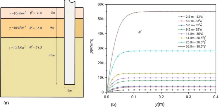
wherePis the soil reaction at a given depth, Ais a calibration factor which equals to 0.9 for cyclic loading, y is the lateral deflection of soil layers, andkis the initial stiffness coefficient which is determined from a function of the angle of internal friction,φ0[36].His depth andpuis the ultimate lateral bearing capacity determined by the following equation:

pu=min (

pus= (C1H+C2D)γH

pud =C3DγH (12)

wherepusis shallow ultimate resistance,pudis deep ultimate resistance,Dis the pile diameter,

γis the effective soil weight, andC1,C2, andC3are coefficients determined from API standard [36].

Soil layer properties are shown in Figure4a. The nonlinear resistance–deflection curves constructed based on the aforementioned method for different soil depths and layers (top, middle, and bottom of each layer) are illustrated in Figure4b.

J. Mar. Sci. Eng. 2018, 6, x 8 of 22

Table 2. Material properties.

Component Density (kg/m3_{) Young’s Modulus (GPa) Poisson’s Ratio}

Tower 8500 210 0.3

Monopile 7850 210 0.3

2.4. Soil–Pile Interaction

The nonlinear lateral soil resistance–deflection relationship for sand layers can be defined by a hyperbolic tangent function [36]:

tanh u

u kH

P Ap y

Ap =



_



_





(11)

where

P

is the soil reaction at a given depth,

A

is a calibration factor which equals to 0.9 for cyclic loading, _{y is the lateral deflection of soil layers, and}_k is the initial stiffness coefficient which is

determined from a function of the angle of internal friction,

φ

′

[36]. H is depth and

p

_u is the ultimate lateral bearing capacity determined by the following equation:

   = + = = H D C p H ) D C H C ( p min p 3 ud 2 1 us u

_γ

γ

(12)

where

p

_us is shallow ultimate resistance,

p

_ud is deep ultimate resistance, D is the pile diameter, _γ

is the effective soil weight, and C₁, C₂, and C₃ are coefficients determined from API standard [36].

[image:8.595.108.490.277.466.2]

Soil layer properties are shown in Figure 4a. The nonlinear resistance–deflection curves constructed based on the aforementioned method for different soil depths and layers (top, middle, and bottom of each layer) are illustrated in Figure 4b.

Figure 4. (a)Soil layer properties, (b) nonlinear lateral resistance–deflection curves.

3. Loading

Stochastically generated wind and wave loadings in conjunction with seismic motions are applied to the structure. Each of these loadings is introduced as follows.

3.1. Wind

Wind loading is the main external force as it generates large overturning moments due to its long moment arm, especially for offshore wind turbines with high hub heights. The wind speed acting on the system can be represented by a constant mean wind load

v

and a turbulent wind

Figure 4.(a) Soil layer properties, (b) nonlinear lateral resistance–deflection curves. 3. Loading

Stochastically generated wind and wave loadings in conjunction with seismic motions are applied to the structure. Each of these loadings is introduced as follows.

3.1. Wind

Wind loading is the main external force as it generates large overturning moments due to its long moment arm, especially for offshore wind turbines with high hub heights. The wind speed acting on the system can be represented by a constant mean wind loadvand a turbulent wind component ˆv(t), v(t) =v+vˆ(t). In this work, the mean wind velocityv(z)as a function of height is determined by means of a logarithmic law as [37]:

v(z) =Vre f

ln(z/z0) ln(Hre f/z0)

(13)

whereVre f is the mean wind velocity at the reference heightHre f =90 m,zis the vertical coordinate, andz0is a surface roughness length parameter.

(9)

mean wind speed. Kaimal spectrumSv(f)[38] is adopted in this study to calculate the turbulent wind velocity as follows:

Sv(f) = 4I 2_L

k (1+6f Lk/v)5/3

(14)

whereIis the wind turbulence intensity,f is the frequency (Hz), andLkis an integral length scale parameter. In this study, the stochastic wind profile is generated using Turbsim code [39] over a rectangular grid with 961 points (31×31) based on Equations (13) and (14). Then, the aerodynamic loadings on the blades are computed in FAST (Version 8.15, NREL, Golden, CO, USA) [40] code using the aforementioned wind profile based on blade element momentum (BEM) theory. Finally, the generated wind loading time history is used in the developed code to consider aerodynamic loadings.

3.2. Sea Wave Load

Wave loading acting on cylindrical structural members of fixed platforms can be obtained using Morison’s equation [37] as the sum of inertia and drag forces. The transverse sea wave force acting on a strip of a lengthdzis given by the sum of inertia and drag force terms as the following equation [41]:

dF= ρw

2 CdDυ|υ|dz+

πD2

2 Cmρw .

υdz (15)

whereCdandCmare the drag and inertia coefficients, respectively (Cd=1.2 andCm=2 in the current study), Dis the diameter of the member, υ. andυare horizontal acceleration and velocity of fluid

particles induced by wave excitations, andρwis water density (1025 kg/m3).

The spectrum developed through the Joint North Sea Wave Observation Project (JONSWAP) is used to generate wave time histories [42] as follows:

Sηη(f) = αg2

f5 exp

−5

4( fm

f ) 4

γ

exp[−(f−fm)2

2σ2fm2 ] ₍₁₆₎

in whichSηη(f)is JONSWAP spectrum,ηis the function of water surface elevation,γis the peak

enhancement factor (3.3 for the north sea),gis the acceleration of gravity, and f is the wave frequency (Hz). The constants in this equation can be defined as

α=0.076

U102/Fg0.22 (17)

fm=11(v10F/g2)

−1/3

/π (18)

and

σ=

( 0.07, 0.09,

f ≤ fm

f > fm (19)

whereU10is the mean wind velocity at 10 m from the sea surface, andFis the fetch length in which the wind blows without any change of direction.

Then, total wave force acting on the structural members can be calculated as

Ff(t) = Z d

0 dFφf

(z)dz (20)

(10)

J. Mar. Sci. Eng.2018,6, 102 10 of 22

3.3. Seismic Excitation

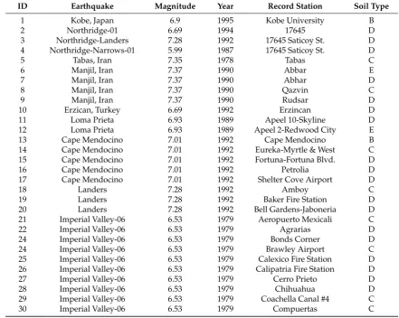
[image:10.595.74.516.225.577.2]

To simulate seismic excitations on the offshore wind turbines, time series of acceleration of strong ground motions during past earthquake events are used. Two horizontal directions are selected to represent the behavior of earthquake events. In this study, sloshing of water surrounding the structure is ignored as it is believed to have insignificant effects. The seismic records are selected from the Pacific Earthquake Engineering Research centre (PEER) Database [43] and listed in Table3. The magnitudes of the seismic ground motions selected in this study vary between 5.5 and 7.5.

Table 3.Seismic records.

ID Earthquake Magnitude Year Record Station Soil Type

1 Kobe, Japan 6.9 1995 Kobe University B

2 Northridge-01 6.69 1994 17645 D

3 Northridge-Landers 7.28 1992 17645 Saticoy St. D

4 Northridge-Narrows-01 5.99 1987 17645 Saticoy St. D

5 Tabas, Iran 7.35 1978 Tabas C

6 Manjil, Iran 7.37 1990 Abbar E

7 Manjil, Iran 7.37 1990 Abhar D

8 Manjil, Iran 7.37 1990 Qazvin C

9 Manjil, Iran 7.37 1990 Rudsar D

10 Erzican, Turkey 6.69 1992 Erzincan D

11 Loma Prieta 6.93 1989 Apeel 10-Skyline D

12 Loma Prieta 6.93 1989 Apeel 2-Redwood City E

13 Cape Mendocino 7.01 1992 Cape Mendocino B

14 Cape Mendocino 7.01 1992 Eureka-Myrtle & West C

15 Cape Mendocino 7.01 1992 Fortuna-Fortuna Blvd. D

16 Cape Mendocino 7.01 1992 Petrolia D

17 Cape Mendocino 7.01 1992 Shelter Cove Airport D

18 Landers 7.28 1992 Amboy C

19 Landers 7.28 1992 Baker Fire Station D

20 Landers 7.28 1992 Bell Gardens-Jaboneria D

21 Imperial Valley-06 6.53 1979 Aeropuerto Mexicali C

22 Imperial Valley-06 6.53 1979 Agrarias D

24 Imperial Valley-06 6.53 1979 Bonds Corner D

24 Imperial Valley-06 6.53 1979 Brawley Airport C

25 Imperial Valley-06 6.53 1979 Calexico Fire Station D

26 Imperial Valley-06 6.53 1979 Calipatria Fire Station D

27 Imperial Valley-06 6.53 1979 Cerro Prieto D

28 Imperial Valley-06 6.53 1979 Chihuahua D

29 Imperial Valley-06 6.53 1979 Coachella Canal #4 C

30 Imperial Valley-06 6.53 1979 Compuertas C

4. Numerical Results and Discussions

4.1. Model Verification

(11)

[image:11.595.113.484.111.176.2]

J. Mar. Sci. Eng.2018,6, 102 11 of 22

Table 4.Natural frequency analysis results (Hz).

Mode Code ANSYS Dong Hywan Kim et al. [45]

1nd Fore–aft 0.235 0.234 0.234

1nd Side-to-side 0.235 0.234 0.233

2nd Fore–aft 1.426 1.426 1.406

2nd Side-to-side 1.426 1.426 1.515

Then, a dynamic analysis for the offshore wind turbine subjected to a single earthquake motion (Northridge) is carried out and the results are compared with the results obtained from the dynamic analysis performed in ANSYS. Figure5a shows the nonscaled time history of acceleration of Northridge earthquake starting from the instant of 50 s. Figure 5b illustrates the time history of nacelle displacement simulated with the code written in MATLAB and the corresponding results obtained from ANSYS and good matches are observed.

4. Numerical Results and Discussions

4.1. Model Verification

In this section, the results of the natural frequency and dynamic analyses using the developed model in MATLAB (R2017a, MathWorks, Natick, MA, USA) are verified. To carry out natural frequency analysis, the stiffness of nonlinear soil–pile interaction is linearized by taking initial stiffness of the p–y curves [44]. The resulting first and second natural frequencies are listed in Table 4 and compared with the results of the model created by commercial finite element software ANSYS (16, Canonsburg, PA, USA) and the results from the literature [45]. There is good agreement between the results of natural frequency analyses.

Table 4. Natural frequency analysis results (Hz).

Mode Code ANSYS Dong Hywan Kim et al. [45] 1nd Fore–aft 0.235 0.234 0.234

1nd Side-to-side 0.235 0.234 0.233 2nd Fore–aft 1.426 1.426 1.406 2nd Side-to-side 1.426 1.426 1.515

Then, a dynamic analysis for the offshore wind turbine subjected to a single earthquake motion (Northridge) is carried out and the results are compared with the results obtained from the dynamic analysis performed in ANSYS. Figure 5a shows the nonscaled time history of acceleration of Northridge earthquake starting from the instant of 50 s. Figure 5b illustrates the time history of nacelle displacement simulated with the code written in MATLAB and the corresponding results obtained from ANSYS and good matches are observed.

Figure 5. (a) Time history of acceleration of seismic excitation (Northridge), (b) time history of the nacelle displacement simulated with ANSYS and the developed code under seismic excitation (Northridge).

4.2. Damage Development

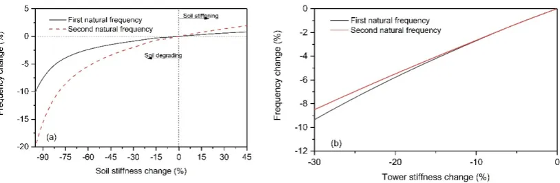
[image:11.595.101.493.288.413.2]

Dynamic performance of passive tuned mass dampers is threatened by changes in the natural frequency of the system. This change in the natural frequency can occur either gradually over the lifetime of the system due to soil degradation under long-term cyclic loading or rapidly over a short period of time due to seismic excitation. Figure 6a shows the effect of soil stiffness changes (damage or stiffening in soil) on the first and second natural frequency of the system. The Figure shows that a 50% reduction in soil stiffness leads to 2.2%, and 4.8% reduction in the first and second natural frequencies of the system, respectively. The Figure indicates that the second natural frequency changes more and degradation of soil stiffness has a larger effect on the frequency change rather than stiffening of soil. Similarly, the frequency change of the system due to tower damage is shown in Figure 6b. The Figure suggests that tower damage reduces the natural frequency to a greater extent.

Figure 5. (a) Time history of acceleration of seismic excitation (Northridge), (b) time history of the nacelle displacement simulated with ANSYS and the developed code under seismic excitation (Northridge).

4.2. Damage Development

(12)

J. Mar. Sci. Eng.2018,6, 102 12 of 22

J. Mar. Sci. Eng. 2018, 6, x 12 of 22

[image:12.595.96.503.87.220.2]

For example, 20% stiffness reduction of tower leads to 5.9% decrease in the first natural frequency of the system.

Figure 6. Frequency change due to (a) soil degrading/stiffening, (b) tower stiffness reduction.

[image:12.595.101.497.407.534.2]

The degradation stiffness model of monopile foundations under long-term cyclic loading was studied by Martin Achmus et al. [46]. Sun also considered soil and tower stiffness damage development for seismic loading using simplified linear stiffness reduction scenarios [29]. In this study, a rapid degradation stiffness model is assumed as the focus of the study is on the short-term damage development due to seismic excitation. Therefore, the damage development model similar to Sun [29] is assumed with the values in which a 5% reduction in natural frequency occurs. To model damage development, it is assumed that damage begins developing at the start of earthquake and soil stiffness and tower stiffness reduces linearly in 20 s as depicted in Figure 7. Tower stiffness and tower stiffness are assumed to reduce 30% and 15%, respectively. The reduction in the stiffness of the tower is assumed in the whole tower.

Figure 7. Damage development: (a) soil stiffness, (b) tower stiffness.

4.3. Response to a Single Seismic Record

To give a preliminary insight into the dynamic responses of offshore wind turbines equipped with semi-active and passive tuned mass dampers considering frequency change as a result of damage development, the responses to a single seismic record for different loading conditions are discussed in this section. Four loading conditions are adopted according to IEC (International Electrotechnical Commission) standards [47] and their properties are tabulated in Table 5. In the first loading condition scenario (LC1), the turbine is operating under steady wind loading at the rated wind speed. In the second loading condition (LC2), the parked turbine is subjected to a steady wind speed of 40 m/s. For both of these loading conditions, there is no wave loading which represents calm sea conditions. Loading conditions LC3 and LC4 are the same as LC1 and LC2 but with stochastic wind and wave loadings. For all these loading conditions, the seismic event in conjunction with damage development occurs at the instant of 50 s.

Figure 6.Frequency change due to (a) soil degrading/stiffening, (b) tower stiffness reduction.

The degradation stiffness model of monopile foundations under long-term cyclic loading was studied by Martin Achmus et al. [46]. Sun also considered soil and tower stiffness damage development for seismic loading using simplified linear stiffness reduction scenarios [29]. In this study, a rapid degradation stiffness model is assumed as the focus of the study is on the short-term damage development due to seismic excitation. Therefore, the damage development model similar to Sun [29] is assumed with the values in which a 5% reduction in natural frequency occurs. To model damage development, it is assumed that damage begins developing at the start of earthquake and soil stiffness and tower stiffness reduces linearly in 20 s as depicted in Figure7. Tower stiffness and tower stiffness are assumed to reduce 30% and 15%, respectively. The reduction in the stiffness of the tower is assumed in the whole tower.

J. Mar. Sci. Eng. 2018, 6, x 12 of 22

For example, 20% stiffness reduction of tower leads to 5.9% decrease in the first natural frequency of the system.

Figure 6. Frequency change due to (a) soil degrading/stiffening, (b) tower stiffness reduction.

The degradation stiffness model of monopile foundations under long-term cyclic loading was studied by Martin Achmus et al. [46]. Sun also considered soil and tower stiffness damage development for seismic loading using simplified linear stiffness reduction scenarios [29]. In this study, a rapid degradation stiffness model is assumed as the focus of the study is on the short-term damage development due to seismic excitation. Therefore, the damage development model similar to Sun [29] is assumed with the values in which a 5% reduction in natural frequency occurs. To model damage development, it is assumed that damage begins developing at the start of earthquake and soil stiffness and tower stiffness reduces linearly in 20 s as depicted in Figure 7. Tower stiffness and tower stiffness are assumed to reduce 30% and 15%, respectively. The reduction in the stiffness of the tower is assumed in the whole tower.

Figure 7. Damage development: (a) soil stiffness, (b) tower stiffness.

4.3. Response to a Single Seismic Record

To give a preliminary insight into the dynamic responses of offshore wind turbines equipped with semi-active and passive tuned mass dampers considering frequency change as a result of damage development, the responses to a single seismic record for different loading conditions are discussed in this section. Four loading conditions are adopted according to IEC (International Electrotechnical Commission) standards [47] and their properties are tabulated in Table 5. In the first loading condition scenario (LC1), the turbine is operating under steady wind loading at the rated wind speed. In the second loading condition (LC2), the parked turbine is subjected to a steady wind speed of 40 m/s. For both of these loading conditions, there is no wave loading which represents calm sea conditions. Loading conditions LC3 and LC4 are the same as LC1 and LC2 but with stochastic wind and wave loadings. For all these loading conditions, the seismic event in conjunction with damage development occurs at the instant of 50 s.

Figure 7.Damage development: (a) soil stiffness, (b) tower stiffness. 4.3. Response to a Single Seismic Record

(13)

[image:13.595.79.514.111.190.2]

Table 5.Loading condition (LC) information.

Wind Wave Seismic

Loadcases Wind Speed at the Hub Height (m/s)

Turbulence Intensity (%)

Wave Period (s)

Significant Wave Height (m)

Starting

Instant Damping

LC1 11.4 (Operational) 0 - - 50 s 1%

LC2 40.0 (Parked) 0 - - 50 s 5%

LC3 11.4 (Operational) 14.5 9.5 5.0 50 s 1%

LC4 40.0 (Parked) 11.7 11.5 7.0 50 s 5%

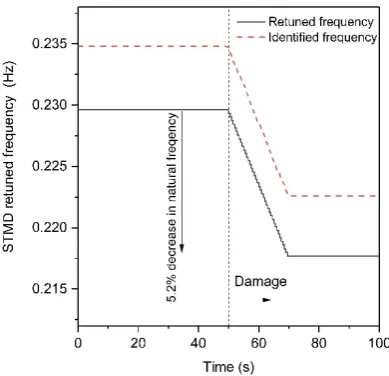
The identified dominant frequency according to short-time Fourier transport function is calculated in each time step and the stiffness of semi-active tuned mass damper is retuned according to Equation (10). The identified dominant frequency and retuned frequencies are depicted in Figure8. The reason that they are not equal is that the optimal tuning ratio,γ, is multiplied by the identified frequency in order to obtain the optimal retuned frequency of TMD. The figure shows that there is 5.2% reduction in the natural frequency of the system and consequently retuned frequency of tuned mass damper. This retuned frequency can be realized with 10% decrease in the stiffness of tuned mass damper.

Table 5. Loading condition (LC) information.

Wind Wave Seismic

Loadcases Wind Speed at the Hub Height (m/s)

Turbulence Intensity (%)

Wave Period (s)

Significant Wave Height

(m)

Starting

Instant Damping

LC1 11.4 (Operational) 0 - - 50 s 1%

LC2 40.0 (Parked) 0 - - 50 s 5%

LC3 11.4 (Operational) 14.5 9.5 5.0 50 s 1%

LC4 40.0 (Parked) 11.7 11.5 7.0 50 s 5%

[image:13.595.200.395.324.512.2]

The identified dominant frequency according to short-time Fourier transport function is calculated in each time step and the stiffness of semi-active tuned mass damper is retuned according to Equation (10). The identified dominant frequency and retuned frequencies are depicted in Figure 8. The reason that they are not equal is that the optimal tuning ratio, γ, is multiplied by the identified frequency in order to obtain the optimal retuned frequency of TMD. The figure shows that there is 5.2% reduction in the natural frequency of the system and consequently retuned frequency of tuned mass damper. This retuned frequency can be realized with 10% decrease in the stiffness of tuned mass damper.

Figure 8. Retuned frequency of semi-active tuned mass damper (STMD).

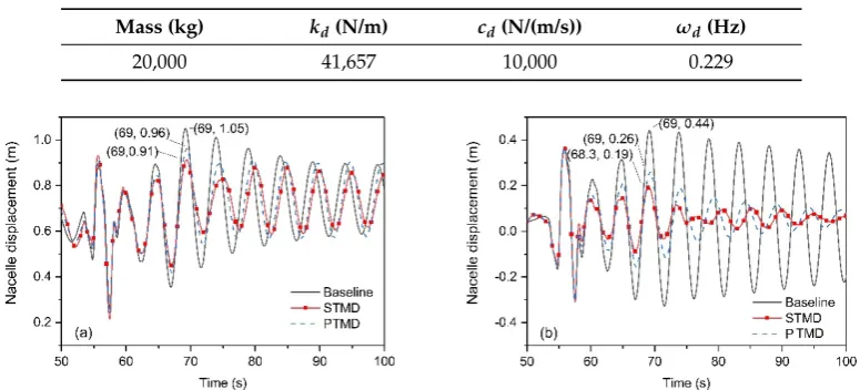
The dynamic responses of the offshore wind turbine subjected to a single seismic record (Kobe) are discussed here. In the following section, baseline denotes uncontrolled system. For the controlled systems, PTMD and STMD denote passive TMD and semi-active TMD, respectively. The parameters of the tuned mass dampers used in this section are tabulated in Table 6. Figure 9 compares the nacelle displacement responses of the turbine under steady wind loadings. At first glance, it is clear that for LC1 and LC2, STMD is superior to PTMD. In Figure 9a, the peak of nacelle displacement decreased from 0.96 m to 0.91 m for operational loading LC1 and the dynamic response of PTMD is nearly as much as the baseline system especially after the end of earthquake and damage development. This shows that the PTMD becomes off-tuned and unable to control the vibration. However, STMD can retune to the new frequency and mitigate the dynamic responses. The displacement reductions are more pronounced for the parked condition (LC2) in which the peak of nacelle displacement for STMD is 0.19 m compared to 0.26 m of the passive tuned mass damper, nearly 16% more reductions compared to the baseline system.

Figure 8.Retuned frequency of semi-active tuned mass damper (STMD).

(14)

[image:14.595.103.491.107.283.2]

J. Mar. Sci. Eng.2018,6, 102 14 of 22

Table 6.TMD parameters.

Mass (kg) kd(N/m) cd(N/(m/s)) ωd(Hz)

20,000 41,657 10,000 0.229

J. Mar. Sci. Eng. 2018, 6, x 14 of 22

Table 6. TMD parameters.

Mass (kg) kd(N/m) cd (N/(m/s)) ωd (Hz)

20,000 41,657 10,000 0.229

Figure 9. Time history of nacelle displacement under steady wind loading and seismic excitation considering damage development. (a) LC1, (b) LC2. PTMD: passive tuned mass damper.

To scrutinize the energy spectrum of dynamic responses, the power spectral density (PSD) of the nacelle displacements for LC1 and LC2 is obtained and presented in Figure 10. Fast Fourier transformation based on Hamming window is used to capture a smooth PSD curve. Figure 10a indicates that there are two distinct peaks corresponding to the energy of wind loading and turbine frequency (1P) whose frequencies are around zero and 0.2 Hz, respectively. It is clear that the PSD for energy from wind loading (frequencies close to zero) shows negligible changes for PTMD and STMD as these devices are tuned to the first natural frequency of the system. However, a 37% reduction in the peak of the power spectrum for the STMD system can be observed for the turbine frequency (1P). Similarly, power spectral density of the nacelle displacement for LC2 (parked condition) is shown in Figure 10b. Compared to the operational condition (Figure 10a), energy spectrum corresponding to frequency of wind loading (close to zero) has much lower peak due to the fact that in parked condition the turbine absorbs a small portion of wind loading as a result of pitching mechanism in the blades and the energy is concentrated around the frequency range of first natural frequency of structure. This is expected because in the parked condition the vibration of structural modes dominates compared to the operational condition where the vibration due to external excitations dominates. The Figure also indicates that the peak of spectrum for the STMD system is reduced as much as 92% compared to the baseline system (uncontrolled system). However, this percentage reduction is lower for the PTMD with 76% reduction. These reductions for both PTMD and STMD are higher in the parked condition (Figure 10b) compared to the operational condition (Figure 10a) because in the parked conditions the aerodynamic damping is negligible and these structural control devices compensate for low total damping value of the system.

Figure 10. Power spectral density (PSD) of nacelle displacement under steady wind loading and seismic excitation considering damage development. (a) LC1, (b) LC2.

To scrutinize the energy spectrum of dynamic responses, the power spectral density (PSD) of the nacelle displacements for LC1 and LC2 is obtained and presented in Figure10. Fast Fourier transformation based on Hamming window is used to capture a smooth PSD curve. Figure10a indicates that there are two distinct peaks corresponding to the energy of wind loading and turbine frequency (1P) whose frequencies are around zero and 0.2 Hz, respectively. It is clear that the PSD for energy from wind loading (frequencies close to zero) shows negligible changes for PTMD and STMD as these devices are tuned to the first natural frequency of the system. However, a 37% reduction in the peak of the power spectrum for the STMD system can be observed for the turbine frequency (1P). Similarly, power spectral density of the nacelle displacement for LC2 (parked condition) is shown in Figure10b. Compared to the operational condition (Figure10a), energy spectrum corresponding to frequency of wind loading (close to zero) has much lower peak due to the fact that in parked condition the turbine absorbs a small portion of wind loading as a result of pitching mechanism in the blades and the energy is concentrated around the frequency range of first natural frequency of structure. This is expected because in the parked condition the vibration of structural modes dominates compared to the operational condition where the vibration due to external excitations dominates. The Figure also indicates that the peak of spectrum for the STMD system is reduced as much as 92% compared to the baseline system (uncontrolled system). However, this percentage reduction is lower for the PTMD with 76% reduction. These reductions for both PTMD and STMD are higher in the parked condition (Figure10b) compared to the operational condition (Figure10a) because in the parked conditions the aerodynamic damping is negligible and these structural control devices compensate for low total damping value of the system.

(15)

J. Mar. Sci. Eng.2018,6, 102 15 of 22

Table 6. TMD parameters.

Mass (kg) kd(N/m) cd (N/(m/s)) ωd (Hz)

20,000 41,657 10,000 0.229

To scrutinize the energy spectrum of dynamic responses, the power spectral density (PSD) of the nacelle displacements for LC1 and LC2 is obtained and presented in Figure 10. Fast Fourier transformation based on Hamming window is used to capture a smooth PSD curve. Figure 10a indicates that there are two distinct peaks corresponding to the energy of wind loading and turbine frequency (1P) whose frequencies are around zero and 0.2 Hz, respectively. It is clear that the PSD for energy from wind loading (frequencies close to zero) shows negligible changes for PTMD and STMD as these devices are tuned to the first natural frequency of the system. However, a 37% reduction in the peak of the power spectrum for the STMD system can be observed for the turbine frequency (1P). Similarly, power spectral density of the nacelle displacement for LC2 (parked condition) is shown in Figure 10b. Compared to the operational condition (Figure 10a), energy spectrum corresponding to frequency of wind loading (close to zero) has much lower peak due to the fact that in parked condition the turbine absorbs a small portion of wind loading as a result of pitching mechanism in the blades and the energy is concentrated around the frequency range of first natural frequency of structure. This is expected because in the parked condition the vibration of structural modes dominates compared to the operational condition where the vibration due to external excitations dominates. The Figure also indicates that the peak of spectrum for the STMD system is reduced as much as 92% compared to the baseline system (uncontrolled system). However, this percentage reduction is lower for the PTMD with 76% reduction. These reductions for both PTMD and STMD are higher in the parked condition (Figure 10b) compared to the operational condition (Figure 10a) because in the parked conditions the aerodynamic damping is negligible and these structural control devices compensate for low total damping value of the system.

[image:15.595.100.500.87.219.2]

Figure 10. Power spectral density (PSD) of nacelle displacement under steady wind loading and seismic excitation considering damage development. (a) LC1, (b) LC2.

J. Mar. Sci. Eng. 2018, 6, x 15 of 22

Figure 11 compares the nacelle displacement responses of the turbine under stochastic wave– wave loadings in conjunction with seismic ground motion and damage development (LC3 and LC4). Again it can be seen that the STMD system shows a better performance in mitigating vibrations and reducing peak displacements. For example, the peak value of displacement is decreased from 1.5 m of the baseline system to 1.27 m of the STMD system for the operational condition (LC3), with 15% reduction. This reduction percentage for the PTMD system is lower, as much as only 6%. Therefore, the STMD’s effectiveness in reducing the peak values is more than twice that of the PTMD. For the parked condition (LC4), higher vibration reductions are observed. For example, the peak nacelle displacement reduced from 1.91 m to 1.01 m as a result of the implementation of the semi-active tuned mass damper. This means that the semi-active achieves 47% reduction in the peak nacelle displacement.

Figure 11. Time history of nacelle displacement under stochastic wind–wave loadings and seismic excitation considering damage development. (a) LC3, (b) LC4.

[image:15.595.101.498.270.393.2]

Looking into power spectral density of the nacelle displacement for LC3 and LC4 in Figure 12, some energy is concentrated around the frequency of 0.1 Hz that corresponds to the energy of wave loadings. Similar to Figure 10, more PSD reduction is observed for parked condition (LC4). However, the difference between the reduction in PSD for PTMD and STMD is less than 10%.

Figure 12. PSD of nacelle displacement under stochastic wind–wave loadings and seismic excitations considering damage development. (a) LC3, (b) LC4.

Figures 13 and 14 show a representative 50 s window time history of the base shear force for steady (LC1 and LC2) and stochastic loadings (LC3 and LC4), respectively. For steady wind loadings (LC1 and LC2), larger base shear is obtained during ground motion and both passive and semi-active TMDs have slight effects on the dynamic responses during the ground motion and damage development. However, the displacements after the damage development are reduced owing to the vibration control devices. For both load cases, STMD is superior to the PTMD. On the other hand, for stochastic loading (Figure 14), changes in the base shear due to tuned mass dampers are insignificant.

Looking into power spectral density of the nacelle displacement for LC3 and LC4 in Figure12, some energy is concentrated around the frequency of 0.1 Hz that corresponds to the energy of wave loadings. Similar to Figure10, more PSD reduction is observed for parked condition (LC4). However, the difference between the reduction in PSD for PTMD and STMD is less than 10%.

J. Mar. Sci. Eng. 2018, 6, x 15 of 22

Figure 11 compares the nacelle displacement responses of the turbine under stochastic wave– wave loadings in conjunction with seismic ground motion and damage development (LC3 and LC4). Again it can be seen that the STMD system shows a better performance in mitigating vibrations and reducing peak displacements. For example, the peak value of displacement is decreased from 1.5 m of the baseline system to 1.27 m of the STMD system for the operational condition (LC3), with 15% reduction. This reduction percentage for the PTMD system is lower, as much as only 6%. Therefore, the STMD’s effectiveness in reducing the peak values is more than twice that of the PTMD. For the parked condition (LC4), higher vibration reductions are observed. For example, the peak nacelle displacement reduced from 1.91 m to 1.01 m as a result of the implementation of the semi-active tuned mass damper. This means that the semi-active achieves 47% reduction in the peak nacelle displacement.

[image:15.595.107.492.510.637.2]

Looking into power spectral density of the nacelle displacement for LC3 and LC4 in Figure 12, some energy is concentrated around the frequency of 0.1 Hz that corresponds to the energy of wave loadings. Similar to Figure 10, more PSD reduction is observed for parked condition (LC4). However, the difference between the reduction in PSD for PTMD and STMD is less than 10%.

Figure 12. PSD of nacelle displacement under stochastic wind–wave loadings and seismic excitations considering damage development. (a) LC3, (b) LC4.

Figures 13 and 14 show a representative 50 s window time history of the base shear force for steady (LC1 and LC2) and stochastic loadings (LC3 and LC4), respectively. For steady wind loadings (LC1 and LC2), larger base shear is obtained during ground motion and both passive and semi-active TMDs have slight effects on the dynamic responses during the ground motion and damage development. However, the displacements after the damage development are reduced owing to the vibration control devices. For both load cases, STMD is superior to the PTMD. On the other hand, for stochastic loading (Figure 14), changes in the base shear due to tuned mass dampers are insignificant.

Figure 12.PSD of nacelle displacement under stochastic wind–wave loadings and seismic excitations considering damage development. (a) LC3, (b) LC4.

(16)

J. Mar. Sci. Eng.2018,6, 102 16 of 22

devices. For both load cases, STMD is superior to the PTMD. On the other hand, for stochastic loading (FigureJ. Mar. Sci. Eng. 14), changes in the base shear due to tuned mass dampers are insignificant.2018, 6, x 16 of 22

[image:16.595.100.497.130.253.2]

Figure 13. Time history of fore–aft base shear force under only steady wind loading and seismic excitation considering damage development. (a) LC1, (b) LC2.

Figure 14. Time history of fore–aft base shear force under stochastic wind–wave loadings and seismic excitations considering damage development. (a) LC3, (b) LC4.

Figures 15 and 16 compare the base overturning moment time histories for the controlled and uncontrolled systems. Figure 15 shows that the vibration control devices mitigate the base moment values after the development of damage for steady loading. For load case (LC1), the peak values of the base moment, which occur at 69 s, reduce 10% and 15% when PTMD and STMD are used, respectively. This reduction is higher for the parked condition (LC2), where PTMD and STMD reduce the base moment values up to 43% and 57%, respectively. For stochastic loading (Figure 16), the effect of the vibration control devices is less significant for this single seismic motion record.

Figure 15. Time history of the fore–aft base moment under only steady wind loading and seismic excitation considering damage development. (a) LC1, (b) LC2.

J. Mar. Sci. Eng. 2018, 6, x 16 of 22

[image:16.595.97.502.306.435.2]

Figure 14.Time history of fore–aft base shear force under stochastic wind–wave loadings and seismic excitations considering damage development. (a) LC3, (b) LC4.

Figures15and16compare the base overturning moment time histories for the controlled and uncontrolled systems. Figure15shows that the vibration control devices mitigate the base moment values after the development of damage for steady loading. For load case (LC1), the peak values of the base moment, which occur at 69 s, reduce 10% and 15% when PTMD and STMD are used, respectively. This reduction is higher for the parked condition (LC2), where PTMD and STMD reduce the base moment values up to 43% and 57%, respectively. For stochastic loading (Figure16), the effect of the vibration control devices is less significant for this single seismic motion record.

J. Mar. Sci. Eng. 2018, 6, x 16 of 22

(17)

Figure 16. Time history of the fore–aft base moment under stochastic wind–wave loadings and seismic considering damage development. (a) LC3, (b) LC4.

It should be noted that the semi-active tuned mass damper used in this study has both varying stiffness and damping and the combined effect of them is shown in the results. Individual effects of them were also investigated to determine the contribution of each in the response reduction and the results showed that the contribution of each effect individually varies depending on the load cases. However, for all load cases, the contribution of varying damping is larger than the contribution of varying stiffness. For example, the contribution of the varying damping in the response reduction (nacelle deflection) is 57%, whereas the corresponding contribution of varying stiffness is 43%.

4.4. Response to a Seismic Record Set

In this section, more analyses based on a set of ground motion records with different soil and intensity properties as listed in Table 3 are performed and the influences of the structural control devices on the dynamic responses are systematically investigated. Standard deviation and peak values of each time history are taken for the systems equipped with optimal PTMD and STMD with mass ratios ranging between 1% and 4% and compared with the baseline system (uncontrolled system) as the percentage of reduction (improvement). The positive values mean a reduction in the responses which can be defined as the effectiveness of the structural control device. On the other hand, negative values denote increases in the response which means that the vibration control device worsens the vibration performance. The standard deviations and peak values of fore–aft displacements of the nacelle are tracked as they are representative of serviceability and fatigue lifetime of the system, respectively. Then, these values are compared with those of the uncontrolled system (offshore wind turbine without any structural control devices) as the percentage of reduction.

Peak Response Reduction =

uncontrolled controlled

uncontrolled

Peak

−

(21)

Std Response Reduction =

uncontrolled controlled

uncontrolled

Std

−

(22)

[image:17.595.92.506.86.215.2]

in which Peak and Std denote peak and standard deviation of deflections, respectively. Controlled denotes the offshore wind turbine equipped with structural control devices, and Uncontrolled denotes the baseline offshore wind turbine without any vibration control devices. Figure 17a,b illustrates the standard deviation reduction of the nacelle displacement for STMD and PTMD, respectively, for loading condition LC3. For STMD, it is clear that dynamic responses reduce as the mass ratio increases for most ground motions. However, a different trend for PTMD (Figure 17b) is observed in which negative performances are seen for most ground motion records and even increasing the mass ratio of TMD does not improve the performance. This behavior is expected since the passive tuned mass damper is unable to mitigate the vibrations as it becomes off-tune by changing the frequency of the system due to damage development.

Figure 16.Time history of the fore–aft base moment under stochastic wind–wave loadings and seismic considering damage development. (a) LC3, (b) LC4.

It should be noted that the semi-active tuned mass damper used in this study has both varying stiffness and damping and the combined effect of them is shown in the results. Individual effects of them were also investigated to determine the contribution of each in the response reduction and the results showed that the contribution of each effect individually varies depending on the load cases. However, for all load cases, the contribution of varying damping is larger than the contribution of varying stiffness. For example, the contribution of the varying damping in the response reduction (nacelle deflection) is 57%, whereas the corresponding contribution of varying stiffness is 43%.

4.4. Response to a Seismic Record Set

In this section, more analyses based on a set of ground motion records with different soil and intensity properties as listed in Table3are performed and the influences of the structural control devices on the dynamic responses are systematically investigated. Standard deviation and peak values of each time history are taken for the systems equipped with optimal PTMD and STMD with mass ratios ranging between 1% and 4% and compared with the baseline system (uncontrolled system) as the percentage of reduction (improvement). The positive values mean a reduction in the responses which can be defined as the effectiveness of the structural control device. On the other hand, negative values denote increases in the response which means that the vibration control device worsens the vibration performance. The standard deviations and peak values of fore–aft displacements of the nacelle are tracked as they are representative of serviceability and fatigue lifetime of the system, respectively. Then, these values are compared with those of the uncontrolled system (offshore wind turbine without any structural control devices) as the percentage of reduction.

Peak Response Reduction= Peakuncontrolled−Peakcontrolled Peakuncontrolled

(21)

Std Response Reduction= Stduncontrolled−Stdcontrolled Stduncontrolled

(22)