Severity Classification of Multiple Sclerosis
Disease: A Rough Set-Based Method
Afzal Hussain Shahid, M. P. Singh, Gunjan Kumar
Abstract: Multiple sclerosis (MS) is among the world’s most common neurologic disorder. Severity classification of MS disease is necessary for treatment and medication dosage decisions and to understand the disease progression. To the best of authors’ knowledge, this is the first study for the severity classification of MS disease. In this study, Rough set (RS) approach is applied to discern the three classes (mild, moderate, and severe) of the severity of MS disease. Furthermore, the performance of the RS approach is compared with Machine learning (ML) classifiers namely, random forest, K-nearest neighbour, and support vector machine. The performance is evaluated on the dataset acquired from Multiple sclerosis outcome assessments consortium (MSOAC), Arizona, US. The weighted average accuracy, precision, recall, and specificity values for the RS approach are found to be 84.04%, 76.99%, 76.75%, and 83.84% respectively. However, among the ML classifiers, the performance of random forest classifier is found best for which the weighted average accuracy, precision, recall, and specificity values are 62.19 %, 52.65 %, 56.84 %, and 59.87 % respectively. The RS approach is found much superior to ML classifiers and may be used for MS disease severity classification. This study may be helpful for the clinicians to assess the severity of the MS patients and to take medication and dosage decisions.
Index Terms: Multiple sclerosis, severity classification, rough sets, machine learning.
I. INTRODUCTION
MS is among the world’s most common neurologic disorder. In various countries, it has become the major cause of disability among young men and women [1]. According to the Multiple Sclerosis International Federation, the predicted number of people with MS was 2.1 million in 2008, has increased to 2.3 million in 2013 [2]. In the UK from 1990 to 2010, MS prevalence is increasing by about 2.4% per year, reaching 113.1 per 100 000 in men and 285.8 per 100 000 in women by 2010 [3].
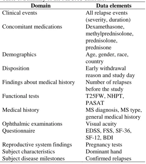
MS is a cell-mediated autoimmune condition in which episodes of inflammation of the nervous tissue in the spinal cord and brain occurs repeatedly [4]. The multiple scar tissue (sclerosis) along the neurons blocks or slows the signal transmission between the brain and spinal cord which causes impaired movement and sensation [4]. Fig. 1 depicts the MS attack on the central nervous system.
[image:1.595.308.537.148.386.2]Currently, MS has been classified into quite a few subtypes based on the clinical course (relapsing vs. progressive) and phenotype (e.g. benign or malignant) [5]. Severity classification of MS disease is necessary for treatment and medication dosage decisions and to understand the disease progression. Although this disease is common, clinicians find difficulty in assessing the severity, due to paucity of the organized data and nature of the disease. Therefore, this study may be helpful for the clinicians to assess the severity of MS patients and to take medication and dosage decisions.
Fig. 1. MS attack on the central nervous system (Source: neurologicalwellness.com)
The National multiple sclerosis society (NMSS) developed a task force to recommend outcome assessment methods [6]. They recommended quantitative neurological performance testing such as Timed 25-foot walk (T25FW), Nine-hole peg test (NHPT), Paced auditory serial addition test (PASAT) and urge to include the visual function test. The MSOAC recognized that outcome measures such as T25FW, 9HPT, and low contrast letter acuity can be used to classify the MS severity [7]. Reliability and validity of the metric considered as the outcome measure for the clinical trial and research project are essential [8]. According to T Jock Murray, the T25FW which is an MSOAC metric of walking was recognized as the central feature of MS [9]. Sandroff et al. [10] suggested the need for further research to interpret the importance of T25FW scores to understand its clinical and research relevance in MS.
NHPT has been proposed by MSOAC to measure the upper extremity function which is currently considered as the gold standard [11]. Lamers et al. [12] and Drake et al. [13] have shown that the NHPT distinguishes manual dexterity in MS subjects and healthy controls with high significant level (p < 0.05).
PASAT is a metric to measure the cognitive processing speed [14]. Loss of low-contrast vision is an important contributor to impairment and disability in MS [15].
Fig. 2. Symptoms of MS in different parts of the body (Source: healthline.com)
The RS approach provides numerous advantages in dealing with the imperfect knowledge (e.g. uncertainty, vagueness, ambiguity, imprecision, inconsistency, and incompleteness) over other approaches: (i) does not require any supplementary or prior information about the data like the grade of membership in fuzzy set theory and probability in statistics, (ii) the ability to reduce the original dataset into a minimal dataset which has the same knowledge as the original dataset, (iii) provides the facility to find the set of significant attributes and single most significant attributes, and (iv) ability to generate decision rules from the reduced dataset [16].
The RS-based approach is found to perform better than ML classifiers on many medical datasets. For instance, authors of [17] applied the RS-based approach on the five benchmark medical datasets (diabetes, heart disease, breast cancer, liver disorder, and hepatitis) acquired from the University of California at Irvine. They found that the RS-based approach outperformed the ML classifiers such as K-NN, SVM, Multilayer perceptron, and backpropagation algorithm. The RS-based approach has been applied for various tasks such as pattern recognition and classification [18], medical image processing [19], and massive data processing such as gene expression [20].
To the best of authors’ knowledge, until now no study has been done to classify the severity of MS disease. In this paper, the RS approach has been used for the severity classification of MS disease using the metrics that have a significant impact on the MS disease severity. The rest of the paper is organized as follows. Section II describes the rough set theory in detail. Section III gives a description of the dataset used for the MS disease severity classification. Section IV presents the methodology used for implementing the RS approach. Section V presents the results. Section VI concludes the paper.
II. ROUGH SET THEORY
Rough set theory (RST) was proposed by Pawlak in 1982, has the ability to deal with vagueness, imprecision, uncertainty, inconsistency, and incomplete data [21, 22]. The theory works in two stages. In the first stage, the rule is generated by classifying the relational database. In the second stage, knowledge is discovered through the classification of an equivalence relation. RST is a relatively new and effective intelligent information processing paradigm which was introduced after the probability theory, fuzzy set theory and evidence theory. In fuzzy set theory (FST) approach, the main problem is to assign the membership value which is uncertain. However, in the RST approach, the imprecise concepts are described by precise boundary lines (upper and lower approximation). Therefore, in a sense, for solving the uncertain problem the RST is certain whereas FST is uncertain [23].
In RST, instead of assigning the membership value to each of the elements of the set, the interest lies in using the available information about the elements to discern an element or a group of elements from the others. So, two distinct elements can be indistinguishable (indiscernible) on the basis of available information. For example, two acids having pK value 4.4 and 4.6 is considered equally weak and put together in the rough set ‘weak acid’ as compared to other relevant categories of classification (‘medium acid’ or ‘strong acid’) [24]. These acids are indistinguishable with respect to pK value.
The set of all indistinguishable (similar) elements are called elementary sets that form the basic ‘granule’ of knowledge. Union of the elementary sets is called precise sets. In the RS approach, boundary-line cases occur when the available information is not sufficient to classify the element with certainty into the member of the set or its complement. Two precise sets, namely, the lower and upper approximation, are associated with the rough set. The element which surely belongs to the set lies in the lower approximation. However, the elements which possibly belongs to the set lies in the upper approximation [25]. The concept of lower and upper approximation has been illustrated in Fig. 3.
[image:2.595.302.544.569.832.2]A. Preliminaries of Rough Set Theory
This section presents some basic notions related to the information system and rough set.
Definition 1. Information system [26]
An information system or an approximation space is
represented as 4-tuple where
is the finite set of objects and
is a finite nonempty set of attributes (features/variables) whose subsets and are condition attribute set and decision attribute set respectively. And where is the set of values of attribute , called the domain of attribute . Each attribute , defines an information
function, given by .
Definition 2. Indiscernibility relation [26]
Given a subset of attribute set , an indiscernible relation on the universe can be defined as follows.
(1)
Indiscernible relation is an equivalence relation. The equivalence class of an object is denoted by or
.
Definition 3. Upper and lower approximation sets [26]
Given an information system, for a
subset , the lower and upper approximation is defined as follows.
(2)
(3)
where denotes the equivalence class of x.
The family of all equivalence classes (quotient set of ) is
denoted by . The universe can be divided into
three disjoint regions, viz. positive, negative and boundary regions as follows.
(4)
(5)
(6)
Definition 4. Definable sets
Given an information system, for any
target subset and attribute subset , is said to
be definable set with respect to , iff .
Definition 5. Rough sets
Given an information system, for any
target subset and attribute subset , is said to
be rough set with respect to , iff .
The boundary region causes uncertainty in the rough set. The degree of uncertainty increases with increase in the boundary region. The metric used to measure the uncertainty of a rough set is roughness.
Definition 6. Roughness of a rough set
Given an information system, for any
target subset and attribute subset , the
roughness of set with respect to is defined as follows.
(7)
where
X
and denotes the cardinality of a finite set. The rough set theory comes under soft computing (SC) paradigm. SC paradigm has the ability to tolerate imprecision, vagueness, and uncertainty to find the approximate solution instead of an exact solution. So, the low-cost robust solution can be found for some real problems [27].Definition 7. Accuracy of approximation
The accuracy of the set in , is given by:
(8)
It can be easily observed that .
If X is definable in U. If X is undefinable in U.
Definition 8. Independence of attributes
To check whether the set of attributes is independent or not, every attribute has to be checked to find whether the removal of that attribute increases the number of elementary sets in the information system or not.
If
ind
(A)
ind
(A
a
i)
, then the attributea
iis said tobe superfluous. Otherwise, the attribute
a
iis indispensable inA
.Definition 9. Core and reduct of attributes
In case of the dependent set of attributes, determining all possible minimal subsets of attributes, which will have the same number of elementary sets as the whole set of attributes (reducts) is very crucial from the information processing point of view. Because this allows working with a smaller set of attributes that results in performance enhancement. Determining the set of all indispensable attributes (core) is also of particular interest as it tells about the most significant single attributes.
III. MSOACPLACEBO DATABASE
MSOAC Placebo database was obtained by the approval of MSOAC review board. The MS clinical trial database contains 2465 records which include data from many domains. The clinical events domain has information about the severity and duration of the MS disease. In concomitant medication domain, the attributes were the medicines prescribed to the subjects. The demographics domain has four attributes: age, gender, race, and country. The findings about medical history domain list
has four important attributes which are used to measure the extent of MS-disability such as T25FW, NHPT, and PASAT. The ophthalmic examinations domain has information about visual acuity. The questionnaires domain contains an expanded disability status scale (EDSS), functional systems scores (FSS), short form-36 (SF-36), short form-12 (SF-12), and beck depression inventory (BDI). The different data elements that belong to each domain has been summarized in Table 1.
Table 1. Summary of the MSOAC database.
Domain Data elements
Clinical events All relapse events
(severity, duration)
Concomitant medications Dexamethasone,
methylprednisolone, prednisolone, prednisone
Demographics Age, gender, race,
country
Disposition Early withdrawal
reason and study day Findings about medical history Number of relapses
before the study
Functional tests T25FW, NHPT,
PASAT
Medical history MS diagnosis, MS type,
general medical history Ophthalmic examinations Visual acuity
Questionnaire EDSS, FSS, SF-36,
SF-12, BDI Reproductive system findings Pregnancy tests
Subject characteristics Dominant hand
Subject disease milestones Confirmed relapses
IV. THE METHODOLOGY USED FOR IMPLEMENTING A ROUGH SET APPROACH
A. Preparation of Datasets
The MSOAC Placebo database has some missing value, therefore, the original MSOAC database is used to prepare the two datasets (dataset A and dataset B) by using the attribute selection and pre-processing steps discussed below.
The dataset A contains no missing value whereas dataset B is allowed to have some missing value. Both the datasets are imbalanced. However, dataset B allows some missing value to alleviate data imbalance.
The dataset A contains the details of 472 patients in which there is no missing value. But the problem with this dataset is that it is highly imbalanced as the severe cases are very poorly represented in the dataset. It contains 39%, 48%, and 11% respectively the mild, moderate, and severe cases.
Dataset B is prepared to alleviate the data imbalance. This dataset contains the details of 898 patients with some missing value. In this dataset, the representation of mild, moderate, and severe cases is 35%, 50%, and 15% respectively. Here, the representation of severe case is increased from 11% to 15%. In order to complete the dataset B, mean/mode imputation technique is used. Fig. 4 shows the workflow of MS severity classification using the RS approach.
B. Attribute Selection
[image:4.595.315.534.203.328.2]The attributes are selected manually by considering the recommendations of the NMSS, MSOAC, and authors of various studies on the MS disease. This includes NHPT, T25FW, PASAT, T25FW, and Visual acuity (VA). The other attributes such as age, gender, and the number of relapses (NoR) are also considered because these attributes may influence the severity of the MS disease. The selected decision and conditional attributes are listed in Table 2. The information system is developed which has seven conditional attributes and a decision attribute.
Table 2. Attributes in datasets A & B.
Sl. No. Attributes Attribute Type
1
Age Conditional2
Gender Conditional3
Number of relapses Conditional4
NHPT Conditional5
PASAT Conditional6
T25FW Conditional7
Visual acuity Conditional8
Severity DecisionC. Pre-processing
As MSOAC data is a clinical trial data, therefore, functional tests (NHPT, PASAT, T25FW, and VA) have been done more than once for the same patient during different visits. In order to take single value for each of the tests, the mean of all the value for a particular test was calculated for each patient. The attribute value of NoR is added cumulatively for each patient till the last visit to get the final value.
D. Discretization
As the values for some attributes are continuous, therefore, the final dataset needs to be discretized. The discretization process saves the processing time and improves the quality of the result. More general decision rules can be obtained by using scaled attributes. The semi-naïve bayes discretization technique has been used to discretize the final dataset.
E. Data Split
After the data pre-processing, both the datasets are split into training and testing set in which the training set consists of 70% of records and test set consists of 30% of records.
F. Reduction
This process is conducted to spot the minimal attributes that represent knowledge patterns in the data. Finding all reduct is an NP-complete problem [28]. Therefore, approximation algorithms such as Johnson’s [29] and Genetic algorithms [30] have been used for the generation of reduct. The reduct set is generated by constructing the discernibility function. The decisions rules are generated from these reduct set. Sometimes decision rules generated by using the RS approach are not acceptable. This happens when there is a relatively small number of examples that supports the rule. After the decision rule set is computed, the conflict between the decision rules needs to be
classify the objects into different decision classes.
G. Johnson’s Algorithm
Johnson’s algorithm (JA) generates only a single reduct with the minimum number of attributes. The algorithm selects the attribute which appears the maximum number of times in each iteration. JA, first set the value of S, the current reduct candidate, to an empty set. After that, the algorithm counts the number of times each attribute occurs in the clause. The attribute which has the highest count is added into S, and all clauses in f comprising this attribute are excluded from the discernibility function. This process iterates until all clauses are removed from the discernibility function. Finally, the algorithm returns S as a reduct.
Seven reducts generated by JA are: {Age}, {T25FW}, {NHPT}, {PASAT}, {NoR}, {Age, NoR} and {Age, T25FW}. This means all these attribute set play an important role in classifying the severity level in MS disease. However, each of these attributes has support value 100, therefore, their importance in classification seems to be equal.
H. Genetic Algorithm
Genetic algorithm (GA) is an efficient method to compute the reduct set. It gives a good approximation. The idea of GA is based on the Darwinian principle “survival of the fittest” (natural selection). In a classical genetic algorithm, a state space S and a function are given.
+
And, the goal is to find
Elements of set S are “individuals”. The value of function is a measure of the ability to survive in the environment, called “fitness”. The evolution process can be simulated as follows [31].
1. A representation scheme is chosen to map space of “individuals” into “chromosomes” which is usually a bit string.
2.Set of chromosomes is chosen randomly as the initial population.
3.The “fitness” of each chromosome is calculated as the value where is the individual encoded by . After that, the new population is created by replacing the chromosomes having low fitness value by those with higher fitness. 4. Now, the genetic operators such as mutation and
crossing-over are applied randomly on the new population. The mutation causes small random
modification in the chromosomes while
crossing-over takes place by the exchange of “genetic material” between some pairs of chromosomes.
5. The steps 3-4 is repeated with the new population until a stopping criterion is satisfied.
Usually, the classical GA generates 5 to 50 numbers of reducts. Reducts that generates less number of rules is desirable as these rules are more general and can better recognize new cases [32].
Genetic algorithm generated 39 reducts with dataset A and 75 reducts with dataset B. The reducts set contains all the individual attributes and their combination.
I. Decision Rules
The decision rules have two parts. The part is called the premise or the antecedent and the part is called the consequent. In order to form the rules, each attribute of the reduct reads one or more values and associate them with one or more decision classes. For example, suppose the reduct set has two attributes, say, { } where reads the value and read the value. Now, the rule
can be associated with the corresponding decision class. For two-class classification, the decision classes can be or . The rule could be:
or
.
The part includes only one decision class unless the decision class is rough with regard to the attribute in the reduct. The rules should be general and specific. The generality of the rule is evaluated by the metric coverage, which refers to the fraction of objects from the decision class in the part that also matches with the part. How specific a rule is measured by accuracy, which corresponds to the fraction of objects matching the part that is from the decision class of part [33].
The decision rules generated by both the JA and GA have very poor coverage. This is because the naïve bayes discretization technique discretized the attributes into very small intervals. In such cases, rules become highly specific. Specific rules are usually large in numbers. We have 933 rules using the GA and 232 rules using JA on dataset A. The number of rules will become even larger on dataset B.
J. Classification
Fig. 4. The workflow of MS severity classification using the rough set approach
V. RESULTS
The proposed rough set approach was trained on PC workstation with two core Intel i5 2.5 GHz processors and 8GB of RAM. The performance of the RS approach and ML classifiers is evaluated on the dataset A and dataset B. For the implementation of ML classifiers, the same datasets (dataset A and dataset B) are used which is obtained after the attribute selection and pre-processing. It must be noted that for ML implementation, the datasets are not discretized because discretization may reduce the performance of ML classifiers. The classifiers (RF, K-NN, and SVM) are tuned to get the best performance in terms of accuracy, precision, recall, and specificity. The best values of the performance metrics are found when both the datasets A and B is split in the ratio of 80/20.
In the RS implementation, the reduction algorithm is applied to the training set of the datasets and it is found that the performance of GA is better than JA. These algorithms generate the rules which are used to classify the test set. Now, we have used standard voting (SV) and voting with object tracking (VWOT) as the classification algorithms. For our datasets, VWOT algorithm performed better than SV in classifying the severity of the MS disease.
The confusion matrixes for dataset A and dataset B (in case of RS approach) is presented in Table 3 and 5 respectively. These confusion matrixes are obtained by applying GA and VWOT as the reduction and classification algorithms respectively. It can be observed from Table 3 that out of 59 mild cases, 18.64% and 13.55% cases are wrongly classified into moderate and severe cases. Similarly, out of 70 moderate cases respectively, only 2.85% and 1.42% are wrongly classified into mild and severe. Likewise, out of 12 severe cases, 16.66% and 66.66% cases are wrongly classified as mild and moderate respectively. Misclassification rate for the severe case is unacceptably high. Also, it can be observed from Table 5 that out of 104 mild cases, 25.96% and 12.50%
cases are misclassified into moderate and severe respectively. Likewise, out of 126 moderate cases, 9.52% and 5.55% cases are wrongly classified as mild and severe respectively. Similarly, out of 37 severe cases, 18.91% and 27.02% cases are misclassified into mild and moderate respectively.
Table 3. A confusion matrix for dataset A in the RS approach. Predicted
Mild Moderate Severe Original Mild 40 11 8
Moderate 2 67 1 Severe 3 8 2
Table 4. Classification performance of RS approach with dataset A.
Class acc (%) prec (%) recall (%) spec (%) Mild
Moderate Severe
83.09 88.88 67.79 93.97
84.50 77.90 95.71 73.61
[image:6.595.81.259.49.313.2]85.91 18.18 15.38 93.02
Table 5. A confusion matrix for dataset B in the RS approach. Predicted
Mild Moderate Severe Original Mild 66 27 13
Moderate 12 107 7 Severe 7 10 20
Table 6. Classification performance of RS approach with dataset B.
Class acc (%) prec (%) recall (%) spec (%) Mild
Moderate Severe
83.09 88.88 67.79 93.97
84.50 77.90 95.71 73.61
85.91 18.18 15.38 93.02
Furthermore, the precision values for each class (mild, moderate and severe) are recorded in Tables 4 and 6. In Table 4, the precision for the mild, moderate, and severe classes are 88.88%, 77.90%, and 18.18% respectively. This shows that the probability of correctly detecting the mild class is higher than moderate and severe classes and that the probability of correctly detecting the severe class is lowest. Similarly, in Table 6, the precision for the mild, moderate, and severe classes are 77.64%, 74.30%, and 50% respectively. This again shows that the probability of correctly identifying the mild class is highest and the probability of correctly identifying the severe class is lowest. This also verifies the consistency of the two datasets.
The overall (weighted average) performance of the RS approach and different ML classifiers are listed in Table 7. It can be observed from this table that RS approach which is implemented on dataset A is the most efficient in terms of all the performance metrics. This is because dataset A has no missing value and also RS approaches does not require large dataset. But due to highly imbalanced dataset (out of a total of 142 test dataset only 13 belongs to severe class), the precision and recall values are very low. This prompted us to prepare another dataset B that allows some missing value. The precision and recall for
[image:6.595.301.552.410.458.2]dataset B, the precision and recall become 50% and 54.05% respectively, but the overall performance is better with the dataset A. The weighted average accuracy, precision, recall, and specificity values for dataset A are 84.04%, 76.99%, 76.75%, and 83.84% respectively. The RS approach on both the datasets performed much better than ML classifiers. Among the ML classifiers, the performance of random forest classifier is found best for which the weighted average accuracy, precision, recall, and specificity values are 62.19 %, 52.65 %, 56.84 %, and 59.87 % respectively with dataset A.
Table 7. Weighted average performance.
Algorithms Dataset used acc
(%) prec (%) recall (%) spec (%)
Rough set Dataset A 84.04 76.99 76.75 83.84
RF Dataset A 62.19 52.65 56.84 59.87
K-NN Dataset A 51.08 45.72 44.21 52.18
SVM Dataset A 52.49 44.56 46.32 51.45
Rough set Dataset B 79.70 72.27 71.74 82.09
RF Dataset B 56.23 45.16 48.33 52.10
K-NN Dataset B 55.62 40.65 47.78 50.09
SVM Dataset B 59.72 44.70 52.78 45.66
[image:7.595.42.292.422.614.2]In Table 8, we have shown the weighted average performance of different reduction and classification approach used in the RS-based framework. With dataset A, genetic and VWOT is the best reduction and classification algorithms respectively. However, precision with the Johnson algorithm is better but the recall is low. The same happens with the dataset B.
Table 8. Weighted average performance in the rough set approach. Reductio n Algorith m Classificatio n Algorithm Datase t used acc (%) prec (%) recall (%) spec (%)
Genetic SV A 83.68 76.7
5
76.0 5
83.7 7
Genetic VWOT A 84.04 76.9
9
76.7 5
83.8 4
Johnson SV A 79.65 91.4
8
62.6 7
95.6 2
Johnson VWOT A 79.65 91.4
8
62.6 7
95.6 2
Genetic SV B 78.10 70.2
6
69.8 8
80.7 1
Genetic VWOT B 79.70 72.2
7
71.7 4
82.0 9
Johnson SV B 76.30 70.2
6
69.8 8
92.0 9
Johnson VWOT B 76.30 85.3
0
58.7 3
92.0 6
It is important to note that in both Tables 5 and 6, the class weighted average performance is considered. This is because, in case of highly imbalanced datasets, the class weighted average performance can provide better insight about the classification performance.
VI. CONCLUSION
The paper proposed a rough set approach to classifying the severity level of Multiple Sclerosis disease. The performance of the rough set approach was compared with ML classifiers. The weighted average accuracy, precision, recall, and specificity values for the rough set approach were found to be 84.04%, 76.99%, 76.75%, and 83.84% respectively.
However, among the ML classifiers, the performance of random forest classifier was found best for which the weighted average accuracy, precision, recall, and specificity values were 62.19 %, 52.65 %, 56.84 %, and 59.87 % respectively. The rough set approach is found much superior to ML classifiers. This study may be helpful for the clinicians to assess the severity of the MS patients and to take medication and dosage decisions. In the future, we would like to add some more attributes from different domains. The effect of genomic factors may also be included to understand the MS severity in a personalized manner.
CONFLICT OF INTEREST There is no conflict of interest in this work.
ACKNOWLEDGMENT
Data used in the preparation of this article were obtained from the Multiple Sclerosis Outcome Assessments Consortium (MSOAC). As such, the investigators within MSOAC contributed to the design and implementation of the MSOAC Placebo database and/or provided placebo data, but did not participate in the analysis of the data or the writing of this report.
The authors would also like to acknowledge the Ministry of Electronics & Information Technology (MeitY), Government of India for supporting the research work through “Visvesvaraya Ph. D. Scheme for Electronics & IT”.
REFERENCES
[1]Browne, P., et al., Atlas of multiple sclerosis 2013: a growing global problem with widespread inequity. Neurology, 2014. 83(11): p. 1022-1024.
[2]Federation, M.S.I., Atlas of MS 2013: Mapping multiple sclerosis around
the world. Mult Scler Int Fed, 2013: p. 1-28.
[3]Mackenzie, I., et al., Incidence and prevalence of multiple sclerosis in the UK 1990–2010: a descriptive study in the General Practice Research Database. J Neurol Neurosurg Psychiatry, 2014. 85(1): p. 76-84.
[4]Johnston Jr, R.B. and J.E. Joy, Multiple sclerosis: current status and strategies for the future. 2001: National Academies Press.
[5]Lublin, F.D., et al., Defining the clinical course of multiple sclerosis: the 2013 revisions. Neurology, 2014. 83(3): p. 278-286.
[6]Whitaker, J., et al., Outcomes assessment in multiple sclerosis clinical trials: a critical analysis. Multiple Sclerosis Journal, 1995. 1(1): p. 37-47.
[7]LaRocca, N.G., et al., The MSOAC approach to developing performance
outcomes to measure and monitor multiple sclerosis disability. Multiple Sclerosis Journal, 2018. 24(11): p. 1469-1484.
[8]Cohen, J.A., et al., Disability outcome measures in multiple sclerosis clinical trials: current status and future prospects. The Lancet Neurology, 2012. 11(5): p. 467-476.
[9]T Jock Murray, M., Multiple sclerosis: the history of a disease. 2004: Demos medical publishing.
[10] Sandroff, B.M., et al., Further validation of the Six-Spot Step Test as a measure of ambulation in multiple sclerosis. Gait & posture, 2015. 41(1): p. 222-227.
[11] Hulst, H.E., A.J. Thompson, and J.J. Geurts, The measure tells the tale: Clinical outcome measures in multiple sclerosis. 2017, SAGE Publications Sage UK: London, England.
[12] Lamers, I., et al., Perceived and actual arm performance in multiple
sclerosis: relationship with clinical tests according to hand dominance. Multiple Sclerosis Journal, 2013. 19(10): p. 1341-1348.
[13] Drake, A., et al., Psychometrics and normative data for the Multiple
Sclerosis Functional Composite: replacing the PASAT with the Symbol Digit Modalities Test.
Multiple Sclerosis Journal, 2010. 16(2): p. 228-237. [14] Rudick, R., et al., Clinical
Author-2 Photo
multiple sclerosis. Annals of Neurology: Official Journal of the American Neurological Association and the Child Neurology Society, 1996. 40(3): p. 469-479.
[15] Balcer, L.J., et al., Validity of low-contrast letter acuity as a visual performance outcome measure for multiple sclerosis. Multiple Sclerosis Journal, 2017. 23(5): p. 734-747.
[16] Suraj, Z., An introduction to rough set theory and its applications. ICENCO, Cairo, Egypt, 2004. 3: p. 80.
[17] Inbarani, H.H., A novel neighborhood rough set based classification
approach for medical diagnosis. Procedia Computer Science, 2015. 47: p. 351-359.
[18] Nyirarugira, C. and T. Kim, Stratified gesture recognition using the normalized longest common subsequence with rough sets. Signal Processing: Image Communication, 2015. 30: p. 178-189.
[19] Hassanien, A.E., et al., Rough sets in medical imaging: foundations and trends, in Computational Intelligence in Medical Imaging. 2009, Chapman and Hall/CRC. p. 61-102.
[20] Wabnik, K., et al., Gene expression trends and protein features
effectively complement each other in gene function prediction. Bioinformatics, 2008. 25(3): p. 322-330.
[21] Pawlak, Z., Rough sets. International journal of computer &
information sciences, 1982. 11(5): p. 341-356.
[22] Pawlak, Z., Rough sets: Theoretical aspects of reasoning about data.
Vol. 9. 2012: Springer Science & Business Media.
[23] Zhang, Q., Q. Xie, and G. Wang, A survey on rough set theory and its
applications. CAAI Transactions on Intelligence Technology, 2016. 1(4): p. 323-333.
[24] Walczak, B. and D. Massart, Rough sets theory. Chemometrics and
intelligent laboratory systems, 1999. 47(1): p. 1-16.
[25] Pawlak, Z., Rough set theory and its applications to data analysis. Cybernetics & Systems, 1998. 29(7): p. 661-688.
[26] Pawlak, Z., et al., Rough sets. Communications of the ACM, 1995. 38(11): p. 88-95.
[27] Ross, T.J., Fuzzy logic with engineering applications. Vol. 2. 2004: Wiley Online Library.
[28] Skowron, A. and C. Rauszer, The discernibility matrices and functions
in information systems, in Intelligent decision support. 1992, Springer. p. 331-362.
[29] Johnson, D.S., Approximation algorithms for combinatorial
problems. Journal of computer and system sciences, 1974. 9(3): p. 256-278.
[30] Vinterbo, S. and A. Øhrn, Minimal approximate hitting sets and rule
templates. International Journal of approximate reasoning, 2000. 25(2): p. 123-143.
[31] Goldberg, D.E. and J.H. Holland, Genetic algorithms and machine
learning. Machine learning, 1988. 3(2): p. 95-99.
[32] Bazan, J.G., et al., Rough set algorithms in classification problem, in
Rough set methods and applications. 2000, Springer. p. 49-88.
[33] Hvidsten, T.R., A tutorial-based guide to the ROSETTA system: A
Rough Set Toolkit for Analysis of Data. 2010.
AUTHORSPROFILE
Afzal Hussain Shahid received his B. Tech. degree in Computer Science and Engineering from Netaji Subhash Engineering College (Garia, Kolkata) in 2010. He received his M.Tech. degree in Computer Science and Engineering from NIT Patna (Patna, Bihar) in 2013. He now works as a Research Scholar at NIT Patna. His area of research is Machine Learning.
Dr. M. P. Singh received his Ph.D. degree in Computer Science and Engineering from Motilal Nehru National Institute of Technology Allahabad (Uttar Pradesh) in 2008. He is currently working as an Associate Professor with the Department of Computer Science and Engineering in National Institute of Technology Patna. His research area includes Social Media, Wireless Sensor Networks, Fuzzy set, E-learning, Ad hoc network, Database System and Semantic Web.
Dr. Gunjan Kumar received his MD degree in Medicine from Dr. Ram Manohar Lohia Hospital and Post Graduate Institute of Medical Education and Research (New Delhi) in 2012. He received his DM