High Performance Multidimensional Scaling for Large High Dimensional Data Visualization

High Performance Multidimensional Scaling

for Large High-Dimensional Data Visualization

Seung-Hee Bae, Judy Qiu, Member, IEEE, and Geoffrey Fox, Member, IEEE

Abstract—Technical advancements produces a huge amount of scientific data which are usually in high dimensional formats, and it is getting more important to analyze those large-scale high-dimensional data. Dimension reduction is a well-known approach for high-dimensional data visualization, but can be very time and memory demanding for large problems. Among many dimension reduction methods, multidimensional scaling does not require explicit vector representation but uses pair-wise dissimilarities of data, so that it has a broader applicability than the other algorithms which can handle only vector representation. In this paper, we propose an efficient parallel implementation of a well-known multidimensional scaling algorithm, called SMACOF (Scaling by MAjorizing a COmplicated Function) which is time and memory consuming with a quadratic complexity, via a Message Passing Interface (MPI). We have achieved load balancing in the proposed parallel SMACOF implementation which results in high efficiency. The proposed parallel SMACOF implementation shows the efficient parallel performance through the experimental results, and it increases the computing capacity of the SMACOF algorithm to several hundreds of thousands of data via using a 32-node cluster system.

Index Terms—Multidimensional scaling, Parallelism, Distributed applications, Data visualization.

✦

1

I

Due to the innovative advancements in science and technology, the amount of data to be processed or analyzed is rapidly growing and it is already beyond the capacity of most commodity hardware we are us-ing currently. To keep up with such fast development, study for data-intensive scientific data analyses [1] has been already emerging in recent years. It is a challenge for various computing research communities, such as high-performance computing, database, and machine learning and data mining communities, to learn how to deal with such large and high dimensional data in this data deluged era. Unless developed and imple-mented carefully to overcome such limits, techniques will face soon the limits of usability. Parallelism is not an optional technology any more but an essential factor for various data mining algorithms, including dimension reduction algorithms, by the result of the enormous size of the data to be dealt by those algo-rithms (especially since the data size keeps increas-ing).

Visualization of high-dimensional data in low-dimensional space is an essential tool for exploratory data analysis, when people try to discover meaningful information which is concealed by the inherent com-plexity of the data, a characteristic which is mainly dependent on the high dimensionality of the data. That is why the dimension reduction algorithms are highly used to do a visualization of high-dimensional

• S.-H. Bae, J. Qiu and G. Fox are with the Pervasive Technology Institute, Indiana University, Bloomington, IN, 47408.

Email: [email protected],xqiu,[email protected]

data. Among several kinds of dimension reduction algorithms, such as Principle Component Analysis (PCA), Generative Topographic Mapping (GTM) [2], [3], Self-Organizing Map (SOM) [4], Multidimensional Scaling (MDS) [5]–[7], to name a few, we focus on the MDS in our paper due to its wide applicability and theoretical robustness.

The task of visualizing high-dimensional data is getting more difficult and challenged by the huge amount of the given data. In most data analysis with such large and high-dimensional dataset, we have observed that such a task is not only CPU bounded but also memory bounded, in that any single process or machine cannot hold the whole data in its memory any longer. In this paper, we tackle this problem for developing a high performance visualization for large and high-dimensional data analysis by using distributed resources with parallel computation. For this purpose, we will show how we developed a well-known MDS algorithm, which is a useful tool for data visualization, in a distributed fashion so that one can utilize distributed memories and be able to process large and high dimensional datasets.

This paper is an extended version of [8], and this paper shows a slight update of parallel

implemen-tation and more experimental analyses in detail. 1

In Section 2, we provide an overview of what the mul-tidimensional scaling (MDS) is, and briefly introduce a well-known MDS algorithm, named SMACOF [9], [10] (Scaling by MAjorizing a COmplicated Function). We explain the details of the proposed parallelized

version of the SMACOF algorithm, called parallel SMACOF, in Section 3. In the next, we show our performance results of our parallel version of MDS in various compute cluster settings, and we present the results of processing up to 100,000 data points in Section 4 followed by the related work in Section 5. We summarize the conclusion and future works of this paper in Section 6.

2

M

S

(MDS)

Multidimensional scaling (MDS) [5]–[7] is a general term that refers to techniques for constructing a map of generally high-dimensional data into a target di-mension (typically a low didi-mension) with respect to the given pairwise proximity information. Mostly, MDS is used to visualize given high dimensional data or abstract data by generating a configuration of the given data which utilizes Euclidean low-dimensional space, i.e. two-dimension or three-dimension.

Generally, proximity information, which is

repre-sented as an N ×N dissimilarity matrix (∆= [δij]),

where N is the number of points (objects) and δij

is the dissimilarity between point i and j, is given

for the MDS problem, and the dissimilarity matrix

(∆) should agree with the following constraints: (1)

symmetricity (δij = δji), (2) nonnegativity (δij ≥ 0),

and (3) zero diagonal elements (δii= 0).

The objective of the MDS technique is to construct a configuration of a given high-dimensional data into low-dimensional Euclidean space, where each dis-tance between a pair of points in the configuration is approximated to the corresponding dissimilarity value as much as possible. The output of MDS

algo-rithms could be represented as anN×Lconfiguration

matrix X_{, whose rows represent each data point xi}

(i = 1, . . . , N) in L-dimensional space. It is quite straightforward to compute the Euclidean distance

between xi and xj in the configuration matrix X,

i.e. dij(X) = kxi−xjk, and we are able to evaluate

how well the given points are configured in the L

-dimensional space by using the suggested objective functions of MDS, called STRESS [11] or SSTRESS [12]. Definitions of STRESS (1) and SSTRESS (2) are follow-ing:

σ(X_{) =} X

i<j≤N

wij(dij(X)−δij)2 (1)

σ2(X_{) =} X

i<j≤N

wij[(dij(X))2−(δij)2]2 (2)

where 1 ≤i < j ≤ N and wij is a weight value, so

wij≥0.

As shown in the STRESS and SSTRESS functions, the MDS problems could be considered to be non-linear optimization problems, which minimizes the STRESS or the SSTRESS function in the process of

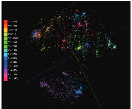
Fig. 1. An example of the data visualization of 30,000 biological sequences by an MDS algorithm, which is colored by a clustering algorithm.

configuring an L-dimensional mapping of the

high-dimensional data.

Fig. 1 is an example of the data visualization of 30,000 biological sequence data, which is related to a metagenomics study, by an MDS algorithm, named SMACOF [9], [10] explained in Section 2.1. The colors of the points in Fig. 1 represent the clusters of the data, which is generated by a pairwise clustering algorithm by deterministic annealing [13]. The data visualization in Fig. 1 shows the value of the di-mension reduction algorithms which produced lower dimensional mapping for the given data. We can see clearly the clusters without quantifying the quality of the clustering methods statistically.

2.1 SMACOF and its Complexity

There are a lot of different algorithms which could be used to solve the MDS problem, and Scaling by MAjorizing a COmplicated Function (SMACOF) [9], [10] is one of them. SMACOF is an iterative ma-jorization algorithm used to solve the MDS problem with the STRESS criterion. The iterative majorization procedure of the SMACOF could be thought of as an Expectation-Maximization (EM) [14] approach. Al-though SMACOF has a tendency to find local minima due to its hill-climbing attribute, it is still a powerful method since the algorithm, theoretically, guarantees

a decrease in the STRESS (σ) criterion monotonically.

Instead of a mathematically detail explanation of the SMACOF algorithm, we illustrate the SMACOF pro-cedure in this section. For the mathematical details of the SMACOF algorithm, please refer to [7].

Algorithm 1SMACOF algorithm

1: Z_⇐X[0]_; 2: k⇐0;

3: ε⇐small positive number;

4: M AX⇐ maximum iteration;

5: Compute σ[0]_=σ(X[0]_);

6: while k= 0 or (∆σ > εand k≤M AX)do

7: k⇐k+ 1;

8: X[k]₌V†B₍X[k−1]₎X[k−1] 9: Compute σ[k]_=σ(X[k]₎

10: Z_⇐X[k]_; 11: end while 12: return Z_;

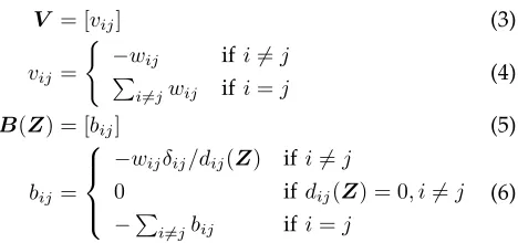
V†_{is the Moore-Penrose inverse [15], [16] (or}

pseudo-inverse) of matrixV_{. TheN×N matrices}V _andB₍Z₎

are defined as follows:

V _{= [vij] (3)}

vij = (

−wij if i6=j P

i6=jwij if i=j

(4)

B₍Z_{) = [bij] (5)}

bij =   

 

−wijδij/dij(Z) if i6=j

0 if dij(Z) = 0, i6=j

−P

i6=jbij if i=j

(6)

If the weights are equal to one (wij = 1) for all

pairwise dissimilarities, thenV _andV†_{are simplified}

as follows:

V _{= N}

I−ee

t

N

(7)

V† ₌ 1

N

I−ee

t

N

(8)

where e _{= (1, . . . ,1)}t _{is one vector whose length is}

N. In this paper, we generate mappings based on the

equal weights weighting scheme and we use (8) for

V†_.

As in Alg. 1, the computational complexity of the

SMACOF algorithm is O(N2_{), since the Guttman}

transform performs a multiplication of an N ×N

matrix and an N×L matrix twice, typically N ≫L

(L = 2 or 3), and the computation of the STRESS

value,B₍X[k]_{), and}D₍X[k]_{)also takeO(N}2_{). In}

addi-tion, the SMACOF algorithm requiresO(N2_)memory

because it needs severalN×Nmatrices, as in Table 1.

Due to the trends of digitization, data sizes have increased enormously, so it is critical that we are able to investigate large data sets. However, it is impossible to run SMACOF for a large data set under a typical single node computer due to the memory requirement

increases in O(N2_{). In order to remedy the shortage}

of memory in a single node, we illustrate how to

TABLE 1

Main matrices used in SMACOF

Matrix Size Description

∆ N×N Matrix for the given pairwise

dissimilar-ity[δij]

D₍X₎ N×N Matrix for the pairwise Euclidean

dis-tance of mappings in target dimension [dij]

V _N×_N Matrix defined by the value_vijin (3)

V† _{N×N Matrix for pseudo-inverse of}V B₍Z_{) N}×_{N Matrix defined by the valuebijin (5)}

W _N×N Matrix for the weight of the dissimilarity

[wij]

X[k] _{N×L Matrix for current L-dimensional} con-figuration of N data points x[k]

i (i =

1, . . . , N)

X[k−1] N×L Matrix for previousL-dimensional

con-figuration of N data points x[k−1]

i (i =

1, . . . , N)

parallelize the SMACOF algorithm via message pass-ing interface (MPI) for utilizpass-ing distributed-memory cluster systems in Section 3.

3

H

P

M

-SIONAL

S

We have observed that processing a very large dataset

is not only a cpu-bounded but also a memory-bounded

computation, in that memory consumption is beyond the ability of a single process or even a single machine, and that it will take an unacceptable running time to run a large data set even if the required memory is available in a single machine. Thus, running machine learning algorithms to process a large dataset, includ-ing MDS discussed in this paper, in a distributed fashion is crucial so that we can utilize multiple processes and distributed resources to handle very large data. The memory shortage problem becomes more obvious if the running OS is 32-bit which can handle at most 4GB virtual memory per process. To process large data with efficiency, we have developed a parallel version of the MDS by using a Message Passing Interface (MPI) fashion. In the following, we will discuss more details on how we decompose data used by the MDS algorithm to fit in the memory limit of a single process or machine. We will also discuss how to implement an MDS algorithm, called SMACOF, by using MPI primitives to get some com-putational benefits of parallel computing.

3.1 Parallel SMACOF

Table 1 describes frequently used matrices in the SMACOF algorithm. As shown in Table 1, the mem-ory requirement of the SMACOF algorithm increases

quadratically as N increases. For the small dataset,

large data set, such as hundreds of thousands or even

millions. For instance, ifN = 10,000, then oneN×N

matrix of 8-byte double-precision numbers consumes

800 MB of main memory, and if N = 100,000, then

one N×N matrix uses 80 GB of main memory. To

make matters worse, the SMACOF algorithm

gener-ally needs sixN×N matrices as described in Table 1,

so at least 480 GB of memory is required to run SMA-COF with 100,000 data points without considering

twoN×Lconfiguration matrices in Table 1 and some

required temporary buffers.

If the weight is uniform (wij= 1,∀i, j), we can use

only four constants for representing N ×N V _and

V† _{matrices in order to saving memory space. We,}

however, still need at least threeN×N matrices, i.e.

D₍X_{),∆, and}B₍X_{), which requires 240 GB memory}

for the above case, which is still an unfeasible amount of memory for a typical computer. That is why we have to implement a parallel version of SMACOF with MPI.

To parallelize SMACOF, it is essential to ensure load balanced data decomposition as much as possible. Load balance is important not only for memory distri-bution but also for computational distridistri-bution, since parallelization implicitly benefits computation as well as memory distribution, due to less computing per process. One simple approach of data decomposition

is that we assume p = n2_{, where p is the number}

of processes and n is an integer. Though it is a

relatively less complicated decomposition than others, one major problem of this approach is that it is a quite strict constraint to utilize available computing processors (or cores). In order to release that

con-straint, we decompose an N ×N matrix to m×n

block decomposition, wheremis the number of block

rows and nis the number of block columns, and the

only constraint of the decomposition is m×n = p,

where1≤m, n≤p. Thus, each process requires only

approximately 1/p of the full memory requirements

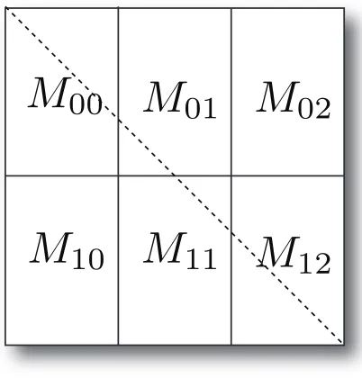
of SMACOF algorithm. Fig. 2 illustrates how we

decompose eachN×N matrix with 6 processes and

m= 2, n= 3. Without a loss of generality, we assume

N%m=N%n= 0 in Fig. 2.

A process Pk,0 ≤ k < p (sometimes, we will use

Pij for matching Mij) is assigned to one rectangular

blockMij with respect to the simple block assignment

equation in (9):

k=i×n+j (9)

where 0 ≤ i < m,0 ≤ j < n. For N ×N matrices,

such as ∆,V†_,B₍X[k]_{), and so on, each block Mij}

is assigned to the corresponding processPij, and for

X[k] _and X[k−1] matrices, N × L matrices where

L is the target dimension, each process has a full

N×Lmatrix because these matrices have a relatively

smaller size, and this results in reducing the number of additional message passing routine calls. By

scat-M

₀₀

_M

₀₁

_M

₀₂

M

₁₀

M

₁₁

_M

₁₂

Fig. 2. An example of anN×N matrix decomposition

of parallel SMACOF with 6 processes and2×3block

decomposition. Dashed line represents where diago-nal elements are.

Algorithm 2Pseudo-code for block row and column assignment for each process for high load balance.

Input: pNum, N, myRank

1: if N%pN um= 0 then

2: nRows = N / pNum;

3: else

4: if myRank≥(N%pN um)then

5: nRows = N / pNum;

6: else

7: nRows = N / pNum + 1;

8: end if

9: end if

10: return nRows;

tering decomposed blocks throughout the distributed memory, we are now able to run SMACOF with as huge a data set as the distributed memory will allow, via paying the cost of message passing overheads and a complicated implementation.

Although we assumeN%m =N%n= 0in Fig. 2,

there is always the possibility that N%m 6= 0 or

N%n 6= 0. In order to achieve a high load balance

under the N%m 6= 0 or N%n 6= 0 cases, we use a

simple modularoperation to allocate blocks to each

process with at most ONE row or column difference between them. The block assignment algorithm is illustrated in Alg. 2.

At the iterationk in Alg. 1, the application should

acquire up-to-date information of the following matri-ces:∆,V†_,B₍X[k−1]_),X[k−1]_{, andσ}[k]_{, to implement}

Line 8 and Line 9 in Alg. 1. One good feature of the SMACOF algorithm is that some of matrices are

x

=

M

M

M

M

M

M

M

X

X

X

C0

C1

C

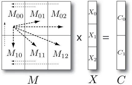
X

Fig. 3. Parallel matrix multiplication of N ×N matrix

andN×Lmatrix based on the decomposition of Fig. 2

the other hand, B₍X[k−1]_{) and STRESS (σ}[k]_{) value}

keep changing at each iteration, sinceX[k−1]_andX[k]

are changed in every iteration. In addition, in order to update B₍X[k−1]_{) and the STRESS (σ}[k]_{) value in}

each iteration, we have to take the N×N matrices’

information into account, so that related processes should communicate via MPI primitives to obtain the necessary information. Therefore, it is necessary to de-sign message passing schemes to do parallelization for calculating theB₍X[k−1]_{)and STRESS (σ}[k]_{) values as}

well as the parallel matrix multiplication in Line 8 in Alg. 1.

Computing the STRESS (Eq. (10)) can be

imple-mented simply by a partial error sum ofD_{ij and∆ij}

followed by anMPI_Allreduce:

σ(X_{) =} X

i<j≤N

wij(dij(X)−δij)2 (10)

where 1 ≤i < j ≤ N and wij is a weight value, so

wij≥0. On the other hand, calculation ofB(X[k−1]),

as shown at Eq. (5), and parallel matrix multiplication

are not simple, especially for the case of m6=n.

Fig. 3 depicts how parallel matrix multiplication

applies between an N×N matrixM _{and an N×L}

matrixX_{. Parallel matrix multiplication for SMACOF}

algorithm is implemented in a three-step process of message communication via MPI primitives. Block

matrix multiplication of Fig. 3 for acquiring Ci (i =

0,1) can be written as follows:

Ci = X

0≤j<3

Mij·Xj. (11)

Since Mij of N ×N matrix is accessed only by the

corresponding process Pij, computing Mij ·Xj part

is done by Pij. Each computed sub-matrix by Pij,

which is N

2 ×Lmatrix for Fig. 3, is sent to the process

assignedMi0, and the process assignedMi0, sayPi0,

sums the received sub-matrices to generateCiby one

collective MPI primitive call, such as MPI_Reduce

with the Addition operation. Then Pi0 sends Ci

block to P00 by one collective MPI call, named

Algorithm 3Pseudo-code for distributed parallel ma-trix multiplication in parallel SMACOF algorithm

Input: M_ij,X

1: /*m=Row Blocks,n=Column Blocks*/

2: /*i=Rank-In-Row,j=Rank-In-Column*/

3: /* rowCommi: Row Communicator of row i,

rowCommi ∈Pi0, Pi1, Pi2, . . . , Pi(n−1) */

4: /* colComm0: Column Communicator of

col-umn0,colComm0∈Pi0 where0≤i < n*/

5: T_{ij =}M_ij·X_j

6: ifj6= 0 then

7: /* Assume MPI_Reduce is defined as

MPI_Reduce(data, operation, root)*/

8: Send T_{ij to Pi0 by calling} MPI_Reduce (T_ij,

Addition,Pi0).

9: else

10: Generate C_{i =} MPI_Reduce (T_i0, Addition,

Pi0).

11: end if

12: if i== 0andj== 0then

13: /* Assume MPI_Gather is defined as

MPI_Gather(data, root)*/

14: Gather C_{i where i = 0, . . . , m−1 by calling}

MPI_Gather(C0,P00)

15: Combine C _with C_{i where0≤i < m}

16: BroadcastC _{to all processes}

17: else ifj== 0then

18: SendC_{i toP00by callingMPI_Gather(Ci,P00)}

19: ReceiveC _{Broadcasted byP00}

20: else

21: ReceiveC _{Broadcasted byP00}

22: end if

MPI_Gather, as well. Note that we are able to use

MPI_ReduceandMPI_Gatherinstead ofMPI_Send

andMPI_Receiveby establishing row- and

column-communicators for each processPij.MPI_Reduce is

called under an established row-communicator, say

rowCommiwhich is constructed byPijwhere0≤j <

n, andMPI_Gatheris called under defined

column-communicator ofPi0, saycolComm0whose members

are Pi0 where 0 ≤ i < m. Finally, P00 combines the

gathered sub-matrix blocks Ci, where 0 ≤ i < m, to

construct N ×L matrix C_{, and broadcasts it to all}

other processes byMPI_Broadcastcall.

Each arrow in Fig. 3 represents message passing direction. Thin dashed arrow lines describes message

passing of N

2 ×Lsub-matrices by eitherMPI_Reduce

or MPI_Gather, and message passing of matrix C

by MPI_Broadcast is represented by thick dashed

arrow lines. The pseudo code for parallel matrix multiplication in SMACOF algorithm is in Alg. 3

For the purpose of computingB₍X[k−1]_{) in}

paral-lel, whose elementsbij is defined in (6), the message

B

₀₀

B

₀₁

B

₀₂

B

₁₁

B

₁₂

B

₁₀

Fig. 4. Calculation ofB₍X[k−1]₎matrix with regard to

the decomposition of Fig. 2.

a 2 × 3 block decomposition, as in Fig. 2. Since

bss =−Ps6=jbsj, a processPijassigned toBijshould

communicate a vectors_{ij, whose element is the sum}

of corresponding rows, with processes assigned

sub-matrix of the same block-rowPik, wherek= 0, . . . , n−

1, unless the number of column blocks is 1 (n== 1).

In Fig. 4, the diagonal dashed line indicates the di-agonal elements, and the green colored blocks are diagonal blocks for each block-row. Note that the

definition ofdiagonal blocks is a block which contains

at least one diagonal element of the matrix B₍X[k]_).

Also, dashed arrow lines illustrate the message pass-ing direction. The same as in parallel matrix

multipli-cation, we use a collective call, i.e. MPI_Allreduce

of row-communicator with Addition operation, to

calculate row sums for the diagonal values of B

instead of using pairwise communicate routines, such

as MPI_Send and MPI_Receive. Alg. 4 shows the

pseudo-code of computing sub-block Bij in process

Pij with MPI primitives.

4

P

A

P

-ALLEL

SMACOF

For the performance analysis of parallel SMACOF discussed in this paper, we have applied our parallel SMACOF algorithm for high-dimensional data visual-ization in low-dimension to the dataset obtained from

the PubChem database2, which is an NIH-funded

repository for over 60 million chemical molecules. It provides their chemical structure fingerprints and biological activities, for the purpose of chemical in-formation mining and exploration. Among 60 Million PubChem dataset, in this paper we have used 100,000

2. PubChem,http://pubchem.ncbi.nlm.nih.gov/

Algorithm 4 Pseudo-code for calculating assigned

sub-matrixB_{ij defined in (6) for distributed-memory}

decomposition in parallel SMACOF algorithm

Input: M_ij,X

1: /*m=Row Blocks,n=Column Blocks*/

2: /*i=Rank-In-Row,j=Rank-In-Column*/

3: /* We assume that sub-matrixBij is assigned to

processPij */

4: Find diagonal blocks in the same row (rowi)

5: if B_{ij ∈/ diagonal blocksthen}

6: compute elementsbst ofBij

7: Send a vector s_{ij, whose element is the sum}

of corresponding rows, to Pik, where Bik ∈

diagonal blocks. For simple and efficient

im-plementation, we useMPI_Allreducecall for

this.

8: else

9: compute elementsbst ofBij, where s6=t

10: Receive a vectors_{ik, whose element is the sum}

of corresponding rows, where k = 1, . . . , n

from other processes in the same block-row, and sum them to compute a row-sum vector

byMPI_Allreducecall.

11: Computeb_{ss elements based on the row sums.}

12: end if

randomly selected chemical subsets and all of them have a 166-long binary value as a fingerprint, which corresponds to the properties of the chemical com-pounds data.

In the following, we will show the performance results of our parallel SMACOF implementation with respect to 6,400, 12,800, 50,000 and 100,000 data points having 166 dimensions, represented as 6400, 12800, 50K, and 100K datasets, respectively.

In addition to the PubChem dataset, we also use a biological sequence dataset for our performance test. The biological sequence dataset contains 30,000 biological sequence data with respect to the metage-nomics study based on pairwise distance matrix. Us-ing these data as inputs, we have performed our experiments on our two decent compute clusters as summarized in Table 2.

Since we focus on analyzing the parallel perfor-mance of the parallel SMACOF implementation but not mapping quality in this paper, every experiment in this paper is finished after 100 iterations without regard to the stop condition. In this way, we can measure parallel runtime performance with the same number of iterations for each data with different experimental environments.

4.1 Performance Analysis of the Block

Decompo-sition

TABLE 2

Cluster systems used for the performance analysis

Features Cluster-I Cluster-II

# Nodes 8 32

CPU AMD Opteron 8356 2.3GHz Intel Xeon E7450 2.4 GHz

# CPU / # Cores per node 4 / 16 4 / 24

Total Cores 128 768

L1 (data) Cache per core 64 KB 32 KB

L2 Cache per core 512 KB 1.5 MB

Memory per node 16 GB 48 GB

Network Giga bit Ethernet 20 Gbps Infiniband

Operating System Windows Server 2008 HPC Edition (Service Pack 2) - 64 bit

Windows Server 2008 HPC Edition (Service Pack 2) - 64 bit

Decomposition

Elapsed Time (sec)

60 80 100 120

32x1 16x2 8x4 4x8 2x16 1x32

Node

Cluster−I

Cluster−II

(a) 6400 with 32 cores

Decomposition

Runtime (sec)

10 20 30 40 50

32x1 16x2 8x4 4x8 2x16 1x32

Type

BofZ_C−I BofZ_C−II Dist_C−I Dist_C−II

(b) partial run of 6400 with 32 cores

Decomposition

Elapsed Time (sec)

350 400 450 500

32x1 16x2 8x4 4x8 2x16 1x32

Node

Cluster−I Cluster−II

(c) 12800 with 32 cores

Decomposition

Runtime (sec)

50 100 150 200 250

32x1 16x2 8x4 4x8 2x16 1x32

Type

BofZ_C−I BofZ_C−II

Dist_C−I Dist_C−II

(d) partial run of 12800 with 32 cores

Fig. 5. Overall Runtime and partial runtime of parallel SMACOF for 6400 and 12800 PubChem data with 32

cores in Cluster-I and Cluster-II w.r.t. data decomposition ofN×N matrices.

sets with respect to how to decompose the given

N×N matrices with 32 cores in I and

Cluster-II. Also, Fig. 5-(b) and (d) illustrate the partial runtime

of D₍X_{) of 6400 and 12800 PubChem data sets. An}

interesting characteristic of Fig. 5-(a) and (c) is that matrix data decomposition does not much affect the execution runtime for a small data set (here 6400 points, in Fig. 5-(a)), but for a large data set (here 12800 points, in Fig. 5-(c)), row-based decomposition,

such as p × 1, is severely worse in performance

compared to other data decompositions. Fig. 5-(c) and (d) describe that the overall performance with respect to data decomposition is highly connected to the calculation of the distance matrix runtime.

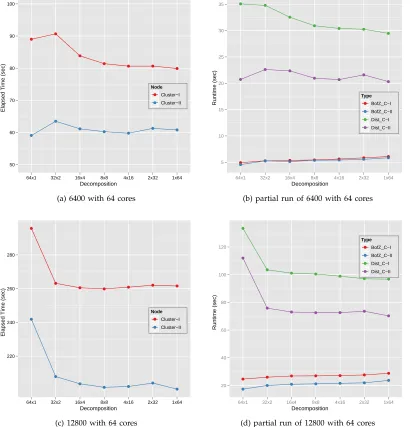
Also, Fig. 6-(a) and (c) show the overall elapsed time comparisons for the 6400 and 12800 PubChem data sets with respect to how to decompose the given

N×N matrices with 64 cores in I and

Cluster-II. Fig. 6-(b) and (d) illustrate the partial runtimes

related to the calculation ofB₍X_{) and the calculation}

of D₍X_{) of 6400 and 12800 PubChem data sets, the}

same as Fig. 5. Similar to Fig. 5, the data decompo-sition does not make a substantial difference in the overall runtime of the parallel SMACOF with a small data set. However, row-based decomposition, in this

case a64×1block decomposition, takes much longer

for running time than the other decompositions, when we run the parallel SMACOF with the 12800 points data set. If we compare Fig. 6-(c) with Fig. 6-(d), we can easily find that the overall performance with respect to data decomposition is mostly affected by the calculation of the distance matrix runtime for the 64 core experiment.

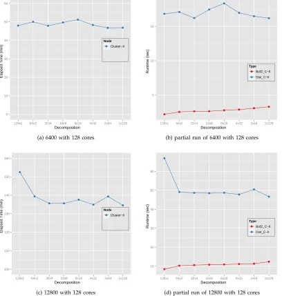
The performance of overall elapsed time and partial runtimes of the 6400 and 12800 Pubchem data sets

based on different decompositions of the givenN×N

matrices with 128 cores are experimented in only the Cluster-II system in Table 2. Those performance plots are shown in Fig. 7. As shown in Fig. 5 and Fig. 6, the data decomposition does not have a considerable impact on the performance of the parallel SMACOF with a small data set but it does have a significant influence on that performance with a larger data set. The main reason for the above data decomposition experimental results is the cache line effect that af-fects cache reusability, and generally balanced block decomposition shows better cache reusability so that it occurs with less cache misses than the skewed de-compositions [17], [18]. In the parallel implementation of the SMACOF algorithm, two main components actually access data multiple times so that will be

affected by cache reusability. One is the[N×N]·[N×D]

matrix multiplication part. Since we implement the matrix multiplication part based on the block matrix

multiplication method with a 64×64 block for the

purpose of better cache utilization, the runtime of matrix multiplication parts is almost the same without regard to data decomposition.

However, the distance matrix updating part is a tricky part. Since each entry of the distance matrix is accessed only once whenever the matrix is updated,

it is not easy to think about the entries reusability. Although each entry of the distance matrix is accessed only once per each update, the new mapping points are accessed multiple times for calculation of the distance matrix. In addition, we update the distance matrix row-based direction for better locality. Thus, it is better for the number of columns to be small enough so that the coordinate values of each accessed mapping points for updating the assigned distance sub-matrix remain in the cache memory as much as necessary.

Fig. 5-(b),(d) through Fig. 7-(b),(d) illustrate the cache reusability effect on 6400 points data and 12800 points data. For instance, for the row-based

decom-position case, p×1 decomposition, each process is

assigned anN/p×N block, i.e.100×6400data block

for the cases ofN= 6400andp= 64. WhenN = 6400,

the runtime of the distance matrix calculation part does not make much difference with respect to the data decomposition. We might consider that, if the number of columns of the assigned block is less than or equal to 6400, then cache utilization is no more harmful for the performance of the distance matrix calculation part of the parallel SMACOF. On the other

hand, when N = 12800 which is doubled, the

run-time of the distance matrix calculation part of

row-based decomposition (p×1), and which is assigned

a 12800/p× 12800 data block for each process, is

much worse than the other data decomposition cases, as in sub-figure (d) of Fig. 5 - Fig. 7. For the other

decomposition cases, such as p/2×2 through 1×p

data decomposition cases, the number of columns of the assigned block is less than or equal to 6400, when

N = 12800, and the runtime performance of distance

matrix calculation part of those cases are similar to each other and much less than the row-based data decomposition.

We have also investigated the runtime of theB₍X₎

calculation, since the message passing mechanism for

computing B₍X_{) is different based on data}

decom-position. Since the diagonal elements ofB₍X_{) are the}

negative sum of elements in the corresponding rows,

it is required to callMPI_AllreduceorMPI_Reduce

MPI APIs for each row-communicator. Thus, the less number of column blocks means faster (or less MPI

overhead) processes in computing B₍X_{), and even}

the row-based decomposition case does not need to

call the MPI API for calculatingB₍X_{). The effect of}

the different message passing mechanisms ofB₍X_{) in}

regard to data decomposition is shown in sub-figure (b) and (d) of Fig. 5 through Fig. 7.

Decomposition

Elapsed Time (sec)

50 60 70 80 90 100

64x1 32x2 16x4 8x8 4x16 2x32 1x64

Node

Cluster−I Cluster−II

(a) 6400 with 64 cores

Decomposition

Runtime (sec)

5 10 15 20 25 30 35

64x1 32x2 16x4 8x8 4x16 2x32 1x64

Type

BofZ_C−I BofZ_C−II Dist_C−I Dist_C−II

(b) partial run of 6400 with 64 cores

Decomposition

Elapsed Time (sec)

220 240 260 280

64x1 32x2 16x4 8x8 4x16 2x32 1x64

Node

Cluster−I Cluster−II

(c) 12800 with 64 cores

Decomposition

Runtime (sec)

20 40 60 80 100 120

64x1 32x2 16x4 8x8 4x16 2x32 1x64

Type

BofZ_C−I

BofZ_C−II Dist_C−I Dist_C−II

(d) partial run of 12800 with 64 cores

Fig. 6. Overall Runtime and partial runtime of parallel SMACOF for 6400 and 12800 PubChem data with 64

cores in Cluster-I and Cluster-II w.r.t. data decomposition ofN×N matrices.

and Networks. The L2 cache size per core is 3 times bigger in Cluster-II than in Cluster-I, and Cluster-II is connected by 20Gbps Infiniband but Cluster-I is connected via 1Gbps Ethernet. Since SMACOF with large data is a memory-bound application, it is natural that the bigger cache size results in the faster running time.

4.2 Performance Analysis of the Efficiency and

Scalability

In addition to data decomposition experiments, we measured the parallel scalability of parallel SMACOF

in terms of the number of processesp. We investigated

the scalability of parallel SMACOF by running with

different number of processes, e.g. p = 64, 128, 192,

and 256. On the basis of the above data decomposition

experimental results, the balanced decomposition has

been applied to this process scaling experiments. Asp

increases, the elapsed time should decrease, but linear performance improvement could not be achieved due to the parallel overhead.

We make use of the parallel efficiency value with respect to the number of parallel units for the purpose of measuriing scalability. Eq. (12) and Eq. (13) are the equations of overhead and efficiency calculations:

f = pT(p)−T(1)

T(1) (12)

ε= 1

1 +f =

T(1)

pT(p) (13)

Decomposition

Elapsed Time (min)

0 10 20 30 40 50 60

128x1 64x2 32x4 16x8 8x16 4x32 2x64 1x128

Node

Cluster−II

(a) 6400 with 128 cores

Decomposition

Runtime (sec)

5 10 15

128x1 64x2 32x4 16x8 8x16 4x32 2x64 1x128

Type

BofZ_C−II Dist_C−II

(b) partial run of 6400 with 128 cores

Decomposition

Elapsed Time (min)

100 110 120 130 140 150 160

128x1 64x2 32x4 16x8 8x16 4x32 2x64 1x128

Node

Cluster−II

(c) 12800 with 128 cores

Decomposition

Runtime (sec)

10 20 30 40 50 60

128x1 64x2 32x4 16x8 8x16 4x32 2x64 1x128

Type

BofZ_C−II Dist_C−II

(d) partial run of 12800 with 128 cores

Fig. 7. Overall Runtime and partial runtime of parallel SMACOF for 6400 and 12800 PubChem data with 128

cores in Cluster-II w.r.t. data decomposition ofN×N matrices.

running time with p parallel units, and T(1) is the

sequential running time. In practice, Eq. (12) and Eq. (13) can be replaced with Eq. (14) and Eq. (15) as follows:

f =αT(p1)−T(p2)

T(p2)

(14)

ε= 1

1 +f =

T(p2)

αT(p1) (15)

where α = p1/p2 and p2 is the smallest number of

used cores for the experiment, so α ≥ 1. We use

Eq. (14) and Eq. (15) in order to calculate the overhead and corresponding efficiency, since it is impossible to run in a single machine for 50k and 100k data sets. Note that we used 16 computing nodes in Cluster-II

(total memory size in 16 computing nodes is 768 GB) to perform the scaling experiment with a large data set, i.e. 50k and 100k PubChem data, since the SMA-COF algorithm requires 480 GB memory for dealing with 100k data points, as we disscussed in Section 3.1, and Cluster-II can only perform that with more than 10 nodes.

The elapsed time of the parallel SMACOF with two large data sets, 50k and 100k, is shown in Fig. 8-(a), and the corresponding relative efficiency of Fig. 8-(a) is shown in Fig. 8-(b). Note that both coordinates are log-scaled, in Fig. 8-(a). As shown in Fig. 8-(a), the par-allel SMACOF achieved performance improvement as

the number of parallel units (p) increases. However,

the performance enhancement ratio (a.k.a. efficiency)

number of processes

Elapsed Time (sec)

210

210.5

211

211.5

212

212.5

213

26 ₂6.5 ₂7 ₂7.5 ₂8 Size

100k

50k

(a) large data runtime

number of processes

Efficiency

0.0 0.2 0.4 0.6 0.8 1.0

100 150 200 250

Size

100k

50k

(b) large data efficiency

Fig. 8. Performance of parallel SMACOF for 50K and 100K PubChem data in Cluster-II w.r.t. the number of processes, i.e. 64, 128, 192, and 256 processes (cores). (a) shows runtime and efficiency is shown at (b). We

choose balanced decomposition as much as possible, i.e.8×8for 64 processes. Note that both x and y axes

are log-scaled for (a).

in Fig. 8-(b). A reason for reducing efficiency is that the ratio of the message passing overhead over the assigned computation per each process is increased due to more message overhead and less computing

portion per process aspincreases, as shown in Table 3.

Another reason for efficiency decrease is the memory bandwidth effect, since we used a fixed number of nodes (16 nodes) for the experiments with the large data sets, due to large memory requirement for large data sets, and have increased the used number of cores per node to increase the parallel units.

Table 3 is the result of the runtime analysis of the parallel matrix multiplication part of the proposed parallel SMACOF implementation which detached the time of the pure block matrix multiplication com-putation part and the time of the MPI message pass-ing overhead part for parallel matrix multiplication, from the overall runtime of the parallel matrix mul-tiplication part of the parallel SMACOF

implementa-tion. Note that#Procs, tMatMult,tMM Computing,

and tMM Overhead represent the number of pro-cesses (parallel units), the overall runtime of the par-allel matrix multiplication part, the time of the pure block matrix multiplication computation part, and the time of the MPI message passing overhead part for parallel matrix multiplication, respectively.

Theoretically, thetMM Computingportion should

be negatively linear with respect to the number of par-allel units, if the number of points is the same and the

load balance is achieved. Also, the tMM Overhead

portion should be increased as the number of parallel units is increased, if the number of points is the same.

More specifically, if MPI_Bcast is implemented as

one of the classical algorithms, such as a binomial tree or a binary tree algorithm [19], in MPI.NET library,

then the tMM Overhead portion will follow

some-whatO(⌈lgp⌉)with respect to the number of parallel

units (p), since theMPI_Bcastroutine in Alg. 3 could

be the most time consuming MPI method among the MPI routines of parallel matrix multiplication due in part to the large message size and the maximum number of communication participants.

Fig. 9 illustrates the efficiency (calculated by

Eq. (15)) of tMatMult and tMM Computing in

Ta-ble 3 with respect to the number of processes. As shown in Fig. 9, the pure block matrix multiplication part shows very high efficiency, which is almost ONE. In other words, the pure block matrix multiplication part of the parallel SMACOF implementation achieves linear speed-up as we expected. Based on the

effi-ciency measurement oftMM Computingin Fig. 9, we

could conclude that the proposed parallel SMACOF implementation achieved good enough load balance and the major component of the decrease of the efficiency is the compulsary MPI overhead for imple-menting parallelism. By contrast, the efficiency of the overall runtime of the parallel matrix multiplication part is decreased to around 0.5, as we expected based on Table 3.

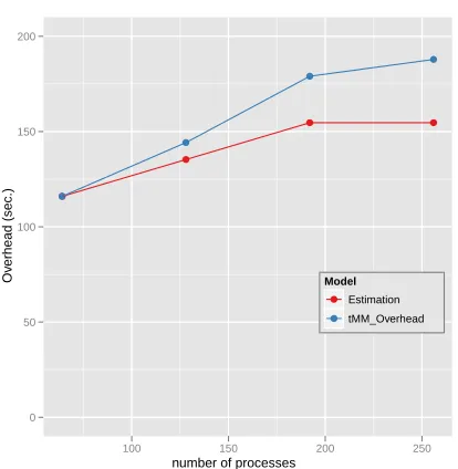
We also compare the measured MPI overhead of the

parallel matrix multiplication (tMM Overhead) in

Ta-ble 3 with the estimation of the MPI overhead with re-spect to the number of processes. The MPI overhead is

TABLE 3

Runtime Analysis of Parallel Matrix Multiplication part of parallel SMACOF with 50k data set in Cluster-II

#Procs tMatMult tMM Computing tMM Overhead

64 668.8939 552.5348 115.9847

128 420.828 276.1851 144.2233

192 366.1 186.815 179.0401

256 328.2386 140.1671 187.8749

number of processes

Efficiency

0.0 0.2 0.4 0.6 0.8 1.0

100 150 200 250

Portion

MM_Computing

tMatMult

Fig. 9. Efficiency oftMatMultandtMM Computing

in Table 3 with respect to the number of processes.

is implemented by a binomial tree or a binary tree

algorithm, so that the runtime of MPI_Bcast is in

O(⌈lg(p)⌉)with respect to the number of parallel units

(p). The result is described in Fig. 10. In Fig. 10, it

is shown that the measured MPI overhead of the parallel matrix multiplication part has a similar shape with estimation overhead. We could conclude that the measured MPI overhead of the parallel matrix multiplication part takes the expected amount of time. In addition to the experiment with pubChem data, which is represented by a vector format, we also experimented on the proposed algorithm with other real data sets, which contains 30,000 biological se-quence data with respect to the metagenomics study (hereafter MC30000 data set). Although it is hard to present a biological sequence in a feature vector, researchers can calculate a dissimilarity value between two different sequences by using some pairwise se-quence alignment algorithms, like Smith Waterman - Gotoh (SW-G) algorithm [20], [21] which we used here.

Fig. 11 shows: (a) the runtime; and (b) the effi-ciency of the parallel SMACOF for the MC30000 data in Cluster-I and Cluster-II in terms of the number of processes. We tested it with 32, 64, 96, and 128

number of processes

Ov

erhead (sec.)

0 50 100 150 200

100 150 200 250

Model

Estimation

tMM_Overhead

Fig. 10. MPI Overhead of parallel matrix multiplication (tMM Overhead) in Table 3 and the rough Estimation of the MPI overhead with respect to the number of processes.

processes for Cluster-I, and experimented on it with more processes, i.e. 160, 192, 224, and 256 processes, for Cluster-II. Both (a) and (b) sub-figure of Fig. 11 show similar tendencies to the corresponding sub-figure of Fig. 8. In contrast to the experiments of large pubchem data sets, we fixed the number of cores used per node (8 cores per node) in the experiments of MC30000 data set, and increased the number of nodes for the increase of paralle units. Therefore, we may assume that there is no memory bandwidth effect for the decrease of the efficiency related to Fig. 11.

5

R

W

number of processes

Elapsed Time (sec)

28.5

29

29.5

210

210.5

211

25 ₂5.5 ₂6 ₂6.5 ₂7 ₂7.5 ₂8 System

Cluster−I

Cluster−II

(a) MC30000 runtime

number of processes

Efficiency

0.0 0.2 0.4 0.6 0.8 1.0

50 100 150 200 250

System

Cluster−I

Cluster−II

(b) MC30000 efficiency

Fig. 11. Performance of parallel SMACOF for MC 30000 data in Cluster-I and Cluster-II w.r.t. the number of processes, i.e. 32, 64, 96, and 128 processes for Cluster-I and Cluster-II, and extended to 160, 192, 224, and 256 processes for Cluster-II. (a) shows runtime and efficiency is shown at (b). We choose balanced decomposition

as much as possible, i.e.8×8for 64 processes. Note that both x and y axes are log-scaled for (a).

multiple populations as proposed in [25], but not for dealing with larger data sets in MDS. Pawliczek et. al. [26] proposed a parallel implementation of MDS method for the purpose of visualizing large datasets of multidimensional data. Instead of using traditional approaches, which utilize minimization methods to find an optimal (or local optimal) mapping of the STRESS function, they proposed a heuristic method based on particle dynamics in [26]. In addition to the above parallel efforts on MDS methods, a threading-based shared memory parallel implementation of SMACOF algorithm was also proposed in [18].

6

C

F

W

In this paper, we have described a well-known di-mension reduction algorithm, called MDS (SMACOF), and we have discussed how to utilize the algorithm for a huge data set. The main issues involved in dealing with a large amount of data points are not only lots of computations but also huge memory requirements. Parallelization via the traditional MPI approach in order to utilize the distributed memory computing system, which can support much more computing power and extend the accessible memory size, is proposed as a solution for the amendment of the computation and memory shortage so as to be able to treat large data with SMACOF.

As we discussed in the performance analysis, the data decomposition structure is important to maxi-mize the performance of the parallelized algorithm since it affects message passing routines and the

message passing overhead as well as the cache-line effect. We look at overall elapsed time of the parallel SMACOF based on data decomposition as well as sub-routine runtimes, such as calculation of BofZ matrix (B₍X_{)) and distance matrix (}D₍X_{)). The cache}

reusability affects the performance of updating the distance matrix of the newly generated mappings with respect to the data decomposition if we run a large data set. From the above analysis, balanced data

decomposition (m×n) is generally better than skewed

decomposition (p×1 or 1×p) for the parallel MDS

algorithm.

In addition to data decomposition analysis, we also analyzed the efficiency and the scalability of the par-allel SMACOF. Although the efficiency of the parpar-allel SMACOF is decreased by increasing the number of processes due to the increase of overhead and the de-crease of pure parallel computing time, the efficiency is still good enough for a certain degree of parallelism.

Based on the fact that the tMM Computing in

Ta-ble 3 achieved almost linear speedup as in Fig. 9, it is shown that the parallel SMACOF implementation deals with the load balance issue very well and the inevitable message passing overhead for parallelism is the main factor of the reduction of the efficiency.

(called sample data), and the dimension reduction of the remaining points are interpolated based on the pre-mapped mapping position of the sample data. The detail of the interpolation approach is reported in [27].

In [1], [28], we investigated the overhead of pure MPI and hybrid (MPI-Threading) model with mul-ticore cluster systems. In [1], pure MPI outperforms hybrid model for the application with relatively fast message passing synchronization overhead. However, for the case of high MPI synchronization time, hy-brid model outperforms pure MPI model with high parallelism. Since the MPI overhead is grown as the number of processes is increased in Fig. 10, it is worth to investigate hybrid model SMACOF.

R

[1] G. Fox, S. Bae, J. Ekanayake, X. Qiu, and H. Yuan, “Parallel data mining from multicore to cloudy grids,” in Proceedings of HPC 2008 High Performance Computing and Grids workshop, Cetraro, Italy, July 2008.

[2] C. Bishop, M. Svens´en, and C. Williams, “GTM: A principled alternative to the self-organizing map,” Advances in neural information processing systems, pp. 354–360, 1997.

[3] ——, “GTM: The generative topographic mapping,” Neural computation, vol. 10, no. 1, pp. 215–234, 1998.

[4] T. Kohonen, “The self-organizing map,” Neurocomputing, vol. 21, no. 1-3, pp. 1–6, 1998.

[5] W. S. Torgerson, “Multidimensional scaling: I. theory and method,”Psychometrika, vol. 17, no. 4, pp. 401–419, 1952. [6] J. B. Kruskal and M. Wish,Multidimensional Scaling. Beverly

Hills, CA, U.S.A.: Sage Publications Inc., 1978.

[7] I. Borg and P. J. Groenen, Modern Multidimensional Scaling: Theory and Applications. New York, NY, U.S.A.: Springer, 2005. [8] J. Y. Choi, S.-H. Bae, X. Qiu, and G. Fox, “High per-formance dimension reduction and visualization for large high-dimensional data analysis,” in Proceedings of the 10th IEEE/ACM International Symposium on Cluster, Cloud and Grid Computing (CCGRID) 2010, May 2010, pp. 331–340.

[9] J. de Leeuw, “Applications of convex analysis to multidimen-sional scaling,”Recent Developments in Statistics, pp. 133–145, 1977.

[10] ——, “Convergence of the majorization method for multidi-mensional scaling,”Journal of Classification, vol. 5, no. 2, pp. 163–180, 1988.

[11] J. B. Kruskal, “Multidimensional scaling by optimizing good-ness of fit to a nonmetric hypothesis,”Psychometrika, vol. 29, no. 1, pp. 1–27, 1964.

[12] Y. Takane, F. W. Young, and J. de Leeuw, “Nonmetric individ-ual differences multidimensional scaling: an alternating least squares method with optimal scaling features,”Psychometrika, vol. 42, no. 1, pp. 7–67, 1977.

[13] T. Hofmann and J. M. Buhmann, “Pairwise data clustering by deterministic annealing,”IEEE Transactions on Pattern Analysis and Machine Intelligence, vol. 19, pp. 1–14, 1997.

[14] A. Dempster, N. Laird, and D. Rubin, “Maximum likelihood from incomplete data via the em algorithm,” Journal of the Royal Statistical Society. Series B, pp. 1–38, 1977.

[15] E. H. Moore, “On the reciprocal of the general algebraic matrix,”Bulletin of American Mathematical Society, vol. 26, pp. 394–395, 1920.

[16] R. Penrose, “A generalized inverse for matrices,”Proceedings of the Cambridge Philosophical Society, vol. 51, pp. 406–413, 1955. [17] X. Qiu, G. C. Fox, H. Yuan, S.-H. Bae, G. Chrysanthakopoulos, and H. F. Nielsen, “Data mining on multicore clusters,” in

Proceedings of 7th International Conference on Grid and Coopera-tive Computing GCC2008. Shenzhen, China: IEEE Computer Society, Oct. 2008, pp. 41–49.

[18] S.-H. Bae, “Parallel multidimensional scaling performance on multicore systems,” in Proceedings of the Advances in High-Performance E-Science Middleware and Applications workshop (AHEMA) of Fourth IEEE International Conference on eScience. Indianapolis, Indiana: IEEE Computer Society, Dec. 2008, pp. 695–702.

[19] J. Pjeˇsivac-Grbovi´c, T. Angskun, G. Bosilca, G. Fagg, E. Gabriel, and J. Dongarra, “Performance analysis of mpi collective operations,” Cluster Computing, vol. 10, no. 2, pp. 127–143, 2007.

[20] T. F. Smith and M. S. Waterman, “Identification of common molecular subsequences,”Journal of molecular biology, vol. 147, no. 1, pp. 195–197, 1981.

[21] O. Gotoh, “An improved algorithm for matching biological sequences,” Journal of Molecular Biology, vol. 162, no. 3, pp. 705–708, 1982.

[22] D. Goldberg, Genetic algorithms in search, optimization, and machine learning. Addison-wesley, 1989.

[23] R. Mathar and A. ˇZilinskas, “On global optimization in two-dimensional scaling,” Acta Applicandae Mathematicae, vol. 33, no. 1, pp. 109–118, 1993.

[24] A. Varoneckas, A. Zilinskas, and J. Zilinskas, “Multidimen-sional scaling using parallel genetic algorithm,” Computer Aided Methods in Optimal Design and Operations, pp. 129–138, 2006.

[25] E. Cantu-Paz,Efficient and accurate parallel genetic algorithms. Springer, 2000, vol. 1.

[26] P. Pawliczek and W. Dzwinel, “Parallel implementation of multidimensional scaling algorithm based on particle dynam-ics,” inParallel Processing and Applied Mathematics, ser. Lecture Notes in Computer Science, R. Wyrzykowski, J. Dongarra, K. Karczewski, and J. Wasniewski, Eds., vol. 6067. Springer Berlin / Heidelberg, 2010, pp. 312–321.

[27] S.-H. Bae, J. Y. Choi, X. Qiu, and G. Fox, “Dimension reduction and visualization of large high-dimensional data via interpo-lation,” inProceedings of the ACM International Symposium on High Performance Distributed Computing (HPDC) 2010, Chicago, Illinois, June 2010.