Shape Clustering and Spatial temporal Constraint for Non rigid Structure from Motion

(1)

Shape Clustering and Spatial-temporal

Constraint for Non-rigid Structure from

Motion

Huizhong Deng

B. Eng. (Honours)

Australian National University

September 2016

A thesis submitted for the degree of Master of Philosophy

at The Australian National University

Computer Vision Group

Research School of Engineering

(2)

Declaration

The contents of this thesis are the results of original research and have not been

submitted for a higher degree to any other university or institution.

Part of the work in this thesis has been published as conference proceedings.

Conferences

1. H. Deng and Y. Dai, ”Pushing the limit of non-rigid structure-from-motion by

shape clustering,” 2016 IEEE International Conference on Acoustics, Speech

and Signal Processing (ICASSP), Shanghai, 2016, pp. 1999-2003.

(3)

ii

The research work presented in this thesis has been performed jointly with Dr.

Yuchao Dai. The substantial majority of this work was my own.

Huizhong Deng

Research School of Engineering College of Engineering and Computer Science,

The Australian National University,

Canberra,

ACT,

(4)

Acknowledgements

The work presented in this thesis would not have been possible without the support

of a number of individuals and organizations and they are gratefully acknowledged

below.

First of all, I would like to give my sincere appreciation to my supervisor,

Dr. Yuchao Dai. He guided me through my two-year research, gave me useful

suggestions towards various problems and shared me his knowledge. I have learned

both professional skills and research methods from him.

Secondly, thanks to my fellow research student, Jiayan Qiu, who acted like my mentor and shared me his research experiences.

I am also grateful to the administrative staff in the college who helped me with

problems regarding the program.

Finally, I am thankful to my girlfriend and family, who gave me both moral

and financial support to finish the research.

(5)

Abstract

Non-rigid Structure-from-Motion (NRSfM) is an active research field in computer

vision. The task of NRSfM is to simultaneously recover camera motion and 3D

structure from 2D tracks of a deformable object. This problem is generally

catego-rized into sparse and dense cases in terms of scale, where sparse NRSfM deals with

a few feature tracks and dense NRSfM recovers the 3D position of each pixel in

an image flow. As NRSfM is essentially an under-constrained problem, recent

re-search has focused on enforcing priors to reliably solve the problem. In this thesis,

we propose a shape clustering method for sparse NRSfM and a spatial-temporal constraint for dense NRSfM.

For sparse NRSfM, we first revisit the concept of “reconstructability”, which

indicates the possibility of reconstructing a 3D shape, given 2D feature tracks and

camera motion. We give an extension to it and define “reconstructability” from

3D shape complexity and motion complexity. To increase global reconstructability,

we then propose an iterative shape clustering method to divide a sequence into

several sub-sequences, thus decreasing the shape complexity of each sub-sequence,

which is much easier to solve individually. Our method aims at solving the

long-term, complex motions, which have been a difficult task for previous methods. Experimental results show that our method outperforms the current

state-of-the-art methods by a margin, thus pushing the limit of sparse NRSfM.

For dense NRSfM, we first revisit the temporal smoothness utilized in sparse

NRSfM and demonstrate that it can be employed for dense case directly. Secondly,

we propose a spatial smoothness constraint by enforcing a Laplacian filter to the

shape matrix. Finally, to handle real world noise and outliers in measurements,

we robustify the data term by using the L1 norm. Our method gives a simple

yet elegant convex least-squares optimization, which can be effectively solved by

gradient descent. Experimental results on both synthetic and real images show that the proposed method achieves state-of-the-art performance in dense NRSfM.

(6)

List of Acronyms

NRSfM Non-rigid Structure-from-Motion

2D Two-Dimensional

3D Three-Dimensional

SfM Structure-from-Motion

SVD Singular Value Decomposition

EM Expectation-Maximization

PND Procrustean Normal Distribution

PPCA Probabilistic Principle Component Analysis

SDP Semidefinite programming

DCT Discrete Cosine Transform

MND Matrix Normal Distribution

CMU Carnegie Mellon University

UMPM Utrecht Multi-Person Motion

PCA Principle Component Analysis

RMS Root Mean Squared

(7)

List of Figures

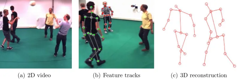
1.1 Illustration of NRSfM procedure. (a) 2D video. (b) 2D video with

tracked feature points. (c) 3D reconstruction result. Figures (a) and

(b) are taken from [1]. . . 2

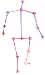
1.2 Illustration of Sparse NRSfM. The result is obtained using our shape

clustering method. Red circles are 3D ground truth points, and blue

crosses are reconstructed 3D points. . . 3

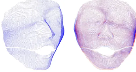
1.3 Illustration of dense NRSfM. The result is obtained using our spatial-temporal method. Red dots are 3D ground truth points, and blue

dots are reconstructed 3D points. . . 4

3.1 Illustration of our method on the UMPM “Free” sequence. The top row

shows the result by PND [2] using a global model while the bottom row

shows the result by our method, where the whole sequence is clustered

into 3 subsequences. The dimensionality of the subspace (rank) is shown

alongside the corresponding results. Different colors are used to indicate

the clustering result of the frames. Through iterative shape clustering

and 3D shape reconstruction, we achieved an overall 3D error as 0.2588

while the state-of-the-art method PND achieved 0.3887. . . 22 3.2 Numerical experiments analyzing the relationship between shape

com-plexity, motion complexity and 3D reconstruction performance. (a) 3D

reconstruction error on the “Triangle” sequence with varying shape

com-plexity under different camera rotation speeds. (b) 3D reconstruction

error for different UMPM sequences with varying shape complexity

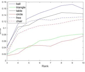
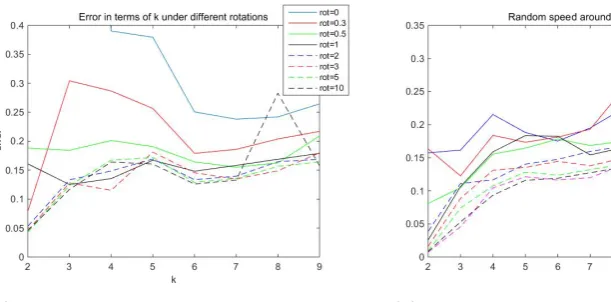
un-der completely random camera motions. . . 25 3.3 Experiments with more realistic camera motions. (a) 3D reconstruction

error on the “Table” sequence with varying shape complexity under

con-stant camera rotation speeds. (b) 3D reconstruction error on the “Table” sequence with varying shape complexity under random camera rotation

speeds. . . 26

(10)

List of Figures ix

3.4 3D reconstruction results on different sequences under different

configu-rations. . . 29 3.5 3D reconstruction results of our method (top row) and PND (bottom

row) on UMPM dataset. “◦” indicates ground truth and “+” indicates 3D reconstruction points. Parameters: K = 3, σ = 10. Sequences from

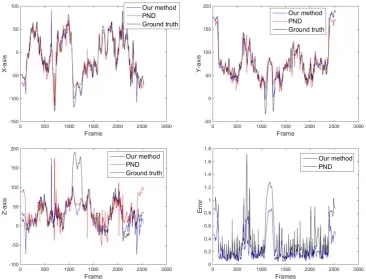
left to right: circle, free, table, triangle. . . 30 3.6 Top left, top right, bottom left: a point trajectory in ”Free” sequence

showing X,Y,Z coordinates, respectively. Bottom right: error of each

frame in ”Free” sequence. . . 32

4.1 Evolution from 2D to robust 3D shape on Synthetic Face Sequence 2 [3]

in the presence of outliers. From left to right: input W; Pseudo-inverse

results; Temporal smooth results; Spatial-temporal smooth results;

Ro-bust spatial-temporal smooth results. Top row: 4th frame; Bottom row:

6th frame. e denotes the RMS 3D error of the full 3D reconstruction

under each scenario. . . 34 4.2 Temporal smoothness experiment on a dense sequence, with different

trade-off parameter λ. (a) 3D reconstruction error; (b) Temporal

smoothness cost; (c) Reprojection error. . . 37

4.3 Evolution of dense 3D shape with different trade-off parameters. Top

row: pseudo-inverse result (λ = 0); Middle row: temporal smooth

result (λ= 10−3_{); Bottom row: rigid result (}_λ_{= 10}5_{). . . .} ₃₈

4.4 Side view of the 3 results from left to right, where the trade-off

parameter λ gradually increase from 0 to ∞. . . 38 4.5 Our Laplacian filter (far right): 8-direction, sum of the 4 basic

Lapla-cian filters. . . 39

4.6 Left: temporal smooth result. Right: spatial-constrained result with

λ1 = 0, λ2 = 1 using temporal smoothness initialization. Top row:

front view, Bottom row: side view. . . 39

4.7 Experimental results on noisy data. Left: temporal constraint only;

Right: spatial-temporal constraint. Top: front view. Bottom: side

view. . . 40

4.8 Experimental results on data with outliers. Left: L2-norm on all

terms; Right: L1-norm on data term, L2-norm on the rest. Top:

(11)

List of Figures x

4.9 Results of synthetic face sequences using spatial-temporal constraints.

Red: ground truth; Blue: 3D reconstruction result. Parameters used:

λ1 = 10−3, λ2 = 1. Top row: front view. Bottom row: side view. The

last frame is used to present the results. . . 45 4.10 Top row: real 2D videos from left to right: Face, Back and Heart,

re-spectively. Middle and bottom row: results of dense sequences obtained

by spatial-temporal smoothness. Sub-figure (a) to (c) are the front views

of the respective sequences, and (d) to (f) are the side views. The last

frame is used to present the results. . . 46 4.11 (a) Curves of 3D error on synthetic sequences with noise. Noise

ratios are selected at 0%, 1%, 2%, 3%, 4%, and 5%. (b) Curves

of 3D error on synthetic sequences with outliers. Outlier ratios are

selected at 0%, 2%, 4%, 6%, 8%, and 10%. . . 46

4.12 Results of noisy W with σn = 0.02 max{W} with different parameters.

Sub-figure (a) to (d) are the front views of the face sequence, and (e) to

(12)

List of Tables

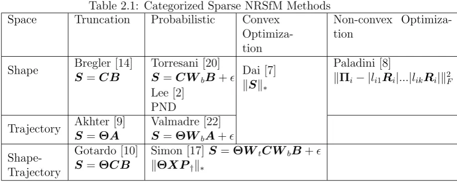
2.1 Categorized Sparse NRSfM Methods . . . 17

4.1 Quantitative evaluation on 4 synthetic face sequences. (Average RMS 3D

reconstruction error.) . . . 44

(13)

Chapter 1 Introduction

Non-rigid Structure-from-Motion (NRSfM) is an active research area in computer

vision. Given a series of 2D tracks taken by a monocular camera, NRSfM

si-multaneously solves the camera motion and 3D reconstruction of a deformable

object. Currently, state-of-the-art NRSfM techniques can handle moderate non-rigid deformation (i.e. facial expression and human body motion, etc.) from sparse

feature correspondences [4] [5] [6] [2] [7] [8] [9] [10] or dense pixel-level

trajecto-ries [11] [3] [12] [13]. This thesis aims at further improving the performance of

NRSfM in both sparse and dense scenarios, using different techniques for each.

In this chapter, we briefly introduce the concept of NRSfM, then give a summary

of sparse and dense NRSfM cases, respectively, and finally state our contributions.

1.1 Non-rigid Structure-from-Motion

Despite the recent progress stated above, NRSfM still lags far behind its rigid

counterpart, which is well-developed and can be reliably solved. This is mainly

due to the difficulty in modeling real world non-rigid variation [14] [15] [16] [17]

and the difficulty in the corresponding minimization problem [18]. Overall, NRSfM

is an under-determined problem, where 3D shapes are to be reconstructed from

monocular 2D images, and there are more variables than measurements. Therefore,

additional constraints must be added to make the problem solvable. Without using

priors, it is quite challenging to find an appropriate constraint to solve NRSfM. Figure 1.1 shows an illustration of NRSfM procedure. We start from a raw 2D

video of a deforming object, get the 2D tracks using certain tracking methods, and

solve the camera motion and 3D structure simultaneously.

(14)

1.2 Sparse NRSfM 2

[image:14.595.126.522.93.225.2]

(a) 2D video (b) Feature tracks (c) 3D reconstruction

Figure 1.1: Illustration of NRSfM procedure. (a) 2D video. (b) 2D video with tracked feature points. (c) 3D reconstruction result. Figures (a) and (b) are taken from [1].

1.2 Sparse NRSfM

The rigid Structure-from-Motion problem is reliably solved using factorization [19].

However, the extension to NRSfM, even in sparse case, was never implemented until

the 21th century. Figure 1.2 shows a simple demonstration of sparse NRSfM. The sequence contains 15 feature points, forming a sparse human body connected by

virtual skeletons. In 2000, Bregler et al. extended the rigid factorization method to the non-rigid scenario in their seminal work [14], where they considered the 3D

shapes being a linear combination of a series of shape bases. The shape space

method is then used along with other constraints, such as hierarchical priors [20],

metric projections [8] and rank minimization [7]. Meanwhile, Akhter et al. pro-posed a dual method to the shape space method, considering the 3D trajectory

of each point to be a linear combination of a pre-defined trajectory basis [9]. The

trajectory space method is then looked into by various authors, providing more the-oretical basis for the method [21] [22]. The shape and trajectory methods have also

been combined by Gotardo et al. , forming the shape space parameters into a tra-jectory space [10]. A probabilistic model is also proposed to constrain the shapes [2].

While most methods use the orthographic camera model, some researchers have

looked into solving the problem with a perspective model [23] [24] [25] [26] [21].

The above methods, however, are limited to simple motions, such as sit, stand

and walk, while a complex non-rigid variation is hard to be correctly represented

by a single subspace model or probabilistic model. Zhu et al. [27] represented complex deformations as lying in a union of subspaces rather than sum of subspaces. However, the solution involves a complex non-convex optimization.

In this thesis, we address the problem of long-term, complex motions by

(15)

1.3 Dense NRSfM 3

state-of-the-art method, spectral clustering is used to segment the whole sequence

into several shorter sub-sequences that individually contains a group of similar

shapes. Each subsequence is then individually solved to provide a better result,

which is fed into the next iteration of the process above. In a nutshell, our method

is an add-on based on a state-of-the-art method that is immune to sequence

per-mutation, and can decompose a complex problem into a few simple ones. We also

look into the concept of reconstructability that describes the possibility of

[image:15.595.289.363.268.392.2]

recon-structing a 3D shape, initially proposed by Park et al. [21], and generalize their idea to a wider span.

Figure 1.2: Illustration of Sparse NRSfM. The result is obtained using our shape clustering method. Red circles are 3D ground truth points, and blue crosses are reconstructed 3D points.

1.3 Dense NRSfM

Dense NRSfM is a much more complex problem than the sparse one, as a dense

surface can contain a huge number of points that is equal to the number of pixels in

an image. Figure 1.3 shows a simple demonstration of dense NRSfM. The sequence

contains 28,807 points, forming a dense surface of a human face. The density of

a point cloud introduces much more variables and computational complexity into

the problem. Therefore, most of the above sparse NRSfM methods are unable to

scale to the dense scenario. However, the continuity of a dense surface opens up

the possibility of applying a spatial constraint. In 2013, Garg et al. proposed the first dense NRSfM method using nuclear norm minimization and total variation [3].

However, their method requires a complex convex optimization and GPU is needed to speed up the implementation. Other methods utilize a segment-based procedure.

In the paper by Russel et al. [12], segmentation is performed on both object-level and part-object-level, then piece-wise reconstruction is applied by assuming locally

(16)

1.4 Main Contributions 4

track completion to deal with occlusions, then nuclear norm minimization is used

to recover the 3D shape. These methods directly process 2D images, but are

both computationally complex. Yu et al. [28] proposed to utilize the temporal smoothness in both camera motion and 3D deformation, which however required

a rigid shape template as an additional input.

To address the problems of the methods mentioned above, we propose a simple

dense NRSfM method based on spatial-temporal smoothness. The optimization

process is convex and simple, but has a very large size due to the huge number of variables in dense NRSfM. We solve this problem in an iterative manner using

gradient descent, thus eliminating the requirement of additional hardware. Our

[image:16.595.204.439.304.429.2]

method is fast, easy to implement, template-free and robust to noise and outliers.

Figure 1.3: Illustration of dense NRSfM. The result is obtained using our spatial-temporal method. Red dots are 3D ground truth points, and blue dots are recon-structed 3D points.

1.4 Main Contributions

The main contributions of this thesis are as follows:

1. We propose an improvement to existing sparse NRSfM methods that

de-composes a long-term complex problem into several short, simple ones, which are

easier to solve individually. We also propose a new definition of reconstructability

derived by the complexity of rotation and shape, explaining the possibility of 3D

reconstruction from a new angle. Our method further improves the performance

of state-of-the-art methods.

2. We propose a new template-free dense NRSfM method based on spatial-temporal constraints. We use the first-order difference matrix and a Laplacian filter

to enforce temporal smoothness and local spatial smoothness on the shapes. Our

(17)

1.5 Outline 5

hardware. It is also robust to severe noise and outliers. The performance of our

method is comparable to state-of-the-art methods.

1.5 Outline

The following content of this thesis is presented as follows: Chapter 2 introduces

the formulation and related research of both sparse NRSfM and dense NRSfM. Chapter 3 presents our approach of clustering-based NRSfM, provides the

experi-mental results on long-term complex sparse sequences, and explains our discovery

on reconstructability. Chapter 4 presentss our new dense NRSfM method using

spatial-temporal constraints, explains the evolution of 3D reconstruction under

different constraints, and shows plenty of experimental results under different

sce-narios. Chapter 5 gives a brief summary of the thesis and states some possible

(18)

Chapter 2 Background of

Non-Rigid-Structure-from-Motion

Recovering a 3D scene from a monocular video is a challenging task. Usually,

recovering a 3D scene from 2D at a specific time requires a stereo camera system

to provide multiple views of the scene from different camera poses. However, in

reality, most videos are taken by monocular cameras, such as digital cameras,

mobile phone cameras and security cameras. This makes Structure-from-Motion

become an active research area, where a 3D scene is recovered from a 2D video from

a monocular camera. Although SfM for a rigid scene is reliably solved, recovering

a non-rigid object is still a quite challenging task, as a time-varying object has

a unique structure at different time stamps. In this chapter, the development of NRSfM will be reviewed by showing various methods addressing the problem.

2.1 Formulation

2.1.1 Structure-from-Motion

Structure-from-Motion for a rigid scene is reliably solved using factorization by

Tomasi and Kanade [19]. Given a full set of 2D feature tracks obtained from a

monocular camera, SfM aims at simultaneously recovering the 3D structure and

camera poses. For a 2D feature sequence W1,W2,· · · ,WF with F frames, the

2D locations of each feature in a certain frame is expressed as:

Wi =

"

u1· · ·uP

v1· · ·vP

#

, (2.1)

(19)

2.1 Formulation 7

where each Wi containsP features. Assuming an orthographic camera model and

that the camera is centralized at the center of the object, we have:

Wi =RiS, (2.2)

where Ri ∈ R2×3 represents the first two rows of the rotation matrix of the i-th frame, and S ∈_R3×P _{contains the 3D positions of every point in the rigid shape.}

Stacking these matrices for all F frames gives:

W =RS, (2.3)

where W ∈_R2F×3P _and _R_∈

R2F×3 are the full measurement matrix and motion matrix, respectively.

Given W, we can apply the Singular Value Decomposition (SVD) such that

W =UΣVT. As R and S cannot be uniquely expressed using U, Σand V, we arrive at the following relationship:

W =UΣVT =U QQ−1ΣVT, (2.4) where ˆR = U Q, and ˆS = Q−1ΣVT. Under orthographic camera model, the 2×3 rotation matrix at the j-th frame Rj must be orthonormal, which is a key

constraint to solve the 3×3 matrix Q:

U2jQQTU2j = 1

U2jQQTU2j+1 = 0

U2j+1QQTU2j+1 = 1

, (2.5)

whereUk is the 1×3 rows ofU. The above equations provide plenty of constraints

for Q to be solved. Therefore, R and S have a closed-form solution.

2.1.2 Basics of Non-Rigid-Structure-from-Motion

In the non-rigid case, the 3D shapeS is no longer the same in every frame. Instead,

S represents a time-varying shape that has a unique structure for every frame.

Therefore, the measurement matrix of each frame Wi is calculated from a unique

(20)

2.1 Formulation 8 W =     R1 . .. RF     ·       S1 S2 .. . SF      

=RS, (2.6)

where R = blkdiag(R1,· · · ,RF) ∈ R2F×3F expresses the camera motion matrix, and S ∈_R3F×P

contains the non-rigid 3D shapes of each frame.

It is obvious that orthonormality constraint is not sufficient to directly solve

this problem, so additional constraints must be added. Bregleret al.[14] proposed a shape basis method, with the assumption that each non-rigid 3D shape is a linear

combination of a set of shape bases B1,B2, ...,BK:

S =

K

X

i=1

li·Bi S,Bi ∈R3×P. (2.7)

Based on this linear combination, the equation of NRSfM in a shape space becomes:

W =



 

l11R1 · · · lK1R1

l12R2 · · · lK2R2

l1FRF · · · lKFRF

  ·       B1 B2 . . . BK      

=R(C⊗I3)B=ΠB, (2.8)

whereC is the matrix that contains all shape basis coefficients. From the equation

above, it is clear that matrix W is of rank 3K. Therefore, the W matrix can be

decomposed via SVD to keep only the first 3K singular values:

W2F×P =U ·Σ·VT = ˆΠ2F×3K·Bˆ3K×P. (2.9)

Due to its non-uniqueness, the SVD of W is up to a 3K×3K correction matrix G:

W = ˆΠGG−1Bˆ =ΠB. (2.10)

By enforcing orthonormality constraint on ˆΠG, according to Xiao et al. [29], for each two-row of matrix Π, the following equation holds:

ˆ

Π2i−1:2iGGTΠˆ T

2i−1:2i = K

X

k=1

c2_ikI2×2, i= 1. . . F, k = 1. . . K, (2.11)

where Π2i−1:2i represents the i −th two-row of Π, and I2×2 is a 2×2 identity

(21)

2.2 Sparse NRSfM 9

equation above yields two linear constraints of GGT for each two-row of Π:

ˆ

Π2i−1GkGTkΠˆ T

2i−1 = ˆΠ2iGkGTkΠˆ T

2i

ˆ

Π2i−1GkGTkΠˆ T

2i = 0

, (2.12)

where Gk denotes the k-th column-triplet ofG.

Therefore, forF frames, there are 2F linear constraints. AsGGT is a 3K×3K

symmetric matrix, the number of unknowns is (9K2+3K)/2. Xiaoet al. stated that as long as the number of constraints is larger than unknowns, the solution can be

found via least-squares method. However, they also pointed out that the solutions

of the equations above are ambiguous, i.e. the shape bases and coefficients are not

unique. To form an unambiguous and closed-form solution, Xiao et al. proposed a basis constraint that the shapes in certain frames form the shape basis [29].

However, this method largely restricts the generality of NRSfM, because the

pre-defined shape basis does not necessarily represent all shapes in an image stream.

Later, Akhter et al. discovered that even the shape bases and coefficients are ambiguous, the shape itself is unique, only up to a global rotation [18]. In their paper, it is shown that an ambiguous solution ˆG can be transformed to the real

correction matrix G by multiplying each of its column triplets with a rotation

matrixV0. Therefore, the ambiguous shape solved from orthonormality constraints

is just a result of the real shape multiplied by a rotation matrixV0 on every frame,

which is a global rotation. Furthermore, they also stated that the real problem of

NRSfM lies in the optimization process, which is the reason why an increasing

number of methods are raised addressing more challenging tasks of NRSfM.

2.2 Sparse NRSfM

2.2.1 NRSfM in Shape Space

Ever since Bregler et al. ’s first shape basis method, many researchers have pro-posed various ways to optimize it, using different prior assumptions. Torresani et al. discovered a probabilistic model describing the shape coefficients. In their pa-per, a Probabilistic Principal Components Analysis (PPCA) shape model is used,

assuming that the shape coefficients have a Gaussian distribution. As a linear

transform of a Gaussian is still Gaussian, the 3D coordinates are also Gaussian.

(22)

2.2 Sparse NRSfM 10

model is described as follows:

zt∼ N(0 : I), (2.13)

st= ¯s+V zt+mt, (2.14)

p_t=Gt(st+Dt) +nt, (2.15)

where zt is the coefficients of shape basis having a Gaussian distribution,st is the

3D points vector at frame t, ¯s is the mean shape, V is the shape basis, p_t is the 2D points vector, Gt is the rotation matrix, Dt is the translation, and mt, nt are

zero-mean Gaussian vectors describing noise, with standard deviation ofσm andσn.

By combining the equations above, the distribution over p_t is given as:

p_t∼ N(Gt(¯s+Dt);Gt(V VT +σm2I)G T t +σ

2

nI)

The authors use an Expectation-Maximization (EM) algorithm to estimate the

parameters. The algorithm requires an initial guess of the basis coefficients, which

can be done with traditional methods, such as [29]. Then in the E-step, the

pos-terior distribution over zt is computed for each frame t. The following M-step

maximizes the joint likelihood of the measurementsp_1:_T, by updating each individ-ual parameters in a closed form. During the updating process, any missing data

will be filled in.

The authors also proposed a Linear Dynamics Model, where the shape

coef-ficients in each frame zt are related to the previous one, by multiplying a 3×3

translation matrix Θ. With this model assuming temporal smoothness over the

3D shapes, the method is improved when dealing with noise and missing data.

Paladiniet al. proposed a Metric Projection method to better solve the factor-ization problem [8]. Instead of optimizing the shape basisB, they directly optimize

the motion matrix Π and then update B and Π in an iterative manner. Recall

that the shape space factorization:

W =



 

l11R1 · · · lK1R1

l12R2 · · · lK2R2

l1FRF · · · lKFRF

  ·       B1 B2 . . . BK      

(23)

2.2 Sparse NRSfM 11

where the motion matrix at frame ihas the following structure:

Πi = [l1iRi· · ·lKiRi]. (2.17)

Therefore, the motion matrices have a distinct repetitive structure in the de-formable motion manifold [8]. The projection of a motion matrix to the manifold

yields the following least-squares problem:

min

Ri,li1,...,lik

kΠi− |li1Ri| −...− |likRi|k2F. (2.18)

The problem is unconstrained except thatRiis a 2×3 Stiefel matrix that follows the

orthonormality constraint. It can be decoupled by solving li1, ..., lik assuming fixed

Ri, and then solvingRi assuming fixed l. After the metric projection step,B(t) is

estimated by B(t) =Π(t)†W, andΠ(t+ 1) is estimated by Π(t+1) =W B(t)†. The optimization carries on until convergence. The method can also deal with missing

data, as the metric projection step also projects W onto the motion manifold. Later, Dai et al. proposed a prior-free method without any prior assumptions other than the orthonormality and low-rank constraint [7]. They improved the

process of estimating rotation matrix from orthonormality constraint using

trace-norm minimization, and also used trace-trace-norm minimization in shape optimization

resulting a convex problem. From the orthonormality constraint in Equation 2.12,

the problem narrows down to solving the matrixQ_k=GkGTk. Daiet al. discovered

a null-space representation of the vectorized version of matrixQ_k, from the formula

vec(AXBT) = (B⊗A)vec(X):

"

( ˆΠi⊗Πˆi)(1,:)−( ˆΠi⊗Πˆi)(4,:)

( ˆΠi⊗Πˆi)(2,:)

#

q_k =Aiqk= 0, (2.19)

where q_k = vec(Q_k). Stacking all such equations from all frames results in: Avec(Q_k) = Aq_k = 0. Therefore, the solution space of Q_k is the null space of A. It is also discovered that as Q_k =GkGTk, Qk must be rank-3 and positive

semi-definite. The final solution under noise-free condition becomes:

{Avec(Q_k) = 0} ∩ {Q_k0} ∩ {rank(Q_k) = 3}. (2.20)

Because the rank of Q_k is sensitive to noise, the rank 3 constraint is relaxed to a rank-minimization problem, and further relaxed to a trace-minimization problem

(24)

2.2 Sparse NRSfM 12

SDP solvers. Once Gk is obtained, the rotation matrix Ri for each frame can be

solved directly.

In terms of solvingS, in the expression of S = (C⊗I3)B, it is suggested that

rank(S)≤3K. However, Dai et al. found that the re-ordered expression of shape matrix S has a rank-K constraint:

S] =



  

X11 . . . X1P Y11 . . . Y1P Z11 . . . Z1P

..

. ... ... ... ... ...

XF1 . . . XF P YF1 . . . YF P ZF1 . . . ZF P



  

. (2.21)

The rank constraint is rank(S]) ≤ K, which is stronger than the rank-3K con-straint. This is relaxed to a rank-minimization problem, and further relaxed into

nuclear-norm minimization. Finally, the authors arrive at the following

optimiza-tion:

minµkS]k∗+

1

2kW −RSk

2

F. (2.22)

This is an SDP problem with a very large size (F ×3P). To avoid the inefficiency of solving such a large SDP, a numerical implementation based on fixed point

continuation was proposed. The gradient of 1₂kW −RSk2

F with respect to S ]

is calculated and then used for an iterative upgrading process to shrink S]. The solved S] is finally projected to the nearest rank-K matrix and rearranged to S.

Looking for a new way regarding NRSfM, Lee et al. [2] proposed a novel al-gorithm based on Procrustean alignment and a probabilistic model, called

Pro-crustean Normal Distribution (PND). In this method, the rank constraint used by

previous methods is eliminated, instead it is assumed that the 3D shapes follow

a Normal distribution after being Procrustean aligned. PND regards NRSfM as

a shape alignment problem, so that the rigid and non-rigid motions are strictly

separated. Moreover, the rotation matrix can be updated within the algorithm, which means rotation is not pre-processed in advance.

2.2.2 NRSfM in Trajectory Space

The shape space NRSfM has its inherent problem that basis is highly dependent on

the shape of the object. Akhter et al.[9] found a different view of NRSfM. Instead of expressing the shape in each frame as a linear combination of basis shapes,

they address each point trajectory across all frames as a linear combination of

basis trajectories. This method is object independent, because it focuses on the

motion of each single point, and assumes that the deformation must be temporal

(25)

2.2 Sparse NRSfM 13

Transform (DCT) basis is valid for reconstruction, thus reduces the number of

unknowns significantly.

The duality of shape space and trajectory space is shown in the rearranged form

of matrix S:

S] =



  

X11 . . . X1P Y11 . . . Y1P Z11 . . . Z1P

..

. ... ... ... ... ...

XF1 . . . XF P YF1 . . . YF P ZF1 . . . ZF P



   ,

where the row space of the matrix corresponds to shape space, and the column

space corresponds to trajectory space.

The time-varying structure is considered as a set of trajectories,T(i) = [Tx(i),Ty(i),Tz(i)],

whereT(i) includes the trajectories of thei-th point in a 3-dimension space. With

K trajectory bases, each trajectory is represented as a linear combination of basis

trajectory:

Tx(i) = k

X

j=1

axj(i)Θj (2.23)

where Θj is a trajectory basis vector, and axj(i) is the coefficient corresponding to

that basis vector. The same representation is used in y, z coordinates. The matrix S can be factorized into S3F×P =Θ3F×3kA3k×P, where A= [ATx, ATy, ATz]T and

Ax =



  

ax1(1) . . . ax1(P)

..

. ...

axk(1) . . . axk(P)



  

,Θ=

             

θT₁ θT 1 θT 1 .. . θT F θT F

θT_F               .

Same as before, the trajectory space NRSfM can be solved via factorization

with orthonormality constraints. The 2D coordinate matrix bW is factorized as

(26)

2.2 Sparse NRSfM 14

Q, we get

ˆ Λq1 =



  

θ1,1R1

.. .

θF,1RF



  

Using the orthonormality constraints, matrix q1 can be computed, and the

ro-tation matrices R can be estimated with a nonlinear minimization routine. Λ is

then computed by multiplying R and the pre-defined trajectory basis Θ. Finally,

the basis coefficients can be directly solved using the known W and Θ.

Park et al. [21] looked into the theoretical basis of 3D trajectories. They pro-posed a criterion called reconstructibility, which describes the possibility and

ac-curacy of reconstructing a 3D point from its 2D trajectory. Furthermore, they use a perspective camera model and solve it with Direct Linear Transform algorithm,

instead of the traditional factorization under orthographic model.

Specifically, the reconstructability η, characterizing the relationship between

camera motion, point motion and the trajectory basis, is defined as:

η(Θ) = kΘ

⊥_β⊥

Ck

kΘ⊥_β⊥

Xk

' How poorly Θ describesC

How poorly Θ describes X, (2.24)

where Θ is the pre-defined trajectory bases, C is the camera trajectory, while X

is the 3D point trajectory. In other words, a complex C and a simple X result in

a high value of η. The reconstructability can be enhanced by carefully choosing a DCT basis that describes the point trajectories well but not the camera trajectory.

Based on Parket al. ’s findings, Valmadre et al. [22] proposed a general trajec-tory prior for non-rigid reconstruction. The motivation lies in that the previously

defined reconstructibility is found to be flawed, as the theory does not consider

the choice of DCT basis size K, which may affect system condition significantly.

Additionally, the use of camera trajectory is not intuitive and prohibits the use of

affine cameras, which do not have camera centers. To address these problems, the

authors proposed a theoretical upper bound of 3D reconstruction error that

de-pends on the DCT basis size K, and a filter-based algorithm to automatically find

K by minimizing the basis’ response to a high-pass filter. The experiments show that this method can practically improve the over-smoothing problem of trajectory

(27)

2.2 Sparse NRSfM 15

2.2.3 NRSfM with Shape-Trajectory

The previous methods map a 3D shape into a linear subspace: shape space or

trajectory space. Gortardo et al. [10] proposed a combination of these models, called shape trajectory model, which describes the trajectory of a single point in a

K-dimensional shape space. This model assumes that the real objects deform in a

smooth way, making the model theoretically applicable.

As in shape basis, the 2D coordinate matrix W is factorized as W =R(C ⊗ I3)B = ΠB. Then the shape space coefficients C ∈ RF×K are described as

the trajectory of a single point in a K-dimensional shape space, with each row of

C being a point at one time instant. The column space of C, representing the

trajectory of each dimension, is described as a linear combination of d DCT basis

vectors:

C =Ωd[x1. . . xK] = ΩdX, X ∈Rd×K, (2.25) where Ωd is the DCT basis matrix with d bases, and X contains the coefficients

for the shape trajectory in DCT domain. Therefore, the factorized model of W is:

W =R(ΩdX ⊗I3)B=ΠB. (2.26)

As W is constrained to rank-3K by the linear combination of X, any number of

d=K, . . . , F can be considered, allowing better representation of higher-frequency

3D deformations.

The main objective is to find the matricesR and X. R can be solved by the

trajectory basis method, andΠcan be initialized as a rank-K DCT basis, although

it is a coarse solution that can be over-smoothed. Starting with the initialization

X0, the matrix is optimized using Column Space Fitting (CSF) method.

Further-more, to address the problem that some object points are modeled with too many

degrees of freedom, the authors introduced a new expression on Π, representing it as a sequence of K complementary rank-3 column spaces on W.

LetΠk ∈R2F×3(k= 1, . . . , K) denote column triplets of Π, and ˆBkdenote the

row triplets of basis shapes B. As W =PK

k=1ΠkBˆk,

ˆ

Bk =Π†_k(W − k−1

X

k0=1

Πk0Sˆk0)

=Π†_kP⊥_k−₁. . .P⊥₂P⊥₁W

(28)

2.2 Sparse NRSfM 16

whereP⊥_k =I−ΠkΠ †

kis the projection onto the orthogonal space ofΠk. Therefore,

B is given by

B=       ˆ B1 ˆ B2 ˆ B3 .. .       =      

Π†₁ Π†₂P₁⊥

Π†₃P₂⊥P₁⊥

.. .       W.

As a result of this expression, when k increases, ˆBk and Πk are not modeled by

previous ˆBk0 and Πk0, preventing spurious 3D reconstruction.

Simon et al. [17] proposed a probabilistic model based on an empirically ob-served Kronecker pattern of the spatiotemporal covariance of 3D points, expressed

as a matrix normal distribution. This method is specially designed to solve the missing data problem using a statistical model. The 3D structure S is modeled

as the sum of a rigid component M and a residual non-rigid component Z: S =

M +Z. For the rigid componentM, it is modeled as M =Mm+MtransPtrans,

where Mm is the mean 3D shape,Mtrans is the mean 3D trajectory, and Ptrans is

a re-arrangement matrix.

As the rigid translation of an object is smooth, a set of weighted complete

trajectory basis Θis used to describe the rigid shape. The distribution of Mtrans

is characterized as:

Mtrans ∼ MN(0,Σ, I3)

where MN denotes the Matrix Normal Distribution (MND) with zero-mean, col-umn covariance Σ= ΘΘT describes correlations across time, and row covariance

bI3 shows no spatial correlations between points.

Similar to the shape trajectory model, the non-rigid component Z is modeled

as Z = ΘCBT, where Θ is a trajectory basis, C is a coefficient matrix with distribution mathcalN ∼ (0,I) and B is a weighted complete shape basis. The distribution of Z is also a matrix normal distribution:

Z ∼ MN(0,Σ,∆)

where Σ = ΘΘT is the column covariance describing the trajectory correlations, and ∆ =BBT is the row covariance describing shape correlations. Then a convex optimization is used to find the best coefficients.

The authors also made a summary of the previous sparse NRSfM methods,

(29)

[image:29.595.115.575.102.291.2]

2.3 Dense NRSfM 17

Table 2.1: Categorized Sparse NRSfM Methods Space Truncation Probabilistic Convex

Optimiza-tion

Non-convex Optimiza-tion

Shape Bregler [14] S =CB

Torresani [20] S =CWbB+

Lee [2] PND

Dai [7] kSk∗

Paladini [8]

kΠi− |li1Ri|...|likRi|k2F

Trajectory Akhter [9] S =ΘA

Valmadre [22] S =ΘWbA+

Shape-Trajectory

Gotardo [10] S =ΘCB

Simon [17] S =ΘWtCWbB+

kΘXP†k∗

2.3 Dense NRSfM

The NRSfM approaches in previous sections have focused on sparse non-rigid

re-construction, where only a small amount of feature points are tracked, and the

resolution of the 3D structure is low. By contrast, dense NRSfM deals with image

resolution level problems, where every pixel in the image flow is to be solved. The

large amount of points in dense NRSfM results in a high computational

complex-ity, making most of the existing sparse NRSfM methods unable to work in dense

scenarios. However, the density of the object points ensures that the surface of the

object is smooth, which allows spatial constraints between points to take effect.

The state-of-art method for dense NRSfM was proposed by Garget al. [3], who used both trace-norm minimization and total variation in the optimization process.

Their convex global energy minimization is expressed as:

E(R, S) = λEdata(R,S) +Ereg(S) +τ Etrace(S) (2.28)

where Edata is the reprojection error,Ereg is a spatial regularization term,Etrace is

the low-rank constraint, andλandτ are positive coefficients balancing these terms. By enforcing the total variation minimization, the dense shape is regularized to be

smooth.

This total variation method has been a state-of-art method in dense NRSfM,

but the authors never mentioned how to deal with corruptions in data, i.e. noise,

missing data and outliers. In Russelet al. ’s paper [12], segmentation is performed on both object-level and part-level, then piece-wise reconstruction is applied

(30)

2.4 NRSfM using Templates 18

nuclear norm minimization is used to recover the 3D shape. Both methods can

work on real videos taken from the Internet.

2.4 NRSfM using Templates

Apart from the template-free methods above, NRSfM using prior templates has

been an active field, despite of the obvious drawback of requiring an available database. Template-based methods use different techniques from template-free

methods, such as image segmentation, feature detection and object classification,

etc. One recent paper on template-based NRSfM is published by Vicenteet al.[30], who proposed a dense, per-object 3D reconstruction method given 2D

segmenta-tions, class labels and a few keypoints, based on the object-category detection

datasets, PASCAL VOC.

The authors favoured a data-driven approach, which eliminates the need of

manually tuning the 3D models as in the model-driven approach. Compared with previous data-driven methods that perform sparse or simple classes

reconstruc-tion, this novel method deals with the most challenging dataset PASCAL VOC

with dense reconstruction, requiring only 2D annotations and keypoints. With the

asumption of at least some instances of the same class have a similar 3D shape to

the object, the orthographic camera information is estimated using keypoints, and

then the 3D dense structure is obtained through a sampling-based approach using

visual hull techniques.

The camera rotation is estimated using rigid structure-from-motion technique, with the additional constraint that all the keypoints must lie inside the silhouette

of an object. Following that, shape surrogate searching samples all objects in the

same class into 3 principal views, and then it chooses one surrogate from two of

the views, which form a triplet view along with the reference instance.

In the reconstruction step, the author proposed a variation of visual hull,

im-printed visual hull reconstruction. The goal is to find a binary labelling L= {lv :

v ∈ V, lv ∈ {0,1}} such that lv = 1 if voxel V is inside the shape. Let ¯C(v) the

largest signed distance for each voxel among all cameras, the energy function to be minimized is defined as:

E(L) = X

v∈V

(31)

2.5 NRSfM Benchmark Database 19

The silhouette constraint requires that all rays cast from the foreground pixels

of the reference mask intersect with an interior voxel. After the reconstructions

are performed, a best reconstruction is selected with the assumption that the

re-constructions must be similar to the average shape of their object class.

The method is tested on all 20 categories of PASCAL VOC, and gained less

than 10% 3D error for most categories. The computational efficiency is also high,

provided that 9,087 objects in 5,363 images are reconstructed within 7 hours.

2.5 NRSfM Benchmark Database

All NRSfM techniques need to be tested on either synthetic data or real data to

verify their performance. As NRSfM develops, the testing data becomes more and

more realistic and complex.

At the early stage of NRSfM when only small deformations could be

recon-structed, human faces with very few feature points were often used for testing [14]

[29], due to their large rigid part and small, limited deformations. Simple synthetic

data such as cube-and-points [29] and multi-cube [29] were also used. In 2003,

Torrisani et al. [31] used an synthetic sequence, which is a well-known rotating shark with K = 2 shape basis deformations. Subsequent papers used it as one of

the benchmark data to compare the performance.

In 2008, Torrisaniet al. [20] first used the CMU Mocap (Carnegie Mellon Uni-versity Motion Capture) dataset for NRSfM. The CMU Mocap dataset includes

144 subjects on human motion with 2605 trials in total, including both simple and

complex motion. Using 12 infrared cameras, the 3D ground truth of the markers

taped on human is triangulated. With 41 markers in total, a sparse

representa-tion of human acrepresenta-tion is produced. The website http://mocap.cs.cmu.edu/info.php

provides 3D ground truth, 2D skeleton movement, and video of real and animated

human motion. The CMU Mocap database is one of the benchmarks for recent

papers.

In 2013, Zhu et al. [32] used another dataset called UMPM (Utrecht Multi-Person Motion) benchmark [1], which was generated in a similar way to CMU

(32)

2.6 Summary 20

77 sequences are included in this dataset, with mostly complex human motions

and interactions. The length of these sequences can be over 10,000 frames, which

makes 3D reconstruction more challenging.

For dense NRSfM, Garget al. [3] proposed the very first dense NRSfM bench-mark in 2013, using the 3D meshes captured by natural light. The benchbench-mark

contains 4 synthetic human face sequences with changing expressions, 3D ground

truth, and generated rotations. Each of them has 28,887 trajectories and 10 or 100 frames, forming a true dense deforming surface. The researchers also used real

videos without ground truth that are directly from the Internet, but they are only

capable for qualitative evaluation. As the difficulty of tracking every pixel in a

video is very high, 3D dense benchmark is hard to establish from real videos.

2.6 Summary

In this chapter, we introduced the background of our research, including

formu-lations and recent research progress, as well as the benchmark databases that are

widely used. We have picked several representative methods to go in depth, and

(33)

Chapter 3 Sparse NRSfM with Shape

Clustering

3.1 Introduction

In sparse NRSfM, most of previously mentioned approaches can reliably deal with

simple motions that can be reliably represented in a single subspace. Despite its

success in reconstructing simple non-rigid deformations, NRSfM is still far from real

world applications, where the ability of handling long, complex deformations is

re-quired. Zhu et al. [27] represented complex motion as a union of subspaces rather than a sum of subspaces, and proposed a procedure to simultaneously perform

clus-tering and reconstruction. However, the solution involves a complex non-convex

optimization. Therefore, there lacks a method that can solve a long-term, complex

motion in a simple and elegant manner. Furthermore, there does not exist a

cri-terion to characterize the possibility in recovering the non-rigid shape and camera

motion (i.e. how easy or how difficult the problem could be), presented in terms

of shape complexity and motion complexity. Park et al. first proposed the con-cept of “reconstructability” [21] in terms of camera trajectory and point trajectory.

However, in order to enhance the reconstructability, a known camera trajectory is

required in advance, which is unrealistic in a real problem. Lee et al. [2] proposed the PND probabilistic model without rank constraint, and the benefit of

abandon-ing the rank constraint is that: 1) it avoids the computational difficulty caused

by wrongly chosen ranks, and 2) it has no loss of detail by enforcing a low-rank

constraint. Currently, PND reaches the best performance in sparse NRSfM, thus

considered as the state-of-art method.

In this chapter, we first present an analysis to the “reconstructability” measure

for NRSfM, where we show that 3D shape complexity and motion complexity can

(34)

3.1 Introduction 22

be used to index the reconstructability, thus extending the concept from trajectory

reconstruction to the general NRSfM problem. To improve the reconstructability

in NRSfM, we propose an iterative method, which alternatively clusters a long,

complex sequence into subsequences by using 3D shape similarity and reconstructs

each subseqeunce. In this way, each subsequence has a much lower shape

complex-ity and the global reconstructabilcomplex-ity has been improved. Extensive experimental

results on long, complex motion sequences show that our method outperforms the

current state-of-the-art NRSfM methods by a margin, thus pushing the limit of NRSfM.

(a) Rank=6

[image:34.595.128.523.262.556.2]

(b) Rank=3 (c) Rank=4 (d) Rank=5

Figure 3.1: Illustration of our method on the UMPM “Free” sequence. The top row shows the result by PND [2] using a global model while the bottom row shows the result by our method, where the whole sequence is clustered into 3 subsequences. The dimen-sionality of the subspace (rank) is shown alongside the corresponding results. Different colors are used to indicate the clustering result of the frames. Through iterative shape clustering and 3D shape reconstruction, we achieved an overall 3D error as 0.2588 while the state-of-the-art method PND achieved 0.3887.

Figure 3.1 shows a brief illustration of our method. As the figure shows, after clustering, the rank of each subcluster is much lower than the initial rank of the

whole sequence. Therefore, the shape complexity of each subsequence is much

(35)

3.2 Reconstructability of NRSfM 23

3.2 Reconstructability of NRSfM

To characterize the possibility in recovering the non-rigid shape and camera motion

given an input video, we propose to analyze the camera motion and 3D shapes.

In the following paragraphs, we first review the reconstructability proposed for

trajectory reconstruction. Then we extend the concept to general NRSfM and propose our reconstructability evaluation based on 3D shape similarity.

Reconstructability in trajectory reconstruction: Given available camera

motions, trajectory reconstruction aims at estimating a 3D point trajectory from

a 2D feature track. Park et al. [21] proposed a measure on the possibility of reconstruction, namely “reconsructability”, by analyzing the correlation between

camera trajectory and moving point trajectory. They used a perspective camera

model, which is defined as:

"

xi

1

#

'Pi

" Xi 1 # , or " xi 1 # × Pi " Xi 1 #

= 0 (3.1)

where Xi is a point’s 3D coordinate, xi is its 2D projection, Pi is a 3×4

cam-era projection matrix, and [·]× is the skew symmetric representation of the cross

product. Since the above equation is defined up to scale, x can be replaced as

follows: " Pi " Xi 1 # # × Pi " ˆ Xi 1 #

= 0 (3.2)

Assuming the relative camera locations are estimated beforehand, the camera

ma-trix can be normalized to Pi = [I3| −Ci], where Ci is the camera center.

Substi-tuting Pi to the equation results in:

ˆ

Xi =aiXi+ (1−ai)Ci (3.3)

where ai is an arbitrary scalar. Provided a pre-defined trajectory basis Θ, the

equation can be solved in a least squares manner:

min

ˆ

β,A

kΘβˆ−AX−(I−A)Ck. (3.4)

where β represents trajectory basis coefficients. The authors then decompose the

point trajectory and camera trajectory into the column space and null space of

(36)

recon-3.2 Reconstructability of NRSfM 24

structability is defined as:

η= kΘ

⊥

β_C⊥k

kΘ⊥β_X⊥k (3.5)

It is then proved that as the reconstructability approaches infinity, the

recon-struction accuracy is increased. From the expression ofη, it is clear that increasing kΘ⊥β_C⊥k and decreasing kΘ⊥β_X⊥k is going to enhance the reconstructability. This shows that in general, when point trajectories are smooth and camera trajectories

are fast and random, accurate reconstruction is likely to achieve.

In practice, reconstructability enhancement can be done by choosing a DCT

basis that makes camera trajectory lie in its null spaceΘ⊥, while keeping the ability

to express the point trajectory. Although this perfect condition is not likely to be

reached, one can create a specialized DCT basis, which is a projection of the original

DCT onto the null space of the camera trajectory. However, this method requires

a known camera trajectory, which is not given in a realistic NRSfM problem.

Reconstructability for NRSfM: To extend the concept of

“reconsructabil-ity” from trajectory reconstruction to general NRSfM, we need to measure the

complexity in both camera motion and 3D shape variation.

Shape complexity: Given a primitive non-rigid shape S, its complexity

(re-constructability) can be well characterized by the rank, i.e., ηS =rank(S]), which

is determined by the number of principal components in PCA analysis that

rep-resent 90% of the energy. S] is the re-ordered version of S defined as in equation 2.21.

Motion complexity: Under our formulation, camera motion only consists of

the rotation component. As camera rotation resides in a manifold as Ri ∈SO(3),

to define the complexity of camera motion, we need to characterize the distance on

the manifold. To ease the computation, we use the chordal distance to evaluate the difference between rotations as: dij =kRi−RjkF. In this way the global motion

complexity could be defined as: ηR=P_i,jd2ij.

By putting the shape complexity and the motion complexity together, we obtain

the “reconsructability” for general NRSfM as :

η(R,S) = ηR(R)

ηS(S)

. (3.6)

According to the definition, a larger motion complexity and a smaller shape

com-plexity will generally result in a higher reconsructability, which is consistent with

(37)

(a) Constant camera speeds in random direc-tion

[image:37.595.343.506.106.244.2]

(b) Completely random rotation

Figure 3.2: Numerical experiments analyzing the relationship between shape complexity, motion complexity and 3D reconstruction performance. (a) 3D reconstruction error on the “Triangle” sequence with varying shape complexity under different camera rotation speeds. (b) 3D reconstruction error for different UMPM sequences with varying shape complexity under completely random camera motions.

Numerical examples: To evaluate the validity of our reconstructability for

NRSfM, we set up a series of experiments on the UMPM sequences [1] to analyze the relationship between reconstructability and motion/shape complexity. The 3D

results are performed using PND [2].

To obtain sequences with varying shape complexity, we project ground truth

UMPM 3D shapes into low dimensional subspace by varying dimensionK. Then we

perform a Procrustean alignment to the sequence such that all frames are aligned

to the first frame, thus eliminating the rigid component in non-rigid shape

de-formation. To accurately test the theoretical correctness, we apply two different

kinds of camera motions in our experiments: 1). varying rotation speed (from 0.1

degree to 3 degrees per frame, thus varying camera motion complexity) with a random direction following a Gaussian distribution at each frame; 2). completely

random camera rotations at each frame, for which the camera motion

complex-ity has been maximized. Experimental results are illustrated in Fig. 3.2, where

the two figures correspond to the camera motion configurations. In the case of

varying camera rotation speed as shown in Figure 3.2(a), 3D reconstruction error

generally increases with the increase of shape complexity (rank) and decreases with

the increase of rotation speed. In the case of completely random camera motions

as shown in Figure 3.2(b), as shape complexity increases, 3D reconstruction error

increases correspondingly.

(38)

[image:38.595.142.448.91.242.2]

(a) Constant camera speed around y-axis (b) Varying camera speed around y-axis

Figure 3.3: Experiments with more realistic camera motions. (a) 3D reconstruction error on the “Table” sequence with varying shape complexity under constant camera rotation speeds. (b) 3D reconstruction error on the “Table” sequence with varying shape complexity under random camera rotation speeds.

i.e. around the y-axis. Therefore, we perform two additional experiments based

on this fact: (a) the camera rotates around the axis of human body (y-axis) on a

constant speed ofr per frame, (b) the camera rotates around y-axis on a uniformly

distributed speed between [0,2r]. That is, for each frame the camera rotates a

random angle within [0,2r]. Figure 3.3(a) shows the constant speed case on

“Ta-ble” sequence, which is the most complex in our dataset, with speed varying from

0 to 10, and rank from 2 to 9. It shows a trend that error decreases when

rota-tion speed increases, but stops decreasing when rot > 1. This trend shows that reconstructability increases when camera rotation increases, but comes to

satura-tion when rotasatura-tion is large enough. Another trend is that error increases when

rank increases, except the case where rotation is so small that non-rigid motion

provides more information about the 3D object. Note that there is an outlier at

k = 8, rot = 10 because of some special features of the sequence. Figure 3.3(b)

shows the random speed case on “chair”, and the legends show the average camera

speed. Generally error increases when rank increases and rotation speed increases,

but outliers exist because of the features of the specific features of each individual

sequence and a small rotation speed. All these experiments demonstrate that our new reconstructability clearly captures the essence in achieving better 3D

(39)

3.3 NRSfM by 3D Shape Clustering 27

3.3 NRSfM by 3D Shape Clustering

According to the definition of reconstructability in Equation (3.6), a higher shape

complexity will result in a lower reconstructability. For long, complex non-rigid

variation sequences, shape complexity tends to increase with sequence length.

Meanwhile, non-rigid variation in real world cases generally consists of local shape variations that have a lower shape complexity. Therefore, we can increase the

global reconstructability by clustering a long sequence into subsequences. In this

section, we present an iterative shape clustering based NRSfM method.

3.3.1 3D shape similarity

To cluster a long sequence into subsequences, an initial 3D shape is required, as

clustering on the 2D image measurements is unable to indicate the real shape

simi-larity of the sequence [27]. The initialization is implemented by using PND [2], as it

gives state-of-the-art performance in sparse NRSfM. The initial 3D reconstruction

could depart from the ground truth. As explained later, our method does not need

a very accurate initialization.

Given an initial 3D reconstructionS(0), we can define a shape similarity matrix by comparing all the shapes against each other. After performing Procrustean

alignment on each frame, the similarity matrix M is computed as M(i, j) =

M(j, i) = exp(−||Si−Sj||F

σ ), where ||Si − Sj||F, i, j ∈ [1,2, ..., F] denotes the

Eu-clidean distance between two shapes,F is the number of frames, andσ is a scaling

parameter.

3.3.2 Shape clustering

Once the similarity matrixM is obtained, spectral clustering [34] is used to cluster

the whole sequence into subsequences. The benefit of spectral clustering is that it is

designed to handle a similarity matrix directly, and can produce a stable clustering

result. Clustering results are generally sensitive to the number of clusters K and

the scaling parameter σ. Note that the subsequences do not necessarily consist of continuous frames.

3.3.3 Iterative reconstruction and clustering

After shape clustering, each subsequence is reconstructed separately by using

off-the-shelf NRSfM methods. To get a refined and stable result, we perform the above

(40)

3.4 Experimental Results 28

Require: 2D feature tracks W (Complete or incomplete) Initialize: 3D shapeS(0) from a factorization method. while Not converged do

1). Compute similarity matrixM(it) from 3D shapes S(it).

2). Clustering: apply spectral clustering method to the similarity matrix M(it), getting K subsequences.

3). Reconstruction: Each subsequence is reconstructed separately, and they are reassembled to S(it+1).

end while

Ensure: Non-rigid shape S, camera motion R.

Algorithm 1: Shape clustering based NRSfM.

is used to update the similarity matrix and corresponding shape clustering. The complete algorithm is illustrated in Alg. 1 and also demonstrated in Fig.3.1.

3.4 Experimental Results

To validate the performance of our method, we conducted extensive experiments

on various long and complex motion sequences. As our shape clustering method

includes subsequences with discontinuous frames, the baseline algorithm must be

immune to permutation. We decide to choose the baseline method PND [2] for the following reasons: 1. it is immune to sequence permutation. 2. it is the current

state-of-the-art method achieving the best results on simple sequences. 3. PND

uses Procrustean alignment on shapes to create a Gaussian distribution, which we

can directly improve with our method. As our method is a direct add-on to a

baseline method, we only compared our results with PND. 3D reconstruction error

e3D = kS−SGTkF/kS

GT_k

F is used to evaluate the performance. The camera is

fixed towards the y-axis of ground truth, and we rely on natural rotation of the

object to reconstruct the 3D structure.

3.4.1 Datasets

UMPM Dataset: The Utrecht Multi-Person Motion (UMPM) benchmark [1] is

a collection of video recordings of long and complex human motion sequences. In each sequence we extracted one human represented by 15 virtual joint positions at

50 fps frame rate. Six sequences are used in our experiment: 3 ball 12, p3 chair 16,

p3 triangle 11, p4 circle 12, p4 free 11, and p4 table 11, and the sequence lengths

vary from 2537 frames to 3143 frames.

(41)

complex human motions. In each sequence, 28 marker positions for one human

are extracted at 40 fps. We used six CMU sequences: CMU86 04, CMU86 05,

CMU86 07, CMU86 08, CMU86 10, and CMU86 14, whose lengths are between

2018 frames and 3359 frames.

(a) UMPM sequences (b) CMU sequences

(c) UMPM sequences with noise=0.01 (d) UMPM sequences with noise=0.02

[image:41.595.134.523.176.668.2]

(e) UMPM sequences with 10% missing data (f) ”Ball” sequence with varying missing data

(42)

3.4.2 Reconstruction results

For each UMPM and CMU sequence, we have a combination of the number of

cluster K varying from 2 to 5 and scaling parameter σ of 10. Figure 3.4 shows the

performance of our method and PND on various datasets and configurations. In all the figures, we compare three methods, namely PND, our method with fixed

parameters and our method with optimal parameter for each sequence individually.

The fixed parameters are chosen individually for each configuration but are fixed

for each sequence in that configuration.

Figure 3.4(a) and 3.4(b) show the performances on UMPM and CMU datasets.

As shown in Fig.3.4(a), on the more challenging UMPM dataset our method

out-performs PND on 5 out of the 6 sequences for fixed parameters. If we have the

freedom to select parameters for each sequence individually, our method

outper-forms PND on all the 6 sequences. On CMU sequences, our method outperoutper-forms PND on all sequences under different parameters.

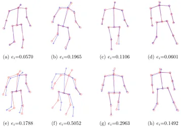
(a) ei=0.0570 (b) ei=0.1965 (c) ei=0.1106 (d)ei=0.0601

[image:42.595.147.505.368.618.2]

(e) ei=0.1788 (f) ei=0.5052 (g) ei=0.2963 (h)ei=0.1492

Figure 3.5: 3D reconstruction results of our method (top row) and PND (bottom row) on UMPM dataset. “◦” indicates ground truth and “+” indicates 3D reconstruction points. Parameters: K = 3, σ = 10. Sequences from left to right: circle, free, table, triangle.

We also conducted experiments on noisy measurements and those with

miss-ing data on UMPM sequences. In the noisy data case, Gaussian noise was added

to the UMPM sequences with a standard deviation of σn = 0.01 max{W} and

Shape Clustering and Spatial temporal Constraint for Non rigid Structure from Motion