A Survey of Convexity Estimates and Singularities for Mean Curvature Flow with Surgery

(1)

A Survey of Convexity Estimates and

Singularities for Mean Curvature Flow

with Surgery

Hugh Cooney

November 2018

A thesis submitted in partial fulfilment of the requirements for the degree of Bachelor of Science (Honours)

(2)

(3)

Declaration

The work in this thesis is my own except where otherwise stated.

(4)

(5)

Acknowledgements

Thank you to my supervisor Ben Andrews for introducing me to such an inter-esting area of mathematics, for all his assistance throughout the year and for being so generous with his time. Thank you also to my professors throughout the year; Pierre Portal, Griff Ware, Joan Licata and Xu-Jia Wang. Thank you also to my Honours cohort, in particular Kyle, Sam, Jane, Adele, Feng and Chris for all their stimulating conversations and jellification achievements. Finally, thank you to my parents for all their support.

(6)

(7)

Abstract

In this survey we aim to introduce the basics of Mean Curvature Flow and detail the programme of Mean Curvature Flow with surgery developed by Huisken and Sinestrari over four seminal papers, [29],[28],[30] and [8]. We divide the survey into 3 chapters, the first being an introduction to the Mean Curvature Flow. This is followed by the convexity estimates that were developed by Huisken and Sinestrari, which allow us to understand the singularities that form under Mean Curvature Flow. We also present an alternative proof of the convexity estimates for compact mean-convex Mean Curvature Flow that avoids the use of induction on symmetric functions and is based off the proof of Ben Andrews, James Mccoy and Mat Langford in [5]. In chapter 3 we use the convexity estimates for the 2-convex case to discuss the surgery procedure. We also compare and contrast aspects of the Ricci Flow and Hamilton’s surgery programme for 4 dimensional manifolds with Positive Isotropic Curvature undergoing Ricci Flow which moti-vated Huisken and Sinestrari’s surgery procedure. In this chapter we explain too the added technicality that was required to extend Mean Curvature Flow with surgery to dimensionn = 2, achieved in [8], and we relate it to Perelman’s surgery programme that extended Ricci Flow to 3-manifolds. Finally, we conclude with some topological applications and a discussion of further open problems.

(8)

(9)

Chapter 1 Background Material

1.1 Preliminaries

We will assume the reader is familiar with the standard results of Differenetial Geometry and PDE’s throughout this survey. For a background on these subjects we refer to the textbook by Evans [15], and Do Carmo’s textbook [16]. However for the reader’s convenience we recall some basic definitions and results concerning differential geometry and hypersurfaces.

We begin with a discussion on some of the different types of curvature. Re-call that an immersed submanifold of _RN _{is a differentiable manifold} _M _{and an}

immersion X : M → _RN_{. When} _M _{is of dimension} _N ₋_{1 we refer to} _M _{as a}

hypersurface.

Definition 1.1 (Weingarten Map). The smooth mapping W :M →_Sn_⊂

Rn+1 defined byW (ξ)(p) = −(DξN)(p), wherep∈M,N is the unit normal (toX(M)

at p) and ξp ∈TpM, is called theWeingarten map.

Definition 1.2. For anyξ, η ∈TpM, we define the second fundamental form as

a symmetric bilinear form h(ξ, η) =hWξ, ηi and is a tensor of type (2,0).

Since h is symmetric, we can diagonalize it (with respect to the metric g) and find a basise1, ..., en ofTpM and real numbers κ1, ..., κnsuch that h(ei, x) = κig(ei, x) for all vectors x ∈ TpM. Then we refer to (κi)ni=1 as the principal curvatures of M at the point p and are the eigenvalues of the Weingarten map. Furthermore the mean curvature H is the trace of h, i.e. H :=gij_h

ij.

Remark. The mean curvature is often defined as the average of the principal curvatures, but for our context the mean curvature will be viewed as the sum of

(12)

12 CHAPTER 1. BACKGROUND MATERIAL the principal curvatures

H =

n

X

i=1

κi.

By convention we will denote the mean curvature vector as

~

H =−HN.

The above notions of curvature are termed extrinsic curvatures as they depend on the immersion of a manifold. For Mean Curvature Flow we will always be dealing with hypersurfaces that are immersed into Euclidean space. We will however also want to deal with intrinsic forms of curvature that are computed directly on the manifold using the metric g.

Definition 1.3. For tangent vectors X, Y, the (4,0) tensor given in terms of the Riemman connections by R(X, Y)Z = ∇Y∇XZ = ∇X∇YZ +∇[X,Y]Z is termed the Reimann Curvature Tensor, or simply the curvature tensor. The

Ricci Curvature Rij is given by the trace of the curvature tensor, that is Rij := gkm_R

kijm.

We will require one other notion of curvature which we refer to as the PIC condition:

Definition 1.4. A Riemannian manifold Mn of dimension at least 4 is said to have positive isotropic curvature (PIC) if for every orthonormal 4-frame the curvature tensor satisfies:

R1313+R1414+R2323+R2424 −2R1234 ≥0 (1.1) In Riemannian Geometry there is in fact an important link between the in-trinsic notion of curvature and exin-trinsic curvature given by the Gauss-Codazzi equations. For a hypersurface in _Rn the equations are given as follows

Rijkl =hikhjl−hjkhil (1.2)

and

∇ihjk =∇jhik. (1.3)

Gauss-weingarten equations:

∂X2 ∂xi∂xj

= Γk_ij∂X

∂xk

+hijN, ∂N ∂xj

=−hjlgls ∂X ∂xs

. (1.4)

Simon’s identity

(13)

1.2. INTRODUCTION TO MEAN CURVATURE FLOW 13

1.2 Introduction to Mean Curvature Flow

Mean Curvature Flow (MCF) is an extrinsic geometric flow which evolves hyper-surfaces in the direction of the unit normal with speed given by the mean curva-ture at each point. The Mean Curvacurva-ture Flow was first proposed by Mullins in [36] as a model for the formation of grain boundaries in annealing metals however due to its many interesting characteristics the geometric properties of MCF have been studied extensively and have found applications in other areas of mathe-matics and physics. MCF is also a good candidate to model soap film as they are known to converge to minimal surfaces which are critical points of the MCF and their motion is determined by surface tension which is directly proportional to their curvature. This leads to MCF having many applications in materials sci-ence and image processing. We describe the Mean Curvature Flow by a system of weakly parabolic partial differential equations for the locally embedded map of the evolving hypersurfaces.

Definition 1.5 (Mean Curvature Flow). We say that a smooth family of n -dimensional hypersurfaces (Mt)t∈I immersed in Rn+1 moves by Mean Curvature

Flow if there is a one-parameter family Xt = X(·, t) of immersions with

corre-sponding images

Mt =Xt(M) such that ∂X

∂t (p, t) = −H(p, t)N(p, t), p∈M, t≥0, (1.6)

X(·,0) = X0, (1.7)

is satisfied for some initial data X0 and where H(p, t) and N(p, t) are the mean curvature and outer normal at a point p∈M respectively.

(14)

14 CHAPTER 1. BACKGROUND MATERIAL with the Ricci Flow (see Definition 1.8). For Ricci Flow with positive curvature operator (see equation 3.4) Hamilton proved a matrix Harnack inequality and was later proved in an alternate way by Bennet Chow based on discussions with Hamilton in [12]. Meanwhile Perelman’s Entropy Formula used in [38] can also be viewed as an analogue of Huisken’s monotonicity formula and suggests under certain constraints singularities of the Ricci Flow are modelled by shrinking soli-tons. While there is no way, that the author is aware of, of transforming one flow into the other, their similarities have meant that much of the programme of MCF and Ricci Flow has developed simultaneously. For example the Harnack inequal-ity for Ricci Flow was motivated by Hamilton’s proof of the Harnack estimates of MCF in [21] and the surgery programme of Huisken and Sinestrari for MCF in [30] which we explore in chapter 3 is motivated by Hamilton’s pioneering of Ricci Flow with surgery on 4-manifolds in [19].

We can also show that ∆g(t)X(p, t)−H~(p, t) = 0, where ∆g(t) is the Laplace-Beltrami operator on M associated to the metric g(t) and induced by the im-mersion Xt.

short time existence Even though MCF can be written as a Laplacian which is an elliptic operator, the PDE does not enjoy the standard existence results as it is not a strictly parabolic PDE due to its invariance under diffemoprhism. Fortunately MCF does enjoy short time existence and uniqueness. Put more formally

Theorem 1.1. Let X0 : M → Rn+1 be an immersion of a compact manifold M. Then there exists a positive constant T > 0 and a unique smooth family of immersions Xt for t∈[0, T] that satisfy equation 1.6.

There have been multiple proofs over the years of short time existence for the flow. We refer the reader to [9] where the Deturk trick is used to prove short time existence i.e by coupling the flow with a similar flow that avoids the diffeomorphism invariance. The same technique was used by Deturk in the Ricci Flow case and a more detailed explanation can be found in [2].

1.3 Notable examples

(15)

1.3. NOTABLE EXAMPLES 15 plane, this case is much simpler to visualise. An important feature of CSF is the following theorem:

Theorem 1.2 (Gage-Hamilton-Grayson Theorem). If a closed embedded curve moves by curve shortening flow, then it will remain embedded, and it will become convex in finite time.

We reference a very elegant proof of the above theorem by Ben Andrews and Paul Bryan in [4] that uses a distance comparison technique. Observe also then that under a rescaling the singularities of CSF for closed embedded curves can be characterised by a circle.

Self-similar solutions and translating solitons Another type of solution that is of particular interest for any geometric flow are solutions that retain their geometric shape under the flow up to translation or rescaling.

Definition 1.6. A solution to equation 1.6 is calledself-similar if H ≡αX⊥, for

α∈_R. A solution of MCF is called a translating soliton if its mean curvature H

and its normal vector N satisfyH ≡ hN, zi for some non-zero z ∈_Rn+1_.

It is clear from the above definition that a self-similar solution retains its ‘shape’ under the flow and when α > 0 the solution expands along the flow, in which case we say it is a self-expander, similarly if α <0 the surface shrinks and we say it is a self-shrinker.

Remark. In the compact case we only need consider self-shrinkers as we can bound the manifold by a sphere, see example 1.2, which contracts to a point in finite time and by the Comparison Principle (see theorem 1.4) we must have that the compact manifold disappears before the sphere does and hence it is not possible for a compact self-similar solution with α≥0 to exist.

The above definitions suggest that there exists solutions to MCF that exist for all time, this brings us to the following definition:

Definition 1.7. A solution of MCF that exists for all time is called an eternal solution, while a solution that exists for all t ∈ (−∞, T) is called an ancient solution.

(16)

16 CHAPTER 1. BACKGROUND MATERIAL

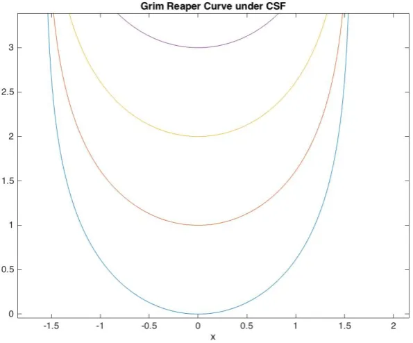
Example 1.1 (Grim Reaper Curve). It is well known [17] that the only trans-lating soliton for CSF is the ‘Grim Reaper’ curve, given by the equation

[image:16.595.111.409.232.479.2]

Γt=−log(cos(x)) +t. (1.8)

Figure 1.1 demonstrates the upwards movement of the curve as it undergoes CSF.

Figure 1.1: Grim Reaper curve moving under CSF.

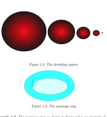
Example 1.2 (Shrinking spheres). The next notable example is the shrinking sphere as seen in figure 1.2. Let Mt = ∂B_ρn₍+1_t₎. Then by the invariance of mean

curvature under isometries equation 1.6 becomes the ODE given by

∂tρ=

−n ρ .

By setting ρ(0) =ρ0 we obtain

ρ(t) =

q

ρ2 0−2nt

(17)

1.3. NOTABLE EXAMPLES 17

[image:17.595.132.503.99.503.2]

Figure 1.2: The shrinking sphere.

Figure 1.3: The marriage ring

(18)

18 CHAPTER 1. BACKGROUND MATERIAL

1.4 Evolution of Geometric Quantities

Proposition 1.1. For future reference it will be important to understand how certain geometric quantities evolve under the flow, hence we provide the following computations.

(i) _∂t∂gij =−2Hhij,

(ii) ∂N_∂t =∇H,

(iii) _∂t∂hij = ∆hij −2Hhilglmhmj +|A|2hij,

(iv) ∂H_∂t = ∆H+|A|2_H_,

(v) ∂|_∂tA|2 = ∆|A|2_{− |∇}_A_|2 _{+ 2|}_A_|4_,

Proof. For (i) recall that the inner product h·,·ion_RN _{induces a metric} _g _which

we can write as follows:

∂tgij = d

dth∂iX, ∂jXig

=h2∂i∂tX, ∂jXig

=h2∂i−HN, ∂jXig

=−2Hh∂iN, ∂jXig

=−2Hhij.

Remark. Similarly we can compute ∂tgij = 2Hhij using the fact that∂tgijgjk = 0

and applying (i). For (ii) observe

∂

∂tN =h ∂ ∂tN,

∂X ∂xi

i∂X

∂xj

gij =hN, ∂ ∂t

∂X ∂xi

i∂X

∂xj gij

= ∂

∂xi

H· ∂X

∂xj

gij =∇H

(19)

1.5. THE MAXIMUM PRINCIPLE AND HUISKEN’S MONOTONICITY FORMULA19

∂ ∂thij =

∂ ∂thN,

∂2_X

∂xi∂xji

=hN,∂

2₍_HN₎

∂xi∂xj

i − h∇H, ∂

2_X

∂xi∂xj

i

= ∂ 2_H

∂xi∂xj

−HhN, ∂ ∂xi

hjlgls∂X ∂xs

i − h ∂

∂xl

H· ∂X

∂xs

gls,Γk_ij∂X

∂xk

+hijNi = ∂

2_H

∂xi∂xj

−HhjlglshN, ∂2_X

∂xi∂xs

−Γk_ij ∂

∂xk H

=∇i∇jH−Hhijglshsj = ∆hij −2Hhilglshsj +|A|2hij

Recall the the mean curvature is the trace of the second fundamental form, i.e.

gijhij =H, then

∂ ∂tH =

∂ ∂t(g

ij

hij) =gij ∂

∂thij + 2Hg ik

gjlhklhij = ∆H+|A|2H.

For the final computation we make use of the following

∆|A|2 =gkl∇k∇l(gpqgmnhpmhqn) = 2gpqgmnhpm∆hqn+ 2|∇A|2. (1.9)

and then combining this with (iii) we can compute

∂t|A|2 =∂t(gikgjlhijhkl) = ∆|A|2− |∇A|2+ 2|A|4.

1.5 The Maximum Principle and Huisken’s

Mono-tonicity Formula

The following definition of the monotonicty formula is taken from [14]. We will denote x=x(p, t) the coordinate vector of the image X(p, t) for a point p∈M. Then for a fixed point (x0, t0) ∈ Rn+1 we define the backward heat kernel ρ =

ρ(x, t) by

ρ(x, t) = (4π(t0−t))−n/2exp

−|xo−x|2

4(t0−t)

, t0 > t, (1.10)

Then an important tool developed by Huisken for studying blow-ups is the mono-tonicity formula.

d dt

Z

Mt

ρdµt =

Z

Mt

ρ

H+

1

2τ(x−x0)

⊥

2

(20)

20 CHAPTER 1. BACKGROUND MATERIAL Where dµt is the measure on Mt. Also for a function φ = φ(x, t) on M the

formula can be written more generally as

d dt

Z

Mt

φρdµt=

Z

Mt

d

dtφ−∆φ

ρdµt−

Z Mt φρ H+ 1

2τ(x−x0)

⊥

2

dµt (1.12)

Then we now prove a Maximum Principle for MCF:

Theorem 1.3. Let (Mt)t∈(t1,t0) be a solution of mean curvature flow consisting

of hypersurfaces Mt = Xt(Mn) where X(·, t) = Xt : Mn → Rn+1 and Mn is

compact. Suppose h : Mn_× _[_t

1, t0) → R is smooth for t > t1, continuous on Mn_×_[_t

1, t0] and satisfies an inequality of the form

d

dt −∆Mt

h≤a· ∇Mt_h. _(1.13)

Then

max

Mn h(·, t)≤max_Mn h(·, t1)

for all t ∈ [t1, t0]. For the vector field a : Mn×[t1, t0) → Rn+1 we only require

that it is well-defined and regular in a neighbourhood of all maximum points of h

and that a0 = sup_M×[0,t1]|a|<∞

The following proof is from [14]

Proof. Let k = sup_M₀h and define hk = max(h −k,0). Then applying the

inequality 1.13 to the term h2

k we see that

d

dt −∆Mt

h2_k ≤2hka· ∇hk−2|∇hk|2.

Applying Young’s inequality we obtain

d

dt −∆

h2_k≤ 1 2a

2 0h2k.

Now applying Huisken’s monotonicity formula we see that

d dt

Z

h2_kρdµt ≤

1 2a

2 0

Z

h2_kρdµt

which completes the proof.

(21)

1.6. RICCI FLOW 21 the evolution of the mean curvature we see that d

dtφ≤2φ

2_{, where}_φ _{= max}

Mt|A| 2_, yielding the estimate

max

Mt

|A|2 _≥ 1 2(T −t),

So it is natural to consider 2 types of singularities, the first where there exists a constant c0 such that maxMt|A|

2 _≤ c0

(T−t) and the second where there does not. We refer to these as type-I and type-II singularities respectively.

Mean Curvature Flow also enjoys a comparison Principle:

Theorem 1.4. Let X : M1 × [0, T[→ _Rn+1 _and _F _: _M2 _× _[0_{, T}_[→

Rn+1 be

two hypersurfaces moving by MCF. Suppose also that M1 is compact. Then the distance between them is non-decreasing in time.

From the above theorem it is clear that if M2 is embedded in M1 and M1 compact. Then M2 remains inside M1 for all time t ∈ [0, T[. A proof of the comparison theorem can be found in Theorem 2.2.1 of [34].

1.6 Ricci Flow

While the primary focus of this paper is the Mean Curvature Flow, MCF has many similarities with the intrinsic geometric flow, the Ricci Flow. In fact the surgery argument which we present in chapter 3 and which was developed by Huisken and Sinestrari in [30] is in fact based on the prior work of Hamilton in [19] in constructing a similar surgery procedure for the Ricci Flow.

Definition 1.8 (Ricci Flow). The Ricci Flow is family of manifolds (Mt, gt) that

is evolved by a quasi-linear (weakly) parabolic PDE on an initial metric g0 of a smooth Riemannian manifold M0 given by the following equation

∂

∂tgij =−2Ricij (1.14)

For more information concerning the Ricci Flow we refer the reader to Bennett Chow and Dan Knopf’s book [11]. From Proposition 1.1 we know how the metric evolves under MCF, then combining this with the Gauss-Codazzi equations 1.2 and recalling that the Ricci Curvature is the trace of the curvature tensor we obtain the following

Rij =Rkkij =gkmRkijm =gkmhkmhij −gkmhkjhim

(22)

22 CHAPTER 1. BACKGROUND MATERIAL and therefore the evolution of the metric under the mean curvature flow becomes

∂tgij =−2Rij + 2gkmhkjhim

(23)

Chapter 2 Asymptotic behaviour of

singularities

The central aim of this survey is to understand Huisken and Sinestrari’s surgery programme for MCF which will allow one, by hand, to go in and remove regions of high curvature so as to avoid the formation of singularities and hence develop a way of flowing through singular times. In order to develop such a surgery algorithm for Mean Curvature Flow we first must understand the singularities that form. Throughout the literature there has been a broad number of results attempting to classify solutions of Mean Curvature Flow and its behaviour near singular times. We have seen that in the case n= 1 Grayson’s Theorem provides us with a very nice classification of curves undergoing curve shortening flow. While there is no analogous result in higher dimension there is the famous 1984 result by Huisken [26] for compact convex surfaces converging to spheres.

Theorem 2.1 (Hui1984). Let n≥2 and assume M0 is uniformly convex. Then the mean curvature flow exists for finite time and the hypersurface Mt converges

to a single point. Also under a rescaling, the solutions to the normalised mean curvature flow converge to a sphere of area |M0| in the C∞-topology.

Recall the shrinking sphere example 1.2 and the Comparison Principle meant initial hypersurfaces that were closed and compact contracted in finite time and therefore had to develop a singularity. However in general understanding the formation of singularities in higher dimensions or in the non-compact case is much more difficult. This brings us to the work of Ecker and Huisken in [14] who were able to classify the solutions when they can be written as entire graphs.

(24)

24 CHAPTER 2. ASYMPTOTIC BEHAVIOUR OF SINGULARITIES

2.1 Entire Graphs

Let us know to restrict our attention to Mean Curvature Flow of entire graphs, so our hypersurfaces are of the form Mt= graph u(·, t) foru(·, t) :Rn→R, that

is we assume that the last component of the embedding Xt = (X·, t) for Mt can

be expressed as a function of the first n-components, i.e.

Xn+1(p, t) = u( ˆX(p, t), t).

Then the unit normal vector field to a hypersurface M = graphu is given by

N = _p(−Du,1) 1 +|Du|2, the mean curvature is given by

H =−div_p Du

1 +|Du|2,

.

Then by equation 1.6 we obtain evolution equation for MCF of entire graphs

∂u ∂t =

p

1 +|Du|2_div Du

p

1 +|Du|2

. (2.1)

In [14] an elegant classification of solutions in the case for entire graphs was obtained. Note that unless stated otherwise the following results are from [14].

Being able to write M as an entire graph implies that there exists a unit vector ω ∈_Rn+1 _{such that for any unit normal} _N _of _M _{we have}

hN, ωi>0 everywhere on M.

We first want to ensure that Mt remains a graph for all t ≥0, to do this we

need to estimate the quantityhN, ωifrom below, which is equivalent to estimating 1

hN, ωi =:v

from above. Let A = {hij} be the second fundamental form, {ei}1≤i≤n on M

be a local orthonormal frame. Then we denote the quantity u = hx, ωi the ‘height’ of M with respect to the hyperplane orthogonal to ω, and it follows that ∇u=hei, ωiei.

Lemma 2.1. The quantity v satisfies

d

dt −∆

v =−|A|2_v₋ 2|∇v| 2

(25)

2.1. ENTIRE GRAPHS 25

Proof. From Proposition 1.1 (ii)

d

dtv =−v

2_h∇_{H, ω}_i_. Then computing the second term

∆v =ei −v2h∇eiN, ωi

=ei −v2hhilel, ωi

=−v2h∇H, ωi+v|A|2+ 2v−1|∇v|2.

Theorem 2.2. Ifv is bounded at initial time by some constantC, then it remains bounded by C.

The proof of which follows by applying a parabolic maximum principle ar-gument to the above quantity (see Theorem 5.1 in [14]). From now on we shall derive results by considering the case of linear growth, that is for some fixed constant c1 ≥1, the inequality

v ≤c1, (2.2)

holds everywhere on M. Theorem 2.2 then ensures that the above inequality remains valid for all t >0.

To guarantee longtime existence of a solution for the Mean Curvature Flow, we must obtain a priori bounds for the second fundamental form on M. Ecker and Huisken then derive estimates interior in time which allows us to prove existence of a longtime smooth solution to MCF with ‘rough’ (Lipschitz) initial data. We begin with the following results which are relatively straightforward yet lengthy computations so we refer the reader to (4.1-4.3) in Ecker and Huisken’s paper [14].

Lemma 2.2. The curvature satisfies the following inequality

d

dt −∆

|A|2_v2 _{≤ −2}_v−1_∇_v_{· ∇(|}_A_|2_v2₎_.

Corollary 2.1. If Mt is a smooth solution of (1) with bounded gradient and

bounded curvature on each Mt, then there is the a priori estimate

sup

Mt

|A|2v2 ≤sup

M0

|A|2v2.

(26)

Lemma 2.3. IfM, is a smooth solution of 1.6 such thatv,|A|2_,_|∇_A_|2_{, ...,}_|∇m_A_|2

are bounded on each Mt, then we have for all t≥0 the a priori estimate

sup

Mt

|∇m_A_{| ≤}_C₍_m₎

where C(m) only depends on m, n, c, and sup_M₀|∇j_A_| _for ₀_≤_j _≤_m_.

We now derive estimates interior in time for the curvature and all its deriva-tives.

Proposition 2.1. Let M, be a smooth solution of (1.6) satisfying the linear growth condition. Then for each m≥0 there is a constantC(m) depending only on c1, n and m such that

tm+1|∇mA|2 ≤C(m), (2.3) holds uniformly on Mt.

Proof. We will prove the case for m=0, form >0 the proposition can be proved by induction and we refer the reader again to Ecker and Huisken’s paper proposition 4.4.

From our previous computations we compute

d

dt −∆

(2t|A|2_v2₊_v2₎_{≤ −2}_v−1_∇_v _{· ∇(2}_t_|_A_|2_v2₎₋_6|∇_v_|2 ≤ −2v−1∇v · ∇(2t|A|2_v2₊_v2₎_. Then applying the weak maximum principle we see that the estimate

2t|A|2_v2₊_v2 _≤_c2 1

Holds uniformly onMt, and hence proves the interior estimate for the casem = 0.

Using this proposition we can now prove existence of longtime solutions for ‘rough’ (Lipschitz) initial data.

Theorem 2.3. If the initial hypersurfaceM0 is Lipschitz continuous and satisfies

sup

M0

v ≤c1,

(27)

Proof. We first consider the case that the initial hypersurface is smooth with sup_M

0|∇

m_A_| _{is bounded for all} _m _≥ _{0. Recall our equation for the evolution of}

entire graphs we first set

F(u) :=δij −

∂iu∂ju

1 +|∇u|2

∂i∂ju (2.4)

so our quasi-linear equation can be restated as

∂tu+F(u) = 0, u(0) =u0

The mapping F is real analytic. We can then consider the linearisation of our quasi-linear equation for MCF of graphs;

∂tv+F0(u)v =f, v(0) = v0

where F0(u) is the Frechet derivative of F at u . Then our linearised equation enjoys the property of maximal regularity so in view of the bound on v the linearised equation is a uniformly parabolic equation and the Implicit Function Theorem guarantees the existence of a unique smooth solution on some short time interval. Our uniforma priori estimates in Proposition 2.1 then ensure that this solution extends to all t > 0. But since our estimates were all interior in time by approximation we get long time existence for Lipschitz initial data.

In fact Ecker and Huisken then use this longtime existence to study the be-haviour of solutionsMtfor large times in the case of linear growth. By a rescaling

Ecker and Huisken found that as t → ∞ the limiting solution ˜M∞ satisfies the

equation

F⊥ =H.

From Proposition 2.1 it should be clear that solutions ‘flatten out’ as t→ ∞.

Theorem 2.4. If M is an entire graph of at most polynomial growth satisfying

H =hx, Ni,

then M is a plane. Proof. We compute

∆v =|A|2_v _{+ 2}_v−1_|∇_v_|2₊_h_{x, e}

ii∇iv.

multiplying thus equation by ρ = exp(−|₂x|2) and then integrating by parts gives us

Z

M

|A|2_vρdµ_{+ 2}

Z

M

(28)

28 CHAPTER 2. ASYMPTOTIC BEHAVIOUR OF SINGULARITIES Then applying Proposition 2.1 we conclude that the second fundamental form must go to zero and hence M converges to a flat plane.

In fact more recently in [31] by Koch and Lamm, it is shown that solutions can also be constructed for entire graphs in the higher co-dimensional case that also enjoy existence and uniqueness. That is f :_Rn×[0,∞)→_Rm

∂tf =gij ∂2_f

∂xi∂xj

, f(·,0) =f0, (2.5)

where gij ₌_δ

ij +h_∂x∂f

i,

∂f

∂xji. Then for m= 1 we calculate

gij =δij−

∇if∇jf

1 +|∇f|2

and therefore we recover our equation for the mean curvature flow for graphs in codimension 1, i.e.

∂tf =

p

1 +|∇f|2_div ∇f

p

1 +|∇f|2

.

Theorem 2.5. There exists ε >0, C > 0 such that for every map f0 :Rn→Rm

satisfying ||f0||C0,1₍

Rn,Rm) < ε there exists a global analytic solution f ∈X∞of(1) and ||f||X∞ ≤C||f0||C0,1₍

Rn,Rm). The solution is unique in the ball B

X∞₍₀_{, C} ε) =

{f | ||f||X∞ ≤Cε}.

The proof follows from the same arguments used by Koch and Lamm [31] for the Willmore flow though we should note that scaling invariance is given by

fλ(x, t) =

1

λf(λx, λ

2_t₎_. And we rewrite the parabolic system as

d

dt −∆

f = (gij −δij) ∂2_f

∂xi∂xj

=:M[f].

To understand why the case of m > 1 is much more technical then the Ecker Huisken result for m= 1 we note an example given by [33]

Theorem 2.6. The Lipschitz function f :_R4 →_R3 _{given by}

f(x) = √

5 2 ||x||η

x

||x||

x6= 0,

(29)

Remark. There are also analogous results from _R7 _to

R4. This shows that there exists a Lipschitz continuous minimal graph that is not in the class of C1_{. By} constructing a stable minimal cone in R7 _{that is a Lipschitz graph over} _R4 _we see that we won’t get the same regularity results as Ecker-Huisken and instead require a smallness condition on the Lipschitz norm of the initial data as minimal submanifolds are a stationary phase of the mean curvature flow.

In [42] such a bound is found.

Theorem 2.7. LetMn_{be a compact Lipschitz submanifold of}

Rn+m. There exists

a positive constantK depending on n andm such that if Mn _{satisfies the} _K _local

Lipschitz condition, then the mean curvature flow of Mn _{has a smooth solution}

on some time interval (0, T].

Contrasting the existence and uniqueness results for Mean Curvature Flow of graphs in the Koch-Lamm paper with the case for Willmore flow of graphs in the same paper it was remarked that the necessity of the smallness assumption on the initial data was an open problem however in light of the above result it is clear that the smallness assumption is a necessary condition for Mean Curvature Flow of graphs in the case of co-dimension greater than 1. Finally an interesting result due to Koch-Lamm is the characterisation of self-similar solutions to the Mean Curvature Flow.

Corollary 2.2. There exists ε > 0, C > 0 such that if f0 ∈ C(0,1)(Rn,Rm) is

self-similar f0(x) = a_λf0(λx)for every x∈Rn with ||f0||C0,1₍

Rn,Rm)< ε then there exists an analytic, self-similar solution f ∈X∞ of the mean curvature flow which

satisfies the estimates ||f||X∞ ≤ C||f0||C0,1₍

Rn,Rm). The solution is unique in the ball BX∞₍₀_{, C}

ε).

Proof. We consider self-similar initial data f0, i.e. f0 which satisfy

f0(x) = 1

λf0(λx) λ >0 x∈R n

HenceM0 = graph(f0) is a cone with vertex 0. If we assume that||f0||C0,1₍

Rn,Rm) <

ε, where ε is as in the previous theorem. Then applying Theorem 5.1 of [31] we get existence and uniqueness of an analytic solutionf ∈X∞with initial condition

f(·,0) = f0.

Now define f0,λ(x, t) = 1_λf0(λ(x)), then ||f0,λ||C0,1₍

Rn) = ||f0||C0,1(Rn) < ε and

hencefλ(x, t) = 1_λf(λx, λ2t) is the unique analytic solution of MCF inX∞(where

(30)

30 CHAPTER 2. ASYMPTOTIC BEHAVIOUR OF SINGULARITIES that for any self-similar initial dataf0 with ||f0||C0,1₍

Rn)< εthere exists a unique analytic solution of MCF which satisfies

f(x, t) = 1

λf(λx, λ

2_t₎_,

x∈_R, t >0, λ >0.

2.2 Convexity estimates (Mean-Convex, n=2)

The first of the four seminal papers of Huisken and Sinestrari that we explore is developing convexity estimates for the case of non-negative mean curvature which is referred to as mean-convex. We examine the 1999 paper [28] that gives a classification of the possible singular behaviour for mean convex surfaces in the case n = 2.

The convexity estimates established here will form the basis for understanding singular behaviour of the flow in higher dimensional cases and which we will then use in chapter 3 to explain the surgery procedure.

In the following section we will be considering Mean Curvature Flows that are smooth, compact, mean-convex of dimension n ≥ 2 and without boundary, and we will classify the limiting surfaces that are obtained for both type I and type II singularities. From [26] Theorem 8.1 we know that there exists a smooth solution for this problem up to some critical time T < ∞ and satisfies

T ≤ (diamM0) 2

8n (2.6)

We first begin with some relevant results and lemmas that will be used later in the proof of Theorem 2.8. Proofs for all the below results can be found in [28].

Let us now introduce, for η∈_R and σ ∈[0,2], the function

gσ,η =

|A|2 ₋_{(1 +}_η₎_H2

H2−σ (2.7)

Then we can compute from the evolution equations in Proposition 1.1

∂gσ,η

∂t = ∆gσ,η+

2(1−σ)

H h∇H,∇gσ,ηi −

σ(1−σ)

H2 gσ,η|∇H| 2

− 2

H4−σ|H∇ihkl− ∇iHhkl|

2₊_σ_|_A_|2_g

σ,η.

By setting σ= 0 we obtain

∂ ∂t

|A|2

H2 = ∆ |A|2

H2 + 2

Hh∇H,∇

|A|2

H2 i − 2

H4|H∇ihkl− ∇iHhkl|

(31)

2.2. CONVEXITY ESTIMATES (MEAN-CONVEX, N=2) 31

Remark. Where clear we will write gσ,η =g for fixed η, σ, and g+ to denote the positive part of g.

By the maximum principle and by the compactness of M we obtain that |A|2_/H2 _{is uniformly bounded from above by its initial data. Thus, if we call} _c

0 the maximum of |A|2_/H2 _on _M0 _{, we have}

|A|2 _≤_c

0H2. (2.9)

Lemma 2.4. There exists constants c2, c3 such that

d dt

Z

Mt

gp₊dµ≤p(p−1) 2

Z

Mt

gp₊−2|∇g|2_dµ₋ p

c3

Z

Mt

g₊p−1 H2−σ|∇H|

2_dµ

−p

Z

Mt

gp₊−1

2_dµ₊_pσ

Z

Mt |A|2_gp

+dµ

for any p≥c2.

Proposition 2.2. [Proposition 3.6 [28]] Given η ∈ (0,1), there exists constants

c4, c5, such that the Lp(M) norm of (gσ,η)+ is a non-increasing function of t for any p, σ such that

p≥c4, σ ≤(c5p)−1/2.

We can now present the proof of the key convexity estimate of Huisken and Sinestrari for mean-convex hypersurfaces of dimension n= 2.

Theorem 2.8. Let Mt , t ∈ [0, T) be a smooth solution of the mean curvature

flow, with n ≥ 2 and the initial manifold M0 compact and of positive mean curvature. Then for any η >0 there exists constants Cη > 0 depending only on

n, η and M0 such that

R ≥ −ηH2−Cη

on Mt for any t∈[0, T).

Proof. Using the Lp_{-estimate of the previous proposition we aim to derive a}

uni-form bound on the supremum of gσ,η. To do this set k0 = sup

σ∈[0,1] sup

M0

g,

then given any k ≥k0, set

v = (gσ,η−k) p/2

(32)

32 CHAPTER 2. ASYMPTOTIC BEHAVIOUR OF SINGULARITIES Then using Lemma 2.4 and (2.8) we compute

d dt

Z

v2dµ=

Z _∂

∂t(gσ,η−k)

p(gσ,η−k)p

−1 + −H2

dµ

=p

Z

∆gσ,η(gσ,η−k)p

−1

+ + 2p(1−σ)

Z

(gσ,η −k) p−1 +

H h∇H,∇gσ,ηi

−pσ(1−σ)

Z

gσ,η(gσ,η −k)p₊−1

H2 |∇H|

2

−

Z ₂_p

2 +σp

Z

|A|2gp_σ,η(gσ,η−k)p₊−1 ≤ −p(p−1)

2

Z

g₊p−2|∇gσ,η|2dµ+σp

Z

|A|2g_σ,ηp dµ

Then, using the fact that on A(k, t) we have 1/2p(p−1)g₊p−2|∇g|2 _{≥ |∇}_gp/2_|2_{, we} can write

d dt

Z

v2dµ+

Z

|∇v|2_dµ_≤_σpc 0

Z

H2g_σ,ηp dµ. (2.10) On the other hand we have the following Sobolev-type inequality of Simon and Michael (see [35]) that is valid for any Lipschitz function on Mt

Z

v2qdµ

1/q

≤c6

Z

|∇v|2_dµ₊_c 6

Z

A(k,t)

Hndµ

2/nZ

v2qdµ

1/q

. (2.11)

Here q = n/(n−2) if n > 2 and an arbitrary number greater than 1 if n = 2. Now observe that, if

p≥max{c4,4n2c5}, σ ≤(4c5p)−1/2 then we have

Z

Mt

Hngp_σ,ηdµ=

Z

Mt

g_σp0_,ηdµ

with

σ0 =σ+ n

p ≤

1 2√c5p

+√1

p n √ p ≤ 1 √

c5p

.

Thus by Proposition 2.2 we can show that the Lp_{-norms of} _g

σ,η are bounded,

provided σ is sufficiently small,

Z

A(k,t)

Hndµ2/n ≤k−2p/n

Z

A(k,t)

Hngp_σ,ηdµ2/n

≤k−2p/n

Z

M0

gp_σ0_,ηdµ

2/n

≤(1 +|M0|)k0

k

(33)

2.2. CONVEXITY ESTIMATES (MEAN-CONVEX, N=2) 33 Therefore we can then fix k1 > k0 large enough such that for any k ≥k0 we may absorb the last term in 2.11 and then exploit the |∇v| term in 2.10 to obtain

d dt

Z

v2dµ+ 1

c7

Z

v2qdµ

1/q

≤c0pσ

Z

A(k,t)

H2g_σ,ηp dµ, (2.12)

where we choose c7 such that _c1₇ ≥ _c1₆ −

R

A(k,t)H

n_dµ2/n

. Then denoting any constant that depends on n,cn and integrating (2.12) over time gives

sup [0,T)

Z

A(k,t)

v2dµ+cn

Z T

0

Z

A(k,t)

v2qdµ1/qdt ≤σp

Z T

0

Z

A(k,t)

H2g_σ,ηp dµdt.

Now using interpolation inequalities for Lp_-spaces

Z

A(k,t)

v2q0_dµ

1/q0

≤

Z

A(k,t)

v2qdµ a/qZ

A(k,t)

v2dµ

(1−a)

,

1

q0 = a

q + (1−a),

with a= 1/q0 such that 1 < q0 < q. Then we have

Z T

0

Z

A(k,t)

v2q0_dµdt

1/q0

≤cnσp

Z T

0

Z

A(k,t)

H2gp_σ,ηdµdt

≤cnσp

Z T

0

Z

A(k,t)

dµdt

1−1/rZ T

0

Z

A(k,t)

H2rg_σ,ηprdµdt

1/r ,

where r >1. Then applying H¨older’s Inequality observe that

Z T

0

Z

A(k,t)

vpdµdt≤c8σp

Z T

0

Z

A(k,t)

dµdt

1+b−1/rZ T

0

Z

A(k,t)

H2rg_σ,ηprdµdt

1/r ,

where b = (q−1)/(2q−1). Let us now choose r large enough such that γ := 1 +b−1/r > 1. Then we can estimate the second factor on the right hand side provided p, σ−1 _{are larger than suitable constants depending only on} _{n, η,}M0_. And so we obtain a constant c9 such that for allh > k ≥k1

|h−k|p

Z T

0

Z

A(h,t

dµdt≤

Z T

0

Z

A(k,t)

vpdµdt

≤cp₉σp

Z T

0

Z

A(k,t)

dµdt

γ

.

By the Stampacchia Lemma (see Lemma 2.5) we conclude

Z T

0

Z

A(k,t)

(34)

34 CHAPTER 2. ASYMPTOTIC BEHAVIOUR OF SINGULARITIES where

d=cp₉σp2pγ/(γ−1)

Z T

0

Z

A(k,t)

dµdt γ−1

.

Here we use the properties that the critical time T is finite and that the area of Mt decreases with t. We obtain, by the definition of A(k, t),

|A|2 _≤_{(1 +}_η₎_H2 _{= (}_k

1+d1/p)H2−σ. This implies that

|A|2 _≤_{(1 + 2}_η₎_H2₊_K

η

for some Kη depending only on η, n,M0. Setting Cη = Kη/2 we conclude that |A|2 ₋_H2 _≤_ηH2₊_C

η and hence we obtain that R ≥ −ηH2−Cη,

which proves the theorem.

We can now examine the asymptotic behaviour of solutions near singularities. In this regard it helps to consider separately the type I and type II singularities.

Remark. In Hamilton’s paper [20] on the formation of singularities of the Ricci flow classification of type I, II and III singularities are discussed by examining dilations of the flow. With appropriate curvature bounds and bounds on the injectivity radius, it is noted that a limit of the flow can be extracted and that this limit is also a solution of the Ricci flow and converges to a singularity model in the same type. From this argument we are motivated to try and apply the same line of reasoning to the Mean Curvature Flow case.

We then define the dilated flow as in [28] by choosing a sequence (pj, tj) such

that for any integer j ≥1 let tj ∈[0, T −1/j], pj ∈M such that H2(pj, tj)(T −

1

j −tj) = max1≤T−1/jH

2

(p, t)(T − 1

j −t) (2.13)

Keeping the notation consistent with [28] we set

Lj =H(pj, tj), α=−Lj2tj, ωj =L2j(T −tj −

1

j). (2.14)

We note also that tj →T,Lj → ∞and ωj → ∞ inj. Then forj ≥1 the family

of surfaces Mj,τ we wish to consider are defined by the immersions

Xj(·, τ) = Lj(X(·, L−j2τ+tj)−X(pj, tj)) τ ∈[αj, ωj]. (2.15)

Then we denote Aj, Hj as the second fundamental form and the mean curvature

(35)

2.2. CONVEXITY ESTIMATES (MEAN-CONVEX, N=2) 35

Theorem 2.9. Let Mt, t ∈ [0, T) be a smooth solution of the mean curvature

flow, with n≥2. Assume that the initial manifoldM0 is compact and of positive mean curvature. If the flow develops a singularity of type I then a subsequence of the flows Mj,τ converges smoothly to a mean curvature flow gM_τ defined in the

open interval τ ∈(−∞, C).

Otherwise if the flow develops a singularity of type II as t→T, then a subse-quence of the flowsMj,τ converges smoothly to a mean curvature flowMg_τ defined

for τ ∈ _R. The mean curvature He of the limit flow satisfies 0 < He ≤ 1 and is

equal to 1 at least at one point. Furthermore, either Mg_τ has positive scalar

cur-vature everywhere or (up to rigid motion) Mfτ =Rn−1×Γ¯τ, where Γ¯τ is the“grim

reaper” curve given by x=−lncos(y+τ).

For brevity we will only prove the case for type II singularities as for type I singularities the monotonicity formula can be used and a detailed proof can be found in [27]. We also note that in Theorem 5.1 in [27] it is shown that the limiting hypersurface with non-negative mean curvature is eitherSn, Sn−m×_Rm_,_Γ×

Rn−1 and hence the limiting flow having non-negative scalar curvature is immediate. The proof is sketched in [28] so we fill in the remaining details.

Proof. First observe that from Theorem 2.8 we have bounds on Ak and all of

its covariant derivatives. Hence we can apply a method of the Aerzel`a-Ascoli Theorem for submanifolds (see [40]) to obtain a subsequenceMji,τ that converges uniformly on compact subsets of _Rn+1 _×

R to a limiting flow Mfτ such that its

mean curvature satisfies He ≤ 1. Now choosepj to be the origin, translate tj to

zero, then rescale the solution by dilating time by a factor of λ2 _{and space by} _λ and so 0∈Mj,0 for anyj andHj becomes 1. AsMfτ is the limit of hypersurfaces

with positive mean curvature, the limit flow must satisfyHe ≥0. But asHe is not

identically zero and must satisfy the evolution equation given in Proposition 1.1, by the Maximum Principle we infer thatHe is in fact strictly positive everywhere.

Now note that from the definition ofXj, the second fundamental form satisfies Aj(p, τ) =L−j1A(p, L

−2

j τ+tj)

and so combining this with Theorem 2.8 we see that for anyη >0 there exists a constant Cη such that

|Aj|2 ≤(1 +η)Hj2 +CηL−j2

and so we must have that |fA|

2

≤ |fH|

2

. Then again we apply the maximum principle to the evolution equation of _∂t∂ |_HA|22, see

f

|A|2 <|fH|

2

(36)

36 CHAPTER 2. ASYMPTOTIC BEHAVIOUR OF SINGULARITIES in which case we conclude that the limiting hypersurface has positive scalar cur-vature. Otherwise,

f

|A|2 ≡|fH|

2

, |He∇_ihf_kl− ∇_iHehf_kl|2 ≡0. (2.16)

To show that this then implies that Mτf = Rn−1 ×Γ¯τ we aim to employ the

Frobenius theorem. First let e1, e2, N be an adopted orthonormal frame such that H~ =−HN. If we choosee1 = _|∇∇H_H_| then

|∇H|2 _|_A_|2₋

n

X

k=1

h2₁_k

!

≡0,

such that at any given point |∇H| = 0 or |A|2 ₌ Pn

1kh

2

1k. We only need to

consider the second case as otherwise we would have |∇A|2 _{= 0 everywhere. So} suppose there is p0 ∈ M such that |∇H| 6= 0 , then it follows that |A|2 = H2 everywhere. Now choose a sufficiently small neighbourhoodU centred atp0 where ∇H 6= 0. Then since M is analytic we just have to show that U is locally the required hypersurface. Consider the distributions

D1 ={X ∈TpM :p∈M, AX =HX},

D2 ={X ∈TpM :p∈M, AX = 0}.

Then to apply Frobenius’ theorem we just have to show D1,D2 are involutive. To show this, let Xp0 ∈D1 and letγ(c) be a curve in M such thatγ(0) = p0. If

X(c) withX(0) = Xp0 is parallel transported along γ then from the assumption

2.16 we see that

d

dc|AX−HX|

2 ₌ 2∇1H

H |AX−HX|

2_,

such that X(c) remains in D1. And so for X, Y vector fields in D1 so too are ∇XY,∇YX and hence the commutator [X, Y] is in D1. We can then repeat this argument for D2 and so we see that these distributions are in fact involutive and hence we can apply Frobenius. Hence there is a local coordinate patch

V ={(x, y1, ..., yn} of M such thatp0 corresponds to the origin and

E(¯y) = {(x, y1, ..., yn−1)∈V :yk = ¯yk, k= 1, ..., n−1}, F(¯y) ={(x, y1, ..., yn−1)∈V :x= ¯x}

(37)

2.3. MEAN CONVEX N ≥3 37 Then as the tangent space decomposition is invariant under parallel transport

f

Mτ splits isometrically toE(0)×F(0) . Now since eachF(¯x) is an n-1 dimensional

plane and E(0) is a strictly convex curve. Hence we see that Mfτ = Rn−1 × Γτ, where Γτ is a convex eternal solution to the mean curvature flow in the

2-dimensional plane. Finally we can apply Theorem 1.3 in Hamilton’s Harnack inequality paper [21] to see that Γτ is in fact a translating soliton and as discussed

in chapter 1 the only translating soliton in the plane is the Grim Reaper Curve.

Remark. Hence we have a classification for the limiting solution of compact mean-convex surfaces with type I or type II singularities. That is if the singularity is type 1 as t → T, then by Theorem 5.1 of [27] which is proved using the mono-tonicity formula, the limiting flow must be one of the homothetically shrinking solutionsS2_,

R×S andR×Γ, where Γ is one of the self-similar immersed curves introduced by Mullins [36]. Otherwise if the singularity is of type II, then the lim-iting flow is either a strictly convex translating soliton or the translating solution given by_R×Γ¯τ, where ¯Γτ is the “grim reaper” curve given byx=−lncos(y+τ).

2.3 Mean convex

n

≥

3

In the second paper [29], Huisken and Sinestrari extend their classification of singularities of mean convex surfaces to the n dimensional case. To avoid the technical complexities of induction on symmetric functions of curvature used in the Huisken-Sinestrari paper we instead adapt the work done by Ben Andrews, Mat Langford and James McCoy in [5] who work with a carefully constructed curvature pinching function and the use of Stampacchia’s Lemma. We remark that in this paper, the result is found for a more general function defined on the principal curvatures under certain requirements, however we will only be interested in the case of mean curvature which makes many of the calculations much simpler.

Then the main convexity estimate is stated as follows:

Theorem 2.10. Let X :M ×[0, T)→Rn+1 _{be a solution of} ₍₁_.₆₎_{. Then for all}

η >0 there exists a constant Cη >0 such that

κ1 ≥ −ηH(p, t)−Cη (2.17)

(38)

Remark. As η is an arbitrary constant we see that the inequality 2.17 is not scaling invariant.

To define a suitable curvature pinching functionG(·, t) =g(κ1(·, t), ..., κn(·, t)),

we require that it is smooth, symmetric, homogenous and G ≡ 0 whenever our hypersurface is weakly convex. We note that in [29] a symmetric function Sl

involving small perturbations of the metric is used explicitly (S1 corresponds the to Mean Curvature H), however we will instead work with our pinching function

G and show that _HG →0 asymptotically along the flow. In Lemma 2.3 of [5] it is computed that for a sufficiently nice function of the principle curvatures

(∂

∂t−F˙ ij_∇

i∇j)( G F) =

1

F( ˙G

kl_F_¨pq,rs₋_F_˙kl_G_¨pq,rs_)∇

khpq∇lhrs−

2

FF˙ kl_∇

kF∇l( G F),

wheref(κ(A)) =F(A). Therefore max_M_t(G/F) will be non-increasing int when-ever G satisfies ( ˙Gkl_F_¨pq,rs₋_F_˙kl_G_¨pq,rs_)∇

khpq∇lhrs ≤ 0. If we then consider the

case of Mean Curvature Flow, i.e. by setting f =H then this relation becomes

gklG¨pq,rs∇khpq∇lhrs ≥0. (2.18)

Similar to the 2-dimensional case we want to consider, for some positive con-stants η, σ, the function

Gη,σ :=

G−ηH H1−η .

We remark also that the upper bound _HG < c0 implies that

Gη,σ < c0Hσ. (2.19)

Then to show that Gη,σ is bounded in Lp the following estimates will be required. For all ε >0 there exists constantscε, γε such that whenever G > εH

gklG¨pq,rs∇khpq∇lhrs≥ −cε

|∇W |2

H , (2.20)

h2_kl(HG˙kl₋_Ggkl₎_{≤ −}_γ

εH|W |2. (2.21)

(39)

2.3. MEAN CONVEX N ≥3 39 Since we require smoothness the natural function to consider would be a smoothed out version of max{−κ1,0}. Let φ : R → R be a strictly convex and positive smooth function on R−, andφ

R+ ≡0. Then we define a function on the

cone Γ by

g1(z) := ¯z

n

X

i=1

φ(zi/z¯), (2.22)

where ¯z :=z1+...+zn. It turns out however that this function only satisfies the

first property weakly, that is to say whencε≡0. Hence to obtain a function that

satisfies both properties uniformly we make our g strictly convex in non-radial directions. To do this we define a second function g2(z) := Rz¯+Pn_i₌₁(zi −z¯)

where the constant R >0 is chosen such that g2 is strictly positive, then we set

g := g 2 1

g2

. (2.23)

To see that this g does in fact satisfy both properties we refer the reader to [5]. Now that we have a curvature pinching function we are ready to proceed in the integral estimates. Just as Huisken Sinestarai did in both [29],[28], we must first show that the spatial Lp _{norms of (}_G

η,σ)+ are non-increasing in t for sufficiently small σ as from there we will be able to derive a uniform upper bound on Gη,σ.

Proposition 2.3. Given η >0 there exists constants l, L such that the Lp(M) norm of (Gη,σ)+is a non-increasing function of t for any p and σ such that

p > l, 0< σ < lp−1/2

Proof. The proof follows much in the spirit of the proof for the 2 dimensional case in Proposition 2.2, for full details refer to Proposition 4.1 of [5], however for the reader’s convenience we compute the Lp _{norm of the positive part of} _G

η,σ.

We begin by computing the evolution equation ∂t−∆ of (Gη,σ)+. First observe that

∇Gη,σ=Hσ−1

∇G− G

H∇H

+ σ

HGη,σ∇H,

therefore

∆Gη,σ=Hσ−1

∆G−G

H∆H

+σ

HGη,σ∆H−

2(σ−1)

H h∇Gη,σ,∇Hi−

σ(1−σ)

(40)

40 CHAPTER 2. ASYMPTOTIC BEHAVIOUR OF SINGULARITIES and so we can compute

(∂

∂t−∆)Gη,σ =H

σ−1₍∂

∂t−∆)G− G H(

∂

∂t −∆)H

+ σ

HGη,σ( ∂

∂t −∆)H

− 2(σ−1)

H h∇Gη,σ,∇Hi −

σ(1−σ)

H2 Gη,σ|∇H| 2

=−Hσ−1gklG¨pq,rs∇khpq∇lhrs+ 2

1−σ

H h∇G,∇Hi

− σ(1−σ)

H2 |∇H| 2

+σGη,σ|A|2,

And so the computation of the Lp norm of (Gη,σ)+ is as follows

d dt

Z

(Gη,σ)p+dµ=p

Z

(Gη,σ)p

−1

+ ∆Gη,σdµ−p

Z

(Gη,σ)p

−1 + Hσ

−1_gkl_G_¨pq,rs_∇

khpq∇lhrsdµ

+ 2p(1−σ)

Z

(Gη,σ) p−1 +

h∇Gη,σ,∇Hi

H dµ−pσ(1−σ)

Z

(Gη,σ) p

+ |∇H|2

H2 dµ

+pσ

Z

(Gη,σ)p₊|A|2dµ−

Z

(Gη,σ)p₊H2dµ. (2.24)

Now to proceed with the proof of 2.10 we need to make use of Stampacchia’s Lemma in order to derive our upper bound on Gη,σ.

Lemma 2.5 (Stampacchia 1966). ϕ(h)≤ C

(h−k)αϕ(k) β_, _k

0 < k < h, C > 0α >0, β > 1. (2.25)

Then

ϕ(k0+d) = 0

where dα ₌_Cϕ₍_k

0)β−12αβ/(β−1).

Now the proof of Theorem 2.10 will follow similar arguments as used in The-orem 2.8 for the case when n= 2. That is, first define

vk(x, t) := (Gη,σ(x, t)−k) p/2

+ and Ak:={x∈Mt :vk(x, t)>0},

for any k ≥ k0 where k0 := supσ∈(0,1)supM0Gη,σ. Then we aim to show that

the quantity |Ak| :=

RT

0

R

Ak(t)dµ(·, t)dt satisfies the Stampacchia Lemma. First observe that |Ak| is clearly non-negative and non-increasing in k, so we are only

(41)

2.3. MEAN CONVEX N ≥3 41 We first require the following Lemmas from [5].

Lemma 2.6. Let X : M ×[0, T) → Rn+1 _{be a solution to equation 1.6. Then}

when the speed is bounded there exists a constant c11>0such that for all (x, t)∈ M ×[0, T) the following inequality holds

c−1||v||2 _≤_gkl₍_{x, t}₎_v

kvl ≤c11||v||2

for all v ∈ TxM where the norm || · || is the norm induced on TM by the

immersion of X(·, t).

Lemma 2.7. There exists constants L1 ≥L andc12>0 such that for all p > L1

we have

d dt

Z

v_k2dµ+c−₁₁1

Z

|∇vk|2dµ≤c12(σp+ 1)

Z

Ak

H2Gp_η,σdµ. (2.26)

Proof. Since −_WH22 is of degree homogeneity zero, the proof follows from estimating

the term W 2 _≤_CH2 _{as done in [5]}

Now just as in Proposition 2.2, from (2.11) we have for all k > k1

d dt

Z

v2_kdµ+ 1 2cSc11

Z

v2qdµ

1/q

≤c12(σp+ 1)

Z

Ak

H2Gp_η,σdµ.

WLOG assume that 2c11cs ≥1 then by integrating the above equation over time

we obtain

sup [0,T)

Z

Ak

v_l2dµ

+

Z T

0

Z

v2qdµ

1/q

dt≤4c11cSc12(σp+ 1)

Z T

0

Z

Ak

H2Gp_η,σdµdt.

(2.27) Then by exploiting the interpolation inequality for Lp spaces we see that

Z

Ak

v2q0

k dµ≤

Z

Ak

v_k2dµ

q0−1Z

Ak

v2qdµ

1/q

(2.28)

where 1< q0 < q. Now applying the H¨older inequality:

Z T

0

Z

Ak

v2q0

k dµdt

1/q0

≤ sup [0,T)

Z

Ak

v_k2dµ

!q0

−1

q₀ _Z _T

0

Z

Ak

v2qdµ

1/q

dt

!1/q0

(42)

42 CHAPTER 2. ASYMPTOTIC BEHAVIOUR OF SINGULARITIES Then using Young’s inequality, ab≤(1− 1

q0)a

q0

q0−1 ₊_bq0_/q

0 we obtain

Z T

0

Z

Ak

v2q0

k dµdt

1/q0

≤

1− 1

q0

sup [0,T)

Z

Ak

v2_kdµ+ 1

q0

Z t

0

Z

Ak

v2qdµ

1/q

dt

≤ sup [0,T)

Z

Ak

v_k2dµ+

Z T

0

Z

Ak

v2qdµ

1/q

dt.

Then applying 2.27 and theLp _{interpolation and H¨}_{older’s inequalities again yields}

Z T

0

Z

Ak

H2Gp_η,σdµdt≤ |Ak|1−1/r

Z T

o

Z

Ak

H2rGpr_η,σdµdt

1/r

≤c13|Ak|1−1/r

(2.29) and, Z T 0 Z Ak

v_k2dµdt≤ |Ak|1−1/q0

Z T

0

Z

Ak

v2q0

k dµdt

1/q0

, (2.30)

where c13 := k20(T µ0(M))1/r and σ ≤ 4√lp, 2r > L2 := max{L1,4n

2_/l2_,₆₄_/l2_}. Now finally we can estimate the quantity

|Ah|:=

Z T 0 Z Ah dµdt= Z T 0 Z Ah

(Gη,σ−k)p+

(Gη,σ−k)p₊dµdt≤

Z T 0 Z Ah v2 k

(h−k)pdµdt.

Since Ah(t)⊂Ak(t) for all t ∈[0, T) we see that

(h−k)p|Ah| ≤

Z T

0

Z

Ak

v2_kdµdt

Hence putting together our previous estimates we obtain |Ah| ≤

C

(h−k)p|Ak| β_,

for all h > k ≥ k1, where C = 4c11cSc12c13(1 +σp) and β := 2−1/q0 −1/r. Hence to be able to apply Stampachia’s lemma to ϕ(k) = |Ak|, we check our exponents satisfy the required inequalities. To achieve this fixp= 2L2and choose

σ < (₄lp−1/2 sufficiently small so that σp <1, then choose r >max{ q0

q0−1, L2}, so

that β > 1. Then now applying Stampacchia’s lemma we conclude that for all

k > k1+d|Ak|= 0 where dp =c11csc12c1323+βp/(β−1)|Ak1|

β−1_.

From the non-negativity of Ak it follows thatG≤ηH+ (k1+d)H1−σ which then by choosing Cη large enough we conclude that

(G−ηH)≤ηH +Cη

(43)

2.3. MEAN CONVEX N ≥3 43 By combining Theorem 2.10 with the Harnack estimates in Hamilton’s paper [21] we can then characterise the blow-up limits. To analyse the type-II singu-larities we introduce the following ansatz. First let X : M ×[0, T) → Rn+1 _be a smooth, compact solution of (1.6) that satisfies for all C > 0 there is a time

tC ∈[0, T) such that

max

p∈M |W (p, t)|

2 _≥ C

T −t (2.31)

for all t ∈ [tc, T). To analyse the shape of type-II singularities we consider the

following parabolic rescalings: For each k ∈ _N, choose a sequence (tk) of times tk ∈[0, T −1/k] and a sequence (pk) of points pk ∈M such that

|W(pk, tk)|2

T − 1

k −tk

= max

(p,t)∈_M×[0,T−1/k]|W (p, t)| 2

T − 1

k −t

.

Now set

Lk :=|W (pk, tk)|2, αk :=−Lktk, σk:=Lk

T − 1

k −tk

.

Then from [5] we have the following lemmas:

Lemma 2.8. As k → ∞ we have the following

tk →T, Lk → ∞, αk → −∞, σk→ ∞.

Lemma 2.9. (1) For each k∈_N, Xk(pk,0) = 0 and |W(pk,0)|= 1.

(2) For any η >0 and Σ>0 there exists k0 ∈N such that σk>Σ and

max

M×[αk₀,Σ]

|Wk|2 ≤1 +η (2.32)

for all k ≥k0.

(3) For any η >0 there exists Cη such that

κk₁(p, t) =≥ −ηFk(p, t)−√Cη

Lk

(2.33)

for all (p, t) ∈ M ×[αk, σk], where κ

(k)

1 is the smallest principal curvature

of Xk.

Theorem 2.11. If M0 has non-negative mean curvature, then any limiting flow if a type-II singularity has convex surfaces gM_τ, τ ∈ R. Furthermore, either Mg_τ

is a strictly convex translating soliton or (up to rigid motion) Mg_τ =Rn−k×Σk_τ,

where Σk

(44)

44 CHAPTER 2. ASYMPTOTIC BEHAVIOUR OF SINGULARITIES The proof uses the same ideas as outlined in Theorem 2.8, for the readers convenience though we outline a brief sketch.

Proof. Since the flow speed is a convex function of the Weingarten map, the flow admits second derivative H¨older estimates. Then we use Lemma 2.9 to obtain a sublimit X∞ : M∞×I∞ → Rn+1 of the blow-up sequence. Since for each k the re scaled immersion Xk is a solution of the flow on the time interval [αk, σk], we

see from Lemma 2.8 that X∞ is an eternal solution of the flow (1.6). Then part

(3) of lemma 2.9 implies that X∞ is weakly convex. Then now we again wish

to apply Frobenius to obtain the splitting result hence we first apply the strong tensor maximum principle (see Hamilton’s formulation in section 9 of [18]) to the evolution equation for the Weingarten map

∂ ∂thj

i _{= ∆}_h

ji+|A|2hji (2.34)

on the limiting flow Mg_τ, τ ∈R. Then we deduce that the rank of W is constant

and its null-space is invariant under parallel transport. Then by the use of Frobe-nius’ theorem this implies that M∞ splits isometrically as a productRn−k×Σkτ,

where Σk

τ is strictly convex unlessMg_τ is strictly convex itself. Finally we conclude

that Σk

τ is a translating soliton by directly applying theorem 1.3 in Hamilton’s

Harnack inequality paper [21].

Remark. For Type I singularities Theorem 5.1 [27] which we used in the 2-dimensional case, holds in higher dimensions hence we already have a splitting result for the higher dimensional case.

2.4 The 2-convex case

(45)

2.4. THE 2-CONVEX CASE 45

Definition 2.1 (2-convex). A hypersurface M ⊂ _Rn+1 _{is said to be 2-convex if} the smallest two principal curvatures κ1, κ2 everywhere satisfy

κ1+κ2 ≥0. (2.35)

To see why 2-convexity might be a good candidate for developing surgery for MCF, recall that Hamilton first proposed a surgery programme for Ricci flow on 4 manifolds with Positive Isotropic Curvature in [19]. Then observe that if we take (Mn_{, g}_{) to be a hypersurface (}_n _{= 4) with Positive Isotropic Curvature (PIC}

condition) then by the Gauss equation 1.2 we have 0≤R1313 +R1414+R2323+R2424−2R1234

=κ1κ3+κ1κ4+κ2κ3+κ2κ4 = (κ1+κ2)(κ2+κ3)

and hence we see that the PIC condition implies κ1+κ2 ≥ 0 i.e. 2-convexity. Before we discuss the cylindrical estimates for 2-convexity, let us first observe through an example the formation of what is termed a ‘neck-pinch’ singularity.

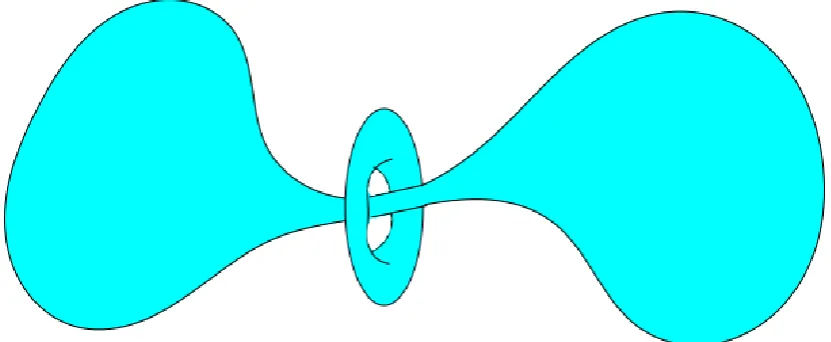
Angenent’s Doughnut Angenent [6] first proved the existence of a self-shrinking torus under the Mean Curvature Flow. In particular he shows that there exists an embedding of the 2-torus, X0 :T2 →R3 for which the corresponding solution to 1.6 is given byX(p, t) = 2p(1−t)X0(p), that is to say a torus that will shrink to the origin by dilations, and become singular at t = 1. This torus is commonly referred to in the literature as Angenent’s Doughnut and can be used to prove the existence of certain other kinds of singularities of MCF. For instance, if we consider a dumbbell shaped surface, consisting of a sufficiently thin cylindrical “neck” connecting two bells, which around its neck we can surround by a (dis-joint) Angenent’s doughnut as displayed in figure 2.1. Then under MCF the two surfaces remain disjoint until one of them reaches a singularity. Furthermore if the “bells” of the dumbbell are large enough, this implies that the neck must pinch off before the “bells” contract to a point, thus separating the two spheres from each other. This example is also often referred to as Grayson’s Dumbbell where the neck can be seen pinching off in figure 2.2.

(46)

[image:46.595.69.485.103.274.2]

Figure 2.1: Angenent’s Shrinking Doughnut

more formally we say that a Mean Curvature Flow Mt encounters a neckpinch

singularity at finite time T, as shown in figure 2.2, if there exists an open subset

Nt ⊂ Mt that evolves in time such that there exists a local diffeomorphism

be-tweenNtand _Sn−1×_R. Note that the neck may have infinite length. These neck regions of high curvature will be targeted for removal by the surgery procedure. We remark that similar neckpinch singularities occur during the Ricci Flow which is what makes a surgery programme for Ricci Flow also possible.

Cylindrical Estimate We now recount a convexity estimate for MCF of 2-convex hypersurfaces.

Theorem 2.12. Let Mt, t∈[0, T[ be a smooth solution of Mean Curvature Flow

with n ≥3 and initial data satisfying |A|2 _≤ _R−2 _{for some positive constant} _R_.

Then, for any η >0 there exists a constant Cη =Cη(n, α)>0 such that

|A|2₋ H2

n−1 ≤ηH 2₊_C

ηR−2

on Mt for any t∈[0, T[

When we deal with MCF with surgery, Huisken and Sinestrari work with a class of hypersurfaces C(R, α) (see 3.9) which is where the positive constant

R comes from. The proof of the the above theorem follows using the standard techniques we used in the proof of Theorem 2.10 for the mean convex case. The difference is we choose our functionGσ,η slightly differently by introducing a factor

before the H2 term, that is we define Gσ,η as follows Gσ,η =

|A|2 ₋ 1

n−1 +η

H2

(47)

2.4. THE 2-CONVEX CASE 47

(a) initial surface and step 1

(b) neck-pinch singularity in step 2 and 3

[image:47.595.118.530.247.567.2]

(c) step 4 and 5

A Survey of Convexity Estimates and Singularities for Mean Curvature Flow with Surgery