Chapter 1
An Introduction to Fractional Diffusion
B.I. Henry, T.A.M. Langlands and P. Straka
School of Mathematics and Statistics, University of New South Wales,
Sydney, NSW 2052 Australia [email protected]
The mathematical description of diffusion has a long history with many different formulations including phenomenological models based on con-servation of mass and constitutive laws; probabilistic models based on random walks and central limit theorems; microscopic stochastic mod-els based on Brownian motion and Langevin equations; and mesoscopic stochastic models based on master equations and Fokker-Planck equa-tions. A fundamental result common to the different approaches is that the mean square displacement of a diffusing particle scales linearly with time. However there have been numerous experimental measurements in which the mean square displacement of diffusing particles scales as a frac-tional order power law in time. In recent years a great deal of progress has been made in extending the different models for diffusion to incorpo-rate this fractional diffusion. The tools of fractional calculus have proven very useful in these developments, linking together fractional constitu-tive laws, continuous time random walks, fractional Langevin equations and fractional Brownian motions. These notes provide a tutorial style overview of standard and fractional diffusion processes.
1.1. Mathematical Models for Diffusion
1.1.1. Brownian Motion and the Langevin Equation
Having found motion in the particles of the pollen of all the living plants which I had examined, I was led next to inquire whether this property continued after the death of the plant, and for what length of time it was retained.
Robert Brown (1828)1
When microscopic particles are suspended in a fluid they appear to vi-brate around randomly. This phenomenon was investigated systematically by Robert Brown in 18271after he observed the behaviour in pollen grains
suspended in water and viewed under a microscope. Brown’s interest at the time was concerned with the mechanisms of fertilization in flowering plants. Brown noticed that the pollen grains were in a continual motion that could not be accounted for by currents in the fluid. One possibility favoured by other scientists at the time was that this motion was evidence of life itself, but Brown observed similar motion in pollen grains that had been dena-tured in alcohol and in other non-living material (including “molecules in the sand tubes, formed by lightning”1) .
The explanation for Brownian motion that is generally accepted among scientists today was first put forward by Einstein in 1905.2 The motion of
the suspended particle (which, for simplicity, was considered in one spatial direction) arises as a consequence of random buffeting from the thermal motions of the enormous numbers of molecules that comprise the fluid. This buffeting provides both the driving forces and the damping forces (the effective viscosity of the fluid) that are experienced by the suspended particle. The central result of Einstein’s theory is that in a given timet, the mean square displacementr(t) of a suspended particle in a fluid is given by
hr2(t)i= 2Dt (1.1)
where the angular brackets denote an ensemble average obtained by repeat-ing the experiment many times and the constant
D=
RT 6N πaη
=
kBT γ
. (1.2)
Here T is the temperature of the fluid, R = N kB is the universal gas constant,ais the radius of the suspended particle,η is the fluid viscosity, N is Avogadro’s number (the number of molecules in an amount of mass equal to the atomic weight in grams) and
γ= 6πηa (1.3)
is Stokes’ relation for the viscous drag coefficient. The results in Eqs. (1.1), (1.2) are known as the Einstein relations. In an interesting footnote to this literature, the Einstein relation in Eq. (1.2), was also derived independently by Sutherland.3
A very simple derivation (infinitely more simple4) of the Einstein
years later4based on Newton’s second law applied to a spherical particle in
a fluid. The mass times the acceleration is the sum of the random driving force and the frictional viscous force, both arising from the thermal motions of the molecules of the fluid:
md
2x
dt2 =F(t)−γ
dx
dt. (1.4)
The random driving force is assumed to have zero mean,hF(t)i= 0, and to be uncorrelated with position,hxF(t)i=hxihF(t)i= 0. Equation (1.4) can be simplified by multiplying byx(t), re-writing the left hand side as
mxd
2x
dt2 =m
d dt xdx dt −m dx dt 2 (1.5)
and then taking the ensemble average. This results in
m d dt xdx dt −m * dx dt 2+
=−γ
xdx dt
. (1.6)
A further simplification can be made using Boltzmann’s Principle of Equipartition of Energy5 which asserts that the average kinetic energy of
each particle in the fluid is proportional to the temperature of the fluid; in-dependent of the mass of the particle. The suspended particle being much larger in mass than the molecules of the fluid will have much smaller ve-locity according to this result. Applying this principle to the suspended particle we have
1 2m * dx dt 2+ =1
2kBT (1.7)
and Eq. (1.6) can be rearranged as dy dt +
γ my=
kBT
m (1.8) where y= xdx dt . (1.9)
Equation (1.8) is straightforward to integrate yielding
y =kBT γ
1−exp(−mγt). (1.10)
To proceed further we note that
y≡ xdx dt = 1 2 d dthx
2
so that
d dthx
2
i=2kBT γ
1−exp(−mγt).
For a Brownian particle that is large relative to the average separation between particles in the fluid, Langevin notes that mγ
≈108and so after
observational timest≫10−8 we have
d dthx
2
i ≈ 2kBT γ and hence
hx2i ∼
2k
BT γ
t= 2Dt (1.11)
in agreement with the Einstein relations in Eqs. (1.1), (1.2). In three spatial dimensions there are three kinetic degrees of freedom and the mean square displacement ishr2i ∼6Dt.
1.1.2. Random Walks and the Central Limit Theorem
The lesson of Lord Rayleigh’s solution is that in open country the most probable place to find a drunken man who is at all capable of keeping on his feet is somewhere near his starting point!
Karl Pearson (1905)6
The Brownian motion of the suspended particle in a fluid can also be modelled as a random walk, a term first introduced by Pearson in 19056
who sought the probability that a random walker would be at a certain distance from their starting point after a given number of random steps. The problem was solved shortly after by Lord Rayleigh.7 The idea of a random walk had been introduced earlier though by Bachelier in 1900 in his doctoral thesis (under the guidance of Poincar´e) entitledLa Theorie de la Speculation.8 In this thesis Bachelier developed a mathematical theory for
stock price movements as random walks, noting that ... the consideration of true prices permits the statement of the fundamental principle – The mathematical expectation of the speculator is zero.8
1.1.2.1. Random Walks and the Binomial Distribution
The probabilityPm,nthat the particle will be at positionx=m∆xat time t=n∆tis governed by the recurrence equation:
Pm,n= 1
2Pm−1,n−1+ 1
2Pm+1,n−1, (1.12)
withP0,0= 1. Note too that after any time kthe sum of the probabilities
must add up to unity and the largest possible excursion of the random walker afterntime steps is to position±n∆xso that
k
X
j=−k
Pj,k= 1 where k= 0,1,2, . . . n. (1.13)
The recurrence equation, Eq. (1.12) is a partial difference equation and although a solution could be sought using the method of separation of variables this generally results in complicated algebraic expressions.
An alternate method is to enumerate the number of possible paths in annstep walk from 0 tom. Without loss of generality this occurs through ksteps to the right andn−k=k−msteps to the left. Theksteps to the right can occur anywhere among thensteps. There are
C(n, k) =
n k
= n!
k!(n−k)!
ways of distributing theseksteps among thensteps. There are 2n possible paths in annstep walk so that the probability of annstep walk that starts at 0 and ends atmwithk steps to the right is given by
p(m, n) =C(n, k)
2n where k=
n+m
2 .
This simplifies to
p(m, n) = n!
2n n+m
2
! n−m
2
!. (1.14)
Note that we requiren+mandn−mto be even which is consistent with the recognition that it is not possible to get from the origin to an even (odd) lattice sitemin an odd (even) number of steps n.
The above result assumes an equal probability of steps to the left and right but it is easy to generalize with a probability r to step to the right and a probability 1−rto step to the left. The probability ofksteps to the right in annstep walk in this case is
P(k) =
n k
This is the probability mass function for the binomial distribution, i.e., if X is a random variable that follows the binomial distributionB(n, k) then P(k) =P rob(X=k). Note that in this biased random walk generalization we have
p(m, n) = n+m n!
2
! n−m
2
!r
n+m
2 (1−r)
n−m
2 . (1.16)
1.1.2.2. Random Walks and the Normal Distribution
Most of the results in this article are concerned with long time behaviours. In the case ofp(m, n) we consider n large and n > mbut m2/n
nonvan-ishing. It is worthwhile considering the behaviour of p(m, n) in this limit. Here we consider the simple case of the unbiased random walk, Eq. (1.14), but the analysis can readily be generalized.10 The mean number of steps to
the right ishki=n/2 and we consider the distribution for the fluctuations X =k− hki=m/2. We now have
p(m(X), n) = n!
(n2−X)!(n2 +X)!2n (1.17)
which can be expanded using the De Moivre-Stirling approximation9
n!≈√2πnnne−n (1.18)
to give
P(X, n) =
q 2
nπ
1−2X n
(n2−X+12) 1 + 2X n
(n2+X+12)
=
q 2
nπ
exp
(n
2 −X+ 1
2) ln(1− 2X
n ) + ( n
2 +X+ 1 2) ln(1 +
2X n )
.
The long time behaviour is now found after carrying out a series expansion of the log terms in powers of 2X
n . The result is
P(X, n)∼
r
2 nπe
−2X2 n =
r
2 nπe
−m2
2n. (1.19)
1.1.2.3. Random Walks in the Continuum Approximation
Further insights into the random walk description can be found by employ-ing a continuum approximation in the limit ∆x→0 and ∆t→0. In this approximation we first writeP(m, n) =P(x, t) and then re-write Eq. (1.12) as follows:
P(x, t) =1
2P(x−∆x, t−∆t) + 1
2P(x+ ∆x, t−∆t). (1.20)
Now expand the terms on the right hand side as Taylor series inx, t:
P(x±∆x, t−∆t)≈P(x, t)∓∆x∂P ∂x −∆t
∂P ∂t +
(∆x)2 2
∂2P ∂x2 +
(∆t)2 2
∂2P ∂t2
+∆t∆x∂
2P
∂x∂t+O((∆t)
3)
∓O((∆x)3).
If we substitute these expansions into Eq. (1.20) and retain only leading order terms in ∆tand ∆x, then after rearranging
∂P ∂t =D
∂2P
∂x2 (1.21)
where
D= lim
∆t→0,∆x→0
(∆x)2
2∆t (1.22)
is a constant with dimensions of m2s−1. The above partial differential
equation is known as the diffusion equation (see below).
The continuum approximation for the probability conservation law in Eq. (1.13) is
Z +∞ −∞
P(x, t)dx= 1 (1.23)
where the limits to infinity are consistent with taking the spacing between steps ∆x→0.
The fundamental Green’s solutionG(x, t) of the diffusion equation with initial conditionG(x,0) =δ(x) can readily be obtained using classical meth-ods. The Fourier transform of the diffusion equation yields
dG(q, t)ˆ
dt =−Dq
2G(q, t)ˆ
with solution
ˆ
where we have used the result that ˆG(q,0) = ˆδ(q) = 1. The inverse Fourier transform now results in
G(x, t) = 1 2π
Z +∞ −∞
e−Dq2t+iqxdq= 1 2πe
−x2
4Dt Z +∞
−∞
e−Dt(q− ix
2Dt)
2
dq
which simplifies to
G(x, t) = √ 1 4πDte
−x2
4Dt. (1.25)
The mean square displacement can be evaluated directly from
hx2i=
Z +∞ −∞
x2G(x, t)dx (1.26)
or indirectly from
hx2i= lim q→0−
d2
dq2G(q, t)ˆ (1.27)
yielding the familiar resulthx2i= 2Dt.
1.1.2.4. Central Limit Theorem
The fundamental solution, Eq. (1.25), is an example of the Gaussian normal distribution
P(X ∈dz) = √ 1 2πσ2exp
−(z−µ)
2
2σ2
(1.28)
for random variablesX with mean
µ=hXi (1.29)
and variance
σ2=hX2i − hXi2=hX2i −µ2. (1.30)
The Gaussian probability distribution, Eq. (1.25), can be derived indepen-dently for random walks by appealing to the Central Limit Theorem (CLT): The sum of N independent and identically distributed random variables with mean µ and variance σ2 is a Gaussian probability density function
with mean N µ and variance N σ2. In the case of random walks, each
step ∆x is a random variable with mean µ = h∆xi = 0 and variance σ2=h∆x2i − h∆xi2=h∆x2i.The sum ofN such random variables isxso
that from the CLT we have
P(x∈dz) = p 1
2πNh∆x2iexp
− z
2
2Nh∆x2i
But h∆x2i = 2Dh∆ti and N = t/∆t so that we recover Eq. (1.25) for
X =x.
This treatment of random walks using the CLT can be applied even if the step length ∆x varies between jumps, provided that the step lengths ∆x(t) are independent identically distributed random variables, i.e.,
h∆xi∆xji=δi,jh∆xii2.
In anN step walk with jumps at discrete timesti= (i−1)∆twe can define the average drift over timet=N∆t as
hx(t)i= N
X
i=1
h∆xii
and an average drift velocity as
v=hx(t)i ∆t . The variance of the random walk is
hx(t)2i − hx(t)i2= N
X
i=1
N
X
j=1
(h∆xi∆xji − h∆xiih∆xji).
Since the walks are uncorrelated this simplifies to
hx(t)2i − hx(t)i2=N h∆x2i − h∆xi2
=N σ2= 2Dt. (1.32)
Note that if the walk is biased then the drift velocity is non-zero and the probability density function is the solution of an advective-diffusion equa-tion (see below).
1.1.3. Fick’s Law and the Diffusion Equation
Equation (1.25) governing the probability of a random walker at positionx after timetis the probability distribution that should result if we measured the positions of a large number of particles in many separate experiments. However if the particles did not interact then we could perform measure-ments of their positions in the one experiment. The number of particles per unit volume at positionxand timetis the concentrationc(x, t). If there are N non-interacting walkers in total then they all have the same probability of being atxat timetand hence the concentrationc(x, t) =N P(x, t) also satisfies the diffusion equation
∂c ∂t =D
∂2c
We now consider a macroscopic derivation of the diffusion equation based on the conservation of matter and an empirical result known as Fick’s Law. The derivation is given in one spatial dimension for simplicity (this may describe diffusion in a three dimensional domain but with one-dimensional flow). In addition to the concentration c(x, t) other macro-scopic quantities of interest are the mean velocity u(x, t) of diffusing par-ticles, and the fluxq(x, t) which, in one spatial dimension, is the number of particles per unit time that pass through a test area perpendicular to the flow in the positivexdirection. The three macroscopic quantities are related through the equation
q(x, t) =c(x, t)u(x, t). (1.34)
Note that while the concentration is a scalar quantity both the mean ve-locity and the flux are vectors.
If no particles are added or removed from the system then, considering a small test volumeV of uniform cross-sectional area Aand extensionδx we have conservation of matter,
number of particles in volumeV at timet+δt
=
number of particles in volumeV at timet
+
net number of particles entering volume V betweentandt+δt
so that
c(x, t+δt)Aδx=c(x, t)Aδx+q(x, t)Aδt−q(x+δx, t)Aδt. (1.35)
Now divide byAδtδx and re-arrange terms then c(x, t+δt)−c(x, t)
δt =−
q(x+δx)−q(x, t)
δx (1.36)
and in the limitδt→0, δx→0, ∂c ∂t =−
∂q
∂x. (1.37)
The equation of conservation of matter (1.37) for flow in one spatial dimen-sion is also called thecontinuity equation.
Fick’s Law11 asserts that the net flow of diffusing particles is from
re-gions of high concentration to rere-gions of low concentration and the magni-tude of this flow is proportional to the concentration gradient. Thus
q(x, t) =−D∂c
∂x, (1.38)
is increasing in the xdirection (i.e., ∂x∂c > 0) then the flow of particles is in the negativexdirection. The constant of proportionality is the diffusion coefficient. If we combine the equation of conservation of matter, Eq. (1.37), with Fick’s Law, Eq. (1.38), then we obtain
∂c ∂t =
∂ ∂x
D∂c ∂x
=D∂
2c
∂x2 for constant D. (1.39)
One of the most significant aspects of Einstein’s results for Brownian motion is that the diffusivity can be related to macroscopic physical properties of the fluid and the particle, as in Eq. (1.2).
1.1.3.1. Generalized Diffusion Equations
The macroscopic diffusion equation is easy to generalize to higher dimen-sions and other co-ordinate systems. Examples are the diffusion equation in radially symmetric co-ordinates inddimensional space
∂c ∂t =
1 rd−1
∂ ∂r
rd−1D∂c ∂r
. (1.40)
Other generalizations of the macroscopic diffusion equation are possible by modifying Fick’s law. If the media is spatially heterogeneous then an ad-hoc generalization would be to replace the diffusion constant in Fick’s law with a space dependent function, ie.,D=D(x). Concentration dependent diffusivities and time dependent diffusivities have also been considered.
If the diffusing species are immersed in a fluid that is moving with velocityv(x, t) then this will produce anadvective flux
qA(x, t) =c(x, t)v(x, t). (1.41)
which, when combined with the Fickian flux, Eq. (1.38) and the continuity equation, Eq. (1.37), results in the advective-diffusion equation,
∂c ∂t =D
∂2c
∂x2 −
∂
∂x(v c). (1.42)
A possible generalization of the above equation for spatially inhomogeneous systems is then
∂c ∂t =
∂ ∂x
D(x)∂c ∂x
− ∂
∂x(v(x)c). (1.43)
is modelled by assuming that species move in the direction of a chemical gradient, thus
qC(x, t) =χc(x, t) ∂
∂xu(x, t), (1.44)
where u(x, t) is the concentration of the chemical species that is driving the chemotactic flux. This flux term is positive if the associated flow is from regions of low concentration to high concentration (chemoattractant, χ >0) and negative otherwise (chemorepellant,χ <0). The chemotactic diffusion equation in one dimension is
∂c ∂t =D
∂2c
∂x2−χ
∂ ∂x
c∂u ∂x
. (1.45)
1.1.4. Master Equations and the Fokker-Planck Equation
In his classic 1905 paper on Brownian motion, Einstein2derived the
diffu-sion equation from an integral equation conservation law or master equa-tion. The master equation describes the evolution of the probability density functionP(x, t) for a random walker taking jumps at discrete time inter-vals ∆tto be at positionxat timet. We letλ(∆x) denote the probability density function for a jump of length ∆xthen
P(x, t) =
Z +∞ −∞
λ(∆x)P(x−∆x, t−∆t)d∆x (1.46)
expresses the conservation law that the probability for a walker to be at x at time t is the probability that the walker was at position x−∆x at an earlier time t−∆t and then the walker jumped with step length ∆x. The integral sums over all possible starting points at the earlier time. The correspondence between the master equation and the diffusion equation (or a more general Fokker-Planck equation) can be found by considering continuum approximations in the limit ∆t→0 and ∆x→0, thus
P|(x,t−∆t)+ ∆t
∂P ∂t
(x,t−∆t)≈ Z +∞
−∞
λ(∆x) P|(x,t−∆t)−∆x
∂P ∂x
(x,t−∆t)
+ (∆x)
2
2 ∂2P
∂x2
(x,t−∆t) !
d∆x.
The integral over ∆xis simplified by noting that
Z +∞ −∞
Thus in the continuum limit the master equation yields the Fokker-Planck equation (also called the Kolmogorov forward equation)
∂P ∂t ≈
h∆x2i
2∆t ∂2P
∂x2 −
h∆xi ∆t
∂P
∂x, (1.47)
with drift velocity
v= lim
∆x→0,∆t→0
h∆xi
∆t , (1.48)
and diffusion coefficient
D= lim
∆x→0,∆t→0
h∆x2i − h∆xi2
2∆t =∆x→0lim,∆t→0
h∆x2i
2∆t +O
h∆xi2
∆t
(1.49)
so that
∂P ∂t ≈D
∂2P
∂x2 −v
∂P
∂x. (1.50)
1.1.4.1. Generalized Fokker-Planck Equation
If the step length probability density function is also dependent on position then the master equation generalizes to
P(x, t) =
Z +∞ −∞
λ(∆x, x−∆x)P(x−∆x, t−∆t)d∆x. (1.51)
In the continuum limit we proceed as above but with the additional expan-sion
λ(∆x, x−∆x)≈λ|(∆x,x)−∆x
∂λ ∂x
(∆x,x)
+∆x
2
2 ∂2λ
∂x2 (∆x,x)
, (1.52)
and
Z +∞ −∞
∆xnλ(∆x, x)d∆x=h∆xn(x)i,
which leads to the general Fokker-Planck equation
∂P ∂t =
∂2
∂x2(D(x)P(x, t))−
∂
∂x(v(x)P(x, t)), (1.53)
with drift
v(x) = lim
∆x→0,∆t→0
h∆x(x)i
∆t , (1.54)
and diffusivity
D(x) = lim
∆x→0,∆t→0
h∆x2(x)i − h∆x(x)i2
2∆t =∆x→0lim,∆t→0
h∆x2(x)i
The generalized Fokker-Planck equation, Eq. (1.53) is slightly different to the generalized Fickian equation, Eq. (1.43) (see further comments in Vlahoset al12and references therein).
1.1.5. The Chapman-Kolmogorov Equation and Markov
Processes
The sequence of jumps {Xt} in a random walk defines a stochastic pro-cess. A realization of this stochastic process defines a trajectory x(t). A stochastic process has the Markov property if at any time t the distribu-tion of all Xu, u > tonly depends on the value Xt and not on any value Xs, s < t. Letp(x, t) denote the probability density function forXtand let q(x, t|x′, t′) denote the conditional probability thatX
t lies in the interval x, x+dxgiven thatXt′ starts atx′. A first order Markov process has the
property that
q(x, t|x′′, t′′) =
Z
q(x, t|x′, t′)q(x′, t′|x′′, t′′)dx′. (1.55)
This equation, which was introduced by Bachelier in his PhD thesis,8 is
commonly referred to as the Chapman-Kolmogorov equation, in recogni-tion of the more general equarecogni-tion derived independently by Chapman and Kolmogorov for probability density functions in stochastic processes. We will refer to the special case as the Bachelier equation. Note that if we multiply the Bachelier equation byp(x′′, t′′) and integrate overx′′ then
Z
p(x′′, t′′)q(x, t|x′′, t′′)dx′′
=
Z
p(x′′, t′′)
Z
q(x, t|x′, t′)q(x′, t′|x′′, t′′)dx′
dx′′
=
Z Z
p(x′′, t′′)q(x′, t′|x′′, t′′)dx′′
q(x, t|x′, t′)dx′
so that
p(x′, t′) =
Z
p(x′′, t′′)q(x′, t′|x′′, t′′)dx′′
or equivalently
p(x, t) =
Z
p(x′, t′)q(x, t|x′, t′)dx′. (1.56)
Note that in the above we consider the times t > t′ > t′′ to be discrete
1.1.5.1. Wiener Process
It is easy to confirm by substitution that the conditional probability
q(x, t|x′, t′) = p 1
2π(t−t′)e −(2(x−xt−t′′)2)
, t > t′ (1.57)
is a solution of the Bachelier equation and
p(x, t) =√1 2πte
−x2
2t (1.58)
is a solution of Eq. (1.56) with this conditional probability. The corre-sponding Markov process is referred to as the Wiener process or Brownian motion. It is the limiting behaviour of a random walk in the limit where the time increment approaches zero. That this limit exists was proven by Norbert Wiener in 1923.13
The Brownian motion stochastic processBtsatisfies the following prop-erties:
(i)B0= 0 andBtis defined for timest≥0.
(ii) Realizations xB(t) of the process are continuous but nowhere differ-entiable. The graph of xB(t) versus t is a fractal with fractal dimension d= 3/2.
(iii) The increments Bt−Bt′ are normally distributed random variables
with mean 0 and variancet−t′ fort > t′.
(iv) The incrementsBt−Bt′ andBs−Bs′ are independent random variables
fort > t′≥s≥s′≥0.
1.1.5.2. Poisson Process
Another important Markov process is the Poisson point process. Here the spatial variable is replaced with a discrete variable labelling the occurrence of events (e.g., the numbers of encounters with injured animals on a road trip). The defining equations are
q(n, t|n′, t′) = (α(t−t
′))n−n′
(n−n′)! e −α(t−t′)
, t > t′ (1.59)
and
p(n, t) =(αt) n
n! e
−αt, (1.60)
andαtis the expected number of events in this interval. For example in an nstep random walk the expected number of steps to the right in time tis np= t
∆tpwherepis the probability to step to the right and ∆tis the time interval between steps. From the Poisson distribution the probability ofk steps to the right is
p(k, t) =( p
∆tt)k k! e
−(∆ptt). (1.61)
This can be reconciled with the Binomial distribution Eq. (1.15) by con-sidering the limitn→ ∞but npandk finite. Note that this requires that the probabilitypof a step to the right must be very small,p→0, and the Poisson distribution is thus the distribution law for rare events.
1.2. Fractional Diffusion
In the theory of Brownian motion the first concern has always been the calculation of the mean square displacement of the par-ticle, because this could be immediately observed.
George Uhlenbeck and Leonard Orntstein (1930)14
Central results in Einstein’s theory of Brownian motion are that the mean square displacement of the Brownian particle scales linearly with time and the probability density function for Brownian motion is the Gaussian nor-mal distribution. These characteristic signatures of standard diffusion are consistent across many different mathematical descriptions; random walks, central limit theorem, Langevin equation, master equation, diffusion equa-tion, Wiener processes. The results have also been verified in numerous ex-periments including Perrin’s measurements of mean square displacements15
to determine Avogadro’s number (the constant number of molecules in any mole of substance) thus consolidating the atomistic description of nature.
Despite the ubiquity of standard diffusion it is not universal. There have been numerous experimental measurements of fractional diffusion in which the mean square displacement scales as a fractional power law in time (see Table 1.1). The fractional diffusion is referred to as subdiffusion if the fractional power is less than unity and superdiffusion if the fractional power is greater than unity. Fractional diffusion has been the subject of several highly cited reviews,16–18and pedagogic lecture notes,12,19in recent
In the remainder of these notes we describe theoretical frameworks based around the physics of continuous time random walks and the mathematics of fractional calculus to model fractional diffusion. For a more complete de-scription the reader should again consult the review articles and references therein.
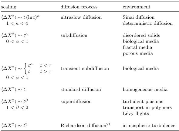
Table 1.1. Summary table of scaling laws for fractional diffusion
scaling diffusion process environment
h∆X2i ∼t(lnt)κ ultraslow diffusion Sinai diffusion 1< κ <4 deterministic diffusion
h∆X2i ∼tα subdiffusion disordered solids 0< α <1 biological media
fractal media porous media
h∆X2i ∼
tα t < τ
t t > τ transient subdiffusion biological media 0< α <1
h∆X2i ∼t standard diffusion homogeneous media
h∆X2i ∼tβ superdiffusion turbulent plasmas 1< β <2 transport in polymers
L´evy flights
h∆X2i ∼t3 Richardson diffusion21 atmospheric turbulence
1.2.1. Diffusion on Fractals
Experimental simulations and theoretical results have shown that diffusion on self-similar fractal lattices with fractal dimensiondf is anomalous sub-diffusion with scaling20
hr2i ∼tdw2 , d
w>2. (1.62)
The scaling exponentdw is referred to as the dimension of the walk. For standard random walks on Euclidean lattices ind= 2 the dimension of the walk is alsodw= 2. Equation (1.62) can be re-written as
hr2i ∼D(r)t (1.63)
provided that
D(r) =r2−dw. (1.64)
If we now reconsider the radially symmetric diffusion equation, Eq. (1.40), but replace the space dimension dwith the fractal dimension df and re-place the diffusion constant D with the spatially varying diffusion coeffi-cientD(r) then we arrive at the O’Shaugnessy Procaccia fractional diffusion equation22
∂c ∂t =
1 rdf−1
∂ ∂r
rdf−1r2−dw∂c
∂r
. (1.65)
1.2.2. Fractional Brownian Motion
One of the easiest ways to model anomalous subdiffusion is to replace the constant diffusivity with a time dependent diffusivityD(t) =αtα−1D. The
evolution equation for the concentration in this case is given by
∂c ∂t =αt
α−1D∂2c
∂x2. (1.66)
The solution is a Gaussian distribution
c(x, t) = √ 1
4πDtαexp
− x
2
4Dtα
. (1.67)
The probability density function for this stochastic process is non-Markovian due to the power law diffusivity. The mean square displacement is given by
hx2i= 2Dtα= 2Dt2H (1.68)
where H is the Hurst exponent. The fractional diffusion equation in Eq. (1.66) describes the probability density function for fractional Brow-nian motion.23 As an aside it is interesting to note that the power law
diffusivity may be expressed as a fractional derivative of a constant,
D(t) =0D1−t α(Γ(α)D), (1.69)
where 0D1−t α denotes a Riemann-Liouville derivative of order 1−α (see further details in the Appendix, Eq.(1.166)).
Starting with Mandelbrot and Van Ness24 there is a vast literature on
(i) Correlations
E(BH(t)BH(s)) = 1 2 |t|
2H+
|s|2H− |t−s|2H
,
(ii) Self similarity
BH(at)∼ |a|HBH(t),
(iii) Realizations xB(t) of the process are continuous but nowhere dif-ferentiable. The graph ofxB(t) versus t is a fractal with fractal dimensiond= 2−H.
Fractional Brownian motion can also be described by an evolution equa-tion of the form
x(t) =x0+0D−tαF(t). (1.70)
In this equation x(t) denotes the position of a random walker at time t given that it started atx0and F(t) is Gaussian white noise with
autocor-relationhF(t)F(s)i=δ(t−s). The evolution equation, Eq. (1.70), defines fractional Brownian motionx(t)−x0as a fractional integral (see Appendix
Eq.(1.158)), of order α, of white noise; and standard Brownian motion as an ordinary integral of white noise.
Fractional Brownian motion can also be derived from a microscopic fractional Langevin equation25,26
mdv dt =F
H(t)
−m
Z t 0
γ(t−t′)v(t′)dt′ (1.71)
where FH(t) denotes coloured noise with vanishing mean and correla-tion related to the dissipative memory kernelγ(t) through a fluctuation-dissipation theorem25
hFH(t)FH(0)i=mkbT γ(t). (1.72)
In the particular caseγ(t) = Dα mkBTt
−α the fractional Langevin equation
mdv dt =F
H(t)
−m0Dαt−1v(t) (1.73)
describes subdiffusion for 0< α <1. The probability density function for trajectories that satisfy the fractional Langevin equation has been shown to be23,27 the fractional Brownian motion diffusion equation, Eq. (1.66).
is referred to as temporal memory and it is related to the non-Markovian property. The mathematics of fractional calculus has a long history dating back to Leibniz (1965) but it has only been in recent decades that frac-tional calculus has permeated mainstream physics literature. The recent interest in fractional calculus in physics is largely due to the relevance of fractional calculus for the physical problem of anomalous diffusion. The keen student would be well advised to acquaint themselves with some of the general mathematical results on fractional calculus in the Appendix before proceeding with the remainder of these notes on fractional diffusion.
1.2.3. Continuous Time Random Walks and Power Laws
It was the man from Ironbark who struck the Sydney town, he wandered over street and park, he wandered up and down. He loitered here, he loitered there ...
A.B “Banjo” Paterson
The Bulletin, 17 December 1892.
1.2.3.1. CTRW Master Equations
In the standard random walk the step length is a fixed distance ∆xand the steps occur at discrete times separated by a fixed time interval ∆t. A more general random walk can be obtained by choosing a waiting time from a waiting time probability density before each step and then choosing the step length from a step length probability density. These more general walks are Continuous Time Random Walks (CTRWs) . They were introduced by Montroll and Weiss in 196528(see also Scher and Lax29 and Montroll and
Shlesinger30).
The fundamental quantity to calculate is the conditional probability densityp(x, t|x0, t0) that a walker starting from positionx0 at time t= 0, is atpositionxat timet. The conditional probability densityqn(x, t|x0, t0)
that afternsteps a walker starting atx0 at timet= 0 arrives atposition
xat timetsatisfies the recursion relation
qn+1(x, t|x0,0) = Z +∞
−∞ Z t
0
Ψ(x−x′, t−t′)qn(x′, t′|x0,0)dt′
dx′ (1.74) where Ψ(x−x′, t−t′) is the probability density that in a single step a
random walker steps a distance x−x′ after waiting a time t−t′. This
arrival densityqsatisfies the initial condition
and the normalization
Z +∞ −∞
Z ∞ 0
q0(x′, t′|x0,0)dt′dx′= 1.
The conditional probability density that a walker arrives at positionx at timet after any number of steps is given by
q(x, t|x0,0) = ∞ X
n=0
qn(x, t|x0,0). (1.75)
After summing over n, and using the initial condition, in the recursion equation, Eq. (1.74), we can write29
q(x, t|x0,0) = Z +∞
−∞ Z t
0
Ψ(x′, t′)q(x−x′, t−t′|x0,0)dt′dx′+δ(t)δx,x0.
(1.76) In the theory of CTRWs it is assumed that waiting times are indepen-dent and iindepen-dentically distributed random variables with densityψ(t), t >0 and step lengths are independent and identically distributed random vari-ables with densityλ(x), x∈R. It is further assumed that the waiting times
and step lengths are independent of each other so that
Ψ(x−x′, t−t′) =λ(x−x′)ψ(t−t′). (1.77)
It follows from the normalization of the probability density functions that
ψ(t) =
Z +∞ −∞
Ψ(x′, t)dx′ (1.78)
and
λ(x) =
Z ∞ 0
Ψ(x, t′)dt′. (1.79)
It is also useful to define the survival probability
Φ(t) = 1−
Z t 0
ψ(t′)dt′=
Z ∞
t
ψ(t′)dt′ (1.80)
which is the probability that the walker does not step during time interval t(i.e., the waiting time is greater than t).
The conditional probability density that a walker starting from the ori-gin at time zero is at positionxat timetis now given by28
p(x, t|x0,0) = Z t
0
The right hand side considers all walkers that arrived at x at an earlier timet′ and thereafter did not step.
The results for the conditional probability densities in Eq. (1.76) and Eq. (1.81) can be combined to yield the fundamental master equation for CTRWs,
p(x, t|x0,0) = Φ(t)δx,x0+
Z t 0
ψ(t−t′)
Z +∞ −∞
λ(x−x′)p(x′, t′|x0,0)dx′dt′.
(1.82) The master equation can be justified using temporal Laplace transforms. The Laplace transform of Eq. (1.76) yields
ˆ
q(x, u|x0,0) = Z +∞
−∞
ˆ
Ψ(x′, u)ˆq(x−x′, u|x0,0)dx′+δx,x0.
The Laplace transform of Eq. (1.81) now yields
ˆ
p(x, u|x0,0) = ˆq(x, u|x0,0) ˆΦ(u)
=
Z +∞ −∞
ˆ
Ψ(x′, u) ˆΦ(u)ˆq(x−x′, u|x0,0)dx′+ ˆΦ(u)δx,x0
=
Z +∞ −∞
ˆ
Ψ(x′, u)ˆp(x−x′, u|x0,0)dx′+ ˆΦ(u)δx,x0.
The master equation, Eq. (1.82), is the inverse Laplace transform of the above equation. The master equation can also be justified using probability arguments. The first term represents the persistence of the walker at the initial position and the second term considers walkers that were at other positionsx′ at timet′ but then stepped toxat timetafter waiting a time
t−t′.
In the original formulation of the master equation the steps were as-sumed to take place on a discrete lattice, so that
p(x, t|x0,0) = Φ(t)δx,x0+
X
x′ Z t
0
ψ(t−t′)λ(x−x′)p(x′, t′|x0,0)dt′. (1.83)
The CTRW can also be described using a generalized (gain-loss) master equation of the form30
dP(x, t)
dt =
Z t 0
X
x′
(K(x, x′;t−t′)P(x′, t′)−K(x′, x;t−t′)P(x, t′))dt′.
transition fromxtox′ during timet−t′. The CTRW master equation can
be shown to be equivalent to the generalized master equation if30
K(x, x′;t−t′) =λ(x−x′)φ(t−t′) (1.85)
and
ˆ
φ(u) = uψ(u)ˆ
1−ψ(u)ˆ . (1.86)
It is straightforward to extend the CTRW master equation by consid-ering walkers starting from different starting points. The master equation for the expected concentration of walkers at positionxandtis then31
n(x, t) = Φ(t)n(x,0) +
Z +∞ −∞
Z t 0
n(x′, t′)ψ(t−t′)λ(x−x′)dt′dx′. (1.87)
We now consider different choices for the densities ψ(t) and λ(x) which result in different (possibly fractional) diffusion equations. The approach is as follows; decouple the convolution integrals in the master equation, Eq. (1.87), use a Fourier transform in space and a Laplace transform in time; consider asymptotic expansions of the transformed equation for small val-ues of the Fourier and Laplace variables; carry out inverse Fourier-Laplace transforms using fractional order differential operators (if needed). Some general results on fractional order derivatives are provided in the appendix. Here we introduce the operators as needed.
1.2.3.2. Exponential Waiting Times and Standard Diffusion
The Fourier-Laplace transform of the CTRW master equation yields
ˆ
ˆn(q, u) = ˆΦ(u)ˆn(q,0) + ˆψ(u)ˆλ(q)ˆˆn(q, u) (1.88)
whereqis the Fourier variable anduis the Laplace variable.
The Laplace transform of the survival probability can be written as
ˆ
Φ(u) = 1 u−
ˆ ψ(u)
u . (1.89)
To proceed further we assume asymptotic properties for the step length density and the waiting time density. To begin with we assume that the step length density has the asymptotic expansion
ˆ
λ(q)∼1−q
2σ2
2 +O(q
where
σ2=
Z
r2λ(r)dr, (1.91)
is finite. This is a general expansion for any even functionλ(x) = λ(−x) with a finite variance σ2. An example of such a density is the Gaussian
density
λ(x) = √ 1 2πσ2exp
−x
2
2σ2
. (1.92)
The Fourier-Laplace CTRW master equation can now be written as
uˆˆn(q, u) = (1−ψ(u))ˆˆ n(q,0) +uψ(u)ˆ
1−q
2σ2
2
ˆ
ˆn(q, u) (1.93)
Now consider a waiting time density with a finite meanτ then ˆ
ψ(u) = 1−τ u+O(u2). (1.94)
An example of such a density is the exponential density
ψ(t) = 1 τexp
−τt
. (1.95)
It is easy to verify the (memoryless) Markov property that the probability of waiting a time T > t+sconditioned on having waited a time T > sis equivalent to the probability of waiting a timeT > tat the outset:
P(T > t) =
Z ∞
t 1 τexp
−t
′
τ
dt′=e−τt
so that
P(T > t+s|T > s) = P(T > t+s) P(T > s) =e
−t
τ =P(T > t).
Using the exponential waiting time density we now have, to leading order,
uˆˆn(q, u) =τ uˆn(q,0) + (u−τ u2)
1−q
2σ2
2
ˆ
ˆn(q, u) (1.96)
which simplifies to
uˆˆn(q, u)−n(q,ˆ 0) =−σ
2q2
2τ ˆn(q, u). (1.97) The inverse Fourier and Laplace transforms now yield the standard diffusion equation
∂n ∂t =D
∂2n
where
D=σ
2
2τ. (1.99)
1.2.3.3. Power Law Waiting Times and Fractional Subdiffusion
The Markovian property of the exponential waiting time density contrasts with that of a Pareto waiting time density
ψ(t) = ατ α
t1+α t∈[τ,∞], 0< α <1. (1.100)
The cummulative distribution is a power law, 1− τt
α
. Three properties of note are; (i) the mean waiting time is infinite, (ii) the probability of waiting a time T > t+s, conditioned on having waited a time T > s, is greater than the probability of waiting a timeT > tat the outset (the waiting time density has a temporal memory ) and (iii) the waiting time density is scale invariant,ψ(γt) =γ−(1+α)ψ(t).
The asymptotic Laplace transform for the Pareto density is given by a Tauberian (Abelian) theorem as (see, e.g., Berkowitzet al32)
ˆ
ψ(u)∼1−Γ(1−α)ταuα. (1.101)
Again we assume that the step length density is an even function with finite variance and we substitute the above expansion into the Fourier-Laplace master equation, Eq. (1.93), retaining only leading order terms. This results in
uˆˆn(q, u)−n(q,ˆ 0) =− q
2σ2
2ταΓ(1−α)u
1−αˆˆn(q, u), (1.102)
and after carrying out the inverse Fourier-Laplace transform
∂n(x, t) ∂t =DL
−1
u1−α∂
2n(x, u)ˆ
∂x2
(1.103)
where
D= σ
2
2ταΓ(1−α). (1.104)
This can be simplified further by using a standard result in fractional cal-culus33 (see Appendix, Eq.(1.167)),
u1−α∂2n(x, u)ˆ
∂x2 =L 0D 1−α t n(x, t)
+
0D−tα
∂2n(x, t)
∂x2
t=0
In this equation0Dt1−αdenotes a Riemann-Liouville fractional derivative of orderαand 0D−tα denotes a fractional integral of orderα. The fractional integral on the far right hand side of Eq. (1.105) can be shown to be zero under fairly general conditions34 so that using Eq. (1.105) in Eq. (1.103)
we obtain the celebrated fractional subdiffusion equation ∂n(x, t)
∂t =D
0D1−t α
∂2n(x, t)
∂x2
. (1.106)
This equation can be obtained phenomenologically by combining the con-tinuity equation
∂n ∂t =−
∂q ∂x with an ad-hoc fractional Fick’s law
q(x, t) =−D
0D1−t α
∂n(x, t) ∂x
.
The fractional integral in this expression provides a weighted average of the concentration gradient over the prior history.
The Green’s solution for the subdiffusion equation can be written in closed form using Fox H functions17 (see Table 1.2). The special caseα=
1/2 is more amenable to analysis since the solution in this case can be written in terms of Meijer G-functions
G(x, t) =p 1 8πDt12
G30,,03
x2
16Dt21
0,1
4, 1 2
(1.107)
that are included as special functions in packages such as Maple and Math-ematica.
review article by Metzler and Klafter17 contains a useful summary of Fox
H function properties including a computable alternating series for their evaluation.
We now consider the mean square displacement
hx2(t)i=
Z ∞ −∞
x2G(x, t)dx (1.108)
which can be evaluated using the Fourier-Laplace representation
hx2(t)i=L−1
lim q→0−
d2
dq2
ˆ ˆ G(q, u)
. (1.109)
After rearranging Eq. (1.102) and using the result that ˆG(q,0) = 1 we have
ˆ ˆ
G(q, u) = 1
u+q2Du1−α (1.110)
and then using Eq. (1.109)
hx2(t)i=L−1 2Dαu−1−α= 2D Γ(1 +α)t
α. (1.111)
1.2.3.4. Subordinated Diffusion
The asymptotic subdiffusion that arises from a CTRW with power law wait-ing times can be considered as a subordinated Brownian motion stochastic process. IfB(t) denotes a Brownian motion stochastic process then a sub-ordinated Brownian motion stochastic process B(E(t)) can be generated from a non-decreasing stochastic processE(t) with values in [0,∞) which is independent of B(t) and which starts at E(0) = 0. Meerschaert and Scheffler,36 have shown that there is a one-to-one correspondence between CTRWs with radially symmetric jumps of finite variance, and processes of the form B(E(t)), where E(t) is the generalized inverse of a strictly increasing L´evy processS(t) on [0,∞).
In particular it is a straightforward exercise to show that ifn(x, t) is the Green’s solution of the time fractional subdiffusion equation,
∂n ∂t =0D
1−α t
∂2n
∂x2
then
n(x, t) =
Z ∞ 0
wheren⋆(x, τ) is the Green’s solution of the standard diffusion equation
∂n ∂τ =
∂2n
∂x2
andT(τ, t) is defined through the Laplace transform, with respect tot,17
ˆ
T(τ, u) =uα−1e−τ uα. (1.113)
The densityT(τ, t) is related to the one-sided L´evyα-stable densityℓα(z) through37
T(τ, t) = t ατα+1α
ℓα
t
τα1
. (1.114)
Equation (1.112) defines a subordination process for n(x, t) in terms of the operational time τ and the physical time t. The operational time is essentially the number of steps in the walk. In the standard random walk the number of steps is proportional to the physical time but in the CTRW with infinite mean waiting times the number of steps is a random variable. The solution of the time fractional diffusion equation at physical timetis a weighted average over the operational time of the solution of the standard diffusion equation.
1.2.3.5. L´evy Flights and Fractional Superdiffusion
We now consider CTRWs with an exponential (Markovian) waiting time density but a L´evy step length density with power law asymptotics
λ(x)∼Aσα α|x|
−1−α, 1< α <2. (1.115)
The L´evy step length density enables walks on all spatial scales.
Our starting point is the Fourier-Laplace transformed master equation, Eq. (1.88), combined with the Laplace transform of the survival probability, Eq. (1.89), i.e.,
uˆˆn(q, u) = (1−ψ(u))ˆˆ n(q,0) +uψ(u) ˆˆ λ(q)ˆˆn(q, u). (1.116)
The exponential waiting time density has a finite mean τ so that ˆψ(u)∼ 1−τ uand then
uˆˆn(q, u) =τ uˆn(q,0) + u−τ u2ˆ
λ(q)ˆˆn(q, u). (1.117)
The Fourier transform of the L´evy step length density is given by17
ˆ
The L´evy density can be expressed in terms of Fox H functions38 through
the inverse Fourier transform (see Appendix, Eq.(1.190). If we substitute Eq. (1.118) into Eq. (1.117) and retain leading order terms then we obtain
uˆˆn(q, u)−uˆn(q,0) =−σ α|q|α
τ ˆˆn(q, u), (1.119)
and then after inversion of the Laplace transform
∂n(q, t)ˆ ∂t =−
σα|q|α
τ n(q, t).ˆ (1.120)
It remains to invert the Fourier transform and this can be done using another standard result of fractional calculus
F∇α|x|n(x, t)
=−|q|αˆn(q, t) (1.121)
where∇µ|x|is the Riesz fractional derivative (see Appendix, Eq.(1.173)) and
F denotes the Fourier transform operator. The evolution equation for the probability density function is now given by
∂n ∂t =D∇
α
|x|n (1.122)
with the diffusion coefficient
D=σ α
τ . (1.123)
The solution, which can be expressed in terms of Fox H functions (see Table 2), has the asymptotic behaviour17
n(x, t)∼ σ αt
τ|x|1+α, 1< α <2. (1.124)
The mean square displacement diverges in this model, i.e., hx2(t)i → ∞.
This is an unphysical result but it is partly ameliorated by a non-divergent pseudo mean square displacement,
h[x2(t)]i ∼tα2, (1.125)
which can be inferred from the finite fractional moment scaling17
h|x|δi ∼tαδ, 0< δ < α <2. (1.126)
1.2.4. Simulating Random Walks for Fractional Diffusion In this section we describe Monte Carlo methods to simulate random walk trajectories (and thus generate probability density functions) for standard diffusion, fractional Brownian motion, subdiffusion, and superdiffusion. Al-gebraic expressions for the probability density functions are summarized in Table 1.2.
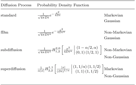
Table 1.2. Probability density functions for standard and fractional diffu-sion equations.
Diffusion Process Probability Density Function
standard √ 1
4πDte
−4xDt2 Markovian
Gaussian
fBm √ 1
4πDtαe
− x2
4Dtα Non-Markovian
Gaussian
subdiffusion √ 1 4πDtαH
2,0 1,2 »
x2
4Dtα
˛ ˛ ˛ ˛
(1−α/2, α) (0,1) (1/2,1)
–
Non-Markovian
Non-Gaussian
superdiffusion α1|x|H21,,21
» |x| (Dt)1/α
˛ ˛ ˛ ˛
(1,1/α) (1,1/2) (1,1) (1,1/2)
–
Markovian
Non-Gaussian
The general procedure for simulating a single trajectory is as follows:
(1) Set the starting position of the particle,x, and jump-time,t, to zero. (2) Generate a random waiting-time,δt, and jump-length,δx, from
appro-priate waiting-time and jump-length densities, ψ(t) and λ(x) respec-tively.
(3) Update the position of the particlex(t+δt) =x(t) +δx.
(4) Update the jump-time t = t+δt of the particle. For non-constant waiting-times (e.g. subdiffusion) both the position of the particle and its jump-time need to be stored.
(5) Repeat steps 1 to 4 until the new jump-time reaches or exceeds the required simulation run-time.
of random walk simulations.
1.2.4.1. Generation of waiting-times
In the subdiffusive case we take the waiting-time density as the (shifted) Pareto law39
ψ(t) = α/τ
(1 +t/τ)1+α. (1.127)
The parametersαandτ are the anomalous exponent and the characteristic time respectively. This probability density function has the asymptotic scaling
ψ(t)∼ατ
t τ
−1−α
(1.128)
for long times. A random waiting-time that satisfies the waiting-time den-sity, Eq. (1.127) can be generated from a uniform distribution ρ(r)dr = 1dr, r∈[0,1] as follows:
ρ(r)dr=ρ(r(t))dr
dtdt=ψ(t)dt (1.129)
butρ(r(t)) = 1 so that
dr
dt =ψ(t). (1.130)
The solution of Eq. (1.130), using Eq. (1.127), and the initial condition r(0) = 0 is given by
r(t) = 1−
1 + t τ
−γ
. (1.131)
We can now invert this equation to find the random waiting timet=δtin terms of the random numberr. This yields
δt=τ(1−r)−α1 −1
(1.132)
wherer∈(0,1) is a uniform random number.
For the non-subdiffusive cases we take for simplicity a constant waiting-time ofδt=τ between jumps. The density for this case is simply
ψ(t) =δ(t−τ) (1.133)
though the exponential density
ψ(t) = 1 τe
−t
could also be used. In this latter case the generated random waiting-time is given by
δt=−τln(1−r). (1.135)
1.2.4.2. Generation of jump-lengths
In the case of superdiffusion we generate a jump-length from the L´evy α-stable probability density using the transformation method described in:40,41
δx=σ
−lnucosφ cos ((1−α)φ)
1−1
α sin (αφ)
cosφ (1.136)
where φ=π(v−1/2),σ is jump-length scale parameter, andu, v∈(0,1) are two independent uniform random numbers.
For simplicity, the jumps in the non-superdiffusive cases are taken to the nearest-neighbour grid points only. For the standard diffusion and subdiffusive cases the particle, after waiting, has to jump either to the left or right a distance of ∆x. The jump-length, for these cases, is generated from
δx=
∆x, 0≤r < 12
−∆x, 12 ≤r <1
(1.137)
wherer∈(0,1) is uniform random number. The jump density in this case is
λ(x) =1
2δ(x−∆x) + 1
2δ(x+ ∆x). (1.138)
In the fractional Brownian case the particle may jump to the left or right or not jump at all. In this case Eq. (1.137) is modified to (where 0< α <1)
δx=
∆x, 0≤r < αnα−1
−∆x, αnα−1≤r <2αnα−1
0, 2αnα−1≤r <1
(1.139)
1.2.4.3. Calculation of the Mean-Squared Displacement
To calculate the mean-squared displacement for the non-superdiffusive cases we simply evaluate the ensemble average of the particles position, x(t), at each time-steptn=nτ. For simulations with a non-constant waiting time, this requires a bit of book-keeping as the particles do not necessarily jump at these times. However the position of the particle for a particular trajectory can be found from the stored jump-times noting the particles wait at their current location until the next jump-time. The mean-squared displacement is estimated using
x2(tn)≃ 1 M
M
X
j
[x(tn)]2 (1.140)
where M is the number of trajectories averaged. This can be compared with the algebraic expressions for the mean square displacements for subd-iffusion, Eq. (1.111), and standard diffusion (γ= 1) once the constantDis estimated. In the case of fractional Brownian motion, we can also compare with Eq. (1.111) but with denominator set to unity.
In the case of superdiffusion, where the mean-squared displacement di-verges, we have computed the ensemble average
D
|x|δ(tn)
E
≃ M1 M
X
j
[x(tn)]δ 0< δ < α (1.141)
to compare with17
D
|x|δ(t)E= 2 α(Dt)
δ/α Γ (−δ/α) Γ (1 +δ)
Γ (−δ/2) Γ (1 +δ/2). (1.142)
1.2.4.4. Probability Density Functions
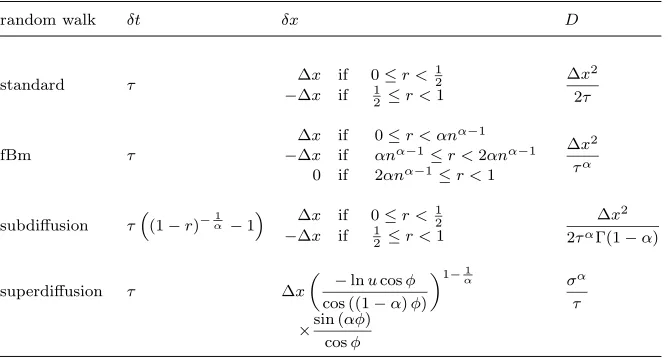
The waiting-times, δt, and step-lengths, δx, for simulating standard and fractional diffusion processes are listed in Table 1.3. The diffusion constants are also listed for the purposes of comparisons with the algebraic formulae in Table 1.2.
Table 1.3. Waiting times, step lengths and diffusion constants for simulating fractional diffusion random walks.
random walk δt δx D
standard τ ∆x if 0≤r <
1 2 −∆x if 12 ≤r <1
∆x2 2τ
fBm τ
∆x if 0≤r < αnα−1 −∆x if αnα−1≤r <2αnα−1
0 if 2αnα−1≤r <1
∆x2
τα
subdiffusion τ“(1−r)−α1 −1
” ∆x if 0≤r <1 2 −∆x if 12 ≤r <1
∆x2 2ταΓ(1−α)
superdiffusion τ ∆x
„
−lnucosφ cos ((1−α)φ)
«1−1α
σα τ
×sin (αφ) cosφ
In the table,r, u, v∈(0,1) are independent random numbers andφ=π(v−1/2),n=t/τ.
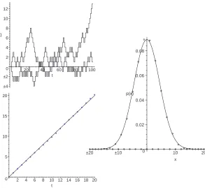
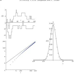
densities shown in these notes. In the fractional Brownian motion and sub-diffusion we took α= 1/2. For the superdiffusive case we used α = 3/2 and calculated the average Eq. (1.141) using δ= 3/4 = α/2. The results of the simulations are compared with algebraic results in Figs. 1.1–1.4. Note thelog−logscales in the mean-squared displacement plots. The data values correspond to logarithms of the numbers shown on the axes. In each case the results of the simulations (open circles) agree with the theoretical results (solid lines).
1.2.5. Fractional Fokker-Planck Equations
In the CTRWs described above we considered unbiased walks i.e., there was an equal probability to step left or right in a given step. It is possible to generalize the analysis to permit a bias, for example the step length density could be chosen to be a function of position to model the effects of CTRWs in a space varying force field. The biased CTRWs lead to fractional Fokker-Planck equations. In these notes we summarize key results that have been obtained and refer the reader to the original journal articles for details.
–4 –2 0 2 4 6 8 10 12
x(t)
20 40 60 80 100 t
0 0.02 0.04 0.06 0.08
p(x)
–20 –10 10 20
x
0 5 10 15 20
[image:35.612.149.442.207.476.2]2 4 6 8 10 12 14 16 18 20 t
Fig. 1.1. Sample trajectories (top left), probability density function (right) and mean-squared displacement (lower left) for standard diffusion.
two fractional Fokker-Planck equations that have been considered are ∂n(x, t)
∂t = 0D
1−α
t D∇2n(x, t)− 0D1−t α∇
1
ηf(x, t)n(x, t)
(1.143)
and ∂n(x, t)
∂t = 0D
1−α
t D∇2n(x, t)− ∇
1
ηf(x, t)0D
1−α
t ∇n(x, t)
(1.144)
where D is the diffusion coefficient for subdiffusion, Eq. (1.104), and the coefficentsD andη are related through a generalized Einstein relation
D= kBT
mη . (1.145)
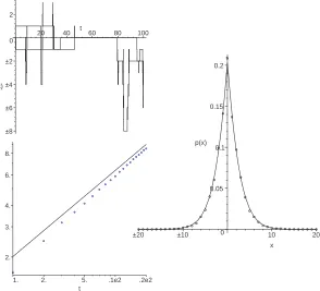
–4 –2 0 2 4
x(t)
20 40 t 60 80 100
0.02 0.04 0.06 0.08 0.1 0.12 0.14
p(x)
–20 –10 10 20
x
1. 2. 4. 7. .1e2 .2e2
[image:36.612.137.446.172.478.2]5. .1e2 .5e2 .1e3 t
Fig. 1.2. Sample trajectories (top left), probability density function (right) and log-log mean-squared displacement (lower left) for fractional Brownian motion withα= 1/2.
Eq. (1.143) has been derived from biased CTRWs42and in the case of
sub-diffusion in a space independent external force field f = f(t) the second fractional Fokker-Planck equation Eq. (1.144) has been derived from a gen-eralized master equation formulation of CTRWs.43
Given that both equations are equivalent in the case of time independent force fields this suggests that the second formulation might be preferred for generalizing to f = f(x, t). Another argument in favour of this is that temporal variations in the external force field occur in physical time which is different to the operational time for subdiffusion whereas the first formulation produces a subordination over the same operational time scale. However if the force field is generated internally (e.g., by ionic concentration gradients or chemotaxis) then this subordination may be appropriate.
–8 –6 –4 –2 0 2
x(t)
20 40 t 60 80 100
0 0.05 0.1 0.15
0.2
p(x)
–20 –10 10 20
x 2.
3. 4. 6. 8.
[image:37.612.150.444.210.477.2]1. 2. 5. .1e2 .2e2 t
Fig. 1.3. Sample trajectories (top left), probability density function (right) and log-log mean-squared displacement (lower left) for fractional subdiffusion withα= 1/2.
fractional diffusion in an external (or internal) time and space varying force field is still an open problem.
1.2.6. Fractional Reaction-Diffusion Equations
The CTRW formalism can also be extended to accommodate source or sink terms arising from reactions. These generalized CTRWs lead to fractional reaction-diffusion equations. Again, in these notes we simply summarize key results and refer the reader to the original journal articles for details.
In early CTRW formulations of fractional reaction-diffusion44 a time
fractional derivative was applied to the spatial diffusion term but not the reaction terms. However in other studies it was suggested that the time fractional derivative should operate equally on both terms.39,45 This second
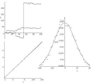
reac-0 50 100 150 200
x(t)
20 40 60 80 100 t
0.005 0.01 0.015 0.02 0.025 0.03 0.035 0.04
p(x)
–20 –10 0 10 20
x 2.
3. 4.
[image:38.612.147.445.204.478.2]1. 2. 5. .1e2 .2e2 t
Fig. 1.4. Sample trajectories (top left), probability density function (right) and log-log pseudo mean-squared displacement withδ= 3/4 (lower left) for fractional superdiffusion withα= 3/2.
tions and diffusions are affected by the same operational time scales. More recently, at least in the case of linear reaction dynamics, it was shown31,46
that neither approach properly describes subdiffusion with prescribed lin-ear reaction kinetics. In the particular case where the reaction dynamics models exponential growth (+k) or decay (−k) during the CTRW waiting time intervals the CTRW master equation yields the balance equation31
n(x, t) = Φ(t)e±ktn(x,0)+Z
∞
−∞ Z t
0
n(x′, t′)e±k(t−t′)
ψ(t−t′)λ(x−x′)dt′dx′
(1.146) and the governing fractional reaction diffusion equation is given by31
∂n ∂t =D e
±kt
0Dt1−α
e∓kt∂
2n
∂x2
The above formalism has also been extended to multispecies subdiffusion with linear reaction kinetics.47 Although some progress has been made in
extending CTRWs to include nonlinear reaction kinetics48 the derivation
of general nonlinear fractional reaction diffusion equations is still an open problem. A possible generalization of the balance equation, Eq.(1.146), for nonlinear reactions is to replace the linear evolution operatore±kt in this equation with a nonlinear evolution operator.
1.2.7. Fractional Diffusion Based Models
In addition to the fractional diffusion equations derived from CTRWs there are numerous other fractional diffusion equations that have been studied as models for physical, social or economic systems, with varying levels of justification. Examples include:
Space-time fractional Fokker-Planck equation17
∂w ∂t =D
1−α t
∂
∂x V′(x)
η +K∇|x|µ
w. (1.148)
Space-time fractional diffusion model for plasmas49
DβtP =χ∇|x|αP. (1.149)
Fractional Black-Scholes model for option prices50
rV(x, t) = ∂V(x, t)
∂t +
r+σαsec(απ 2 )
∂V
∂x −σ
αsec(απ 2 )D
α
xV. (1.150)
Fractional cable equation for nerve cells51
rmcm∂V ∂t =
drm 4rL(γ)D
1−γ t
∂2V ∂x2
− Dt1−κ(V −rmie). (1.151)
1.2.8. Power Laws and Fractional Diffusion
An average individual who seeks a friend twice his height would fail. On the other hand, one who has an average income will have no trouble in discovering a richer person with twice his income, and that richer person may, with a little diligence, locate a third party with twice his income, etc.
Elliot Montroll and Michael Shlesinger (1984)30
a first general remark, power laws f(x) are scale invariant functions, i.e., f(λx) =λαf(x) for some exponentα and all scale factors λ. Power law scaling is a characteristic feature of fractals, and power law distributions have been found to characterize numerous real world data sets52 in which
the complexity might be expected to extend over a large range of spatial or temporal scales.
A possible mechanism that has been suggested for power law waiting time densities in CTRWs53is that the random walker moves in an
environ-ment with an exponential distribution of trap binding energies
ρ(E) = 1 E0e
−E
E0 (1.152)
with thermally activated trapping times
τ =ekB TE . (1.153)
The waiting time density follows as
ψ(τ)dτ =ρ(E)dE dτ dτ
= 1
E0
e−EE0
kBT τ
dτ
= 1
E0
τ−kTE0
kBT τ
dτ
=
k
BT E0
τ−kTE0−1dτ,
so that
ψ(t) =αt−1−α. (1.154)
Power law step length densities describe so called L´evy flights and they can be motivated by considering a generalized Central Limit Theorem.54 In
the standard Central Limit Theorem the normal distribution is the limiting stable law for the distribution of the normalized sum of random variables
X1+X2+. . . XN N12
.
The proof of this is dependent on theXhaving a finite meanhXiand vari-ancehX2i. The probability density for the normalized sum of the random
variables is the probability density for the position of the walker after N steps.