Local Moving Least Square - One-Dimensional IRBFN
Technique for Incompressible Viscous Flows
D. Ngo-Cong1,2, N. Mai-Duy1, W. Karunasena2and T. Tran-Cong1,3
Abstract: This paper presents a local moving least square - one-dimensional tegrated radial basis function networks (LMLS-1D-IRBFN) method for solving in-compressible viscous flow problems using stream function-vorticity formulation. In this method, the partition of unity method is employed as a framework to incor-porate the moving least square (MLS) and one-dimensional integrated radial basis function networks (1D-IRBFN) techniques. The major advantages of the proposed method include: (i) a banded sparse system matrix which helps reduce the com-putational cost; (ii) the Kronecker-δ property of the constructed shape function which helps impose the essential boundary condition in an exact manner; and (iii) high accuracy and fast convergence rate owing to the use of integration instead of conventional differentiation to construct the local RBF approximations. Several examples including two-dimensional Poisson problems, lid-driven cavity flow and flow past a circular cylinder are considered and the present results are compared with the exact solutions and numerical results from other methods in the literature to demonstrate the attractiveness of the proposed method.
Keywords: Incompressible viscous flow; Stream function-vorticity formulation; Integrated radial basis functions; Moving least square; Partition of unity; Cartesian grids; Numerical methods.
1 Introduction
Nowadays, numerical simulation has become an essential tool for the analysis of practical problems of engineering and physical sciences. Finite element method (FEM), finite difference method (FDM) and finite volume method (FVM) are
meth-1Computational Engineering and Science Research Centre, Faculty of Engineering and Surveying,
The University of Southern Queensland, Toowoomba, QLD 4350, Australia.
2Centre of Excellence in Engineered Fibre Composites, Faculty of Engineering and Surveying, The
University of Southern Queensland, Toowoomba, QLD 4350, Australia.
ods commonly employed to analyse those problems. In FEM, when solving struc-tural problems with large deformation, element distortions happen, causing a de-terioration of accuracy, thus requiring re-generation of the computational mesh to maintain accuracy. The FEM, FDM and FVMhave difficulties in handling fluid-flow problems with free surface and moving boundary conditions. In the past decade, meshfree methods have become a very interesting research topics in com-putational mechanics because they possess a number of attractive properties. One of their most popular characteristics is that they require a set of nodes rather than a topological mesh to discretise the computational domain, thus computational cost associated with discretisation is highly reduced.
Two-dimensional (2D) incompressible Navier-Stokes flows have been extensively studied to verify new numerical methods. The main issues for a successful numer-ical solver for this kind of problems are the proper treatments of the nonlinear con-vection term and incompressibility. For the first issue, the presence of the convec-tion term causes serious numerical difficulties in the form of oscillatory soluconvec-tionsor numerical divergencewhen Reynolds (Re) number or Peclet (Pe) number is high. To deal with this, schemes related to upwinding have been developed to stabilize the FDM, FEM, and FVM [1, 2, 3]. Brooks and Hughes [3] developed a Streamline Upwind/Petrov-Galerkin (SUPG) method for convection-dominated flows, which has the robustness of an upwind method and the accuracy associated with the wiggle-free Galerkin solutions. In their method, an additional stability term was added in the upwind direction and several different treatments of incompressibil-ity are incorporated into the formulation. The upwind concept is also needed in the meshfree methods in order to obtain a good accuracy for convection-dominated flows. Lin and Atluri [4] proposed the meshless local Petrov-Galerkin (MLPG) method with two upwinding schemes for solving convection-diffusion problems. They skewed the weight function opposite to the streamline direction in the first scheme and shifted the local subdomain opposite to the streamline direction in the second scheme. Their numerical results indicated that the MLPG with the second scheme yielded better solutions than SUPG. This method was extended to solve the incompressible Navier-Stokes equations in [5].
impose the incompressibility constraint, mixed formulations are considered by in-troducing another variable, the Lagrange multiplier. There are so-called inf-sup (or Ladyzenskaya-Babuˆska-Brezzi) stability conditions for this kind of formula-tions [6]. If these condiformula-tions are not satisfied, spurious pressure soluformula-tions may be obtained.
with regard to viability and stability. Šarler and Vertnik [14] presented an explicit local radial basis function (RBF) collocation method for diffusion problems. The method appeared efficient, because it does not require a solution of a large sys-tem of equations like the original RBF collocation method [7]. Babuˆska and Me-lenk [15] presented the partition of unity method (PUM) with attractive features. In the PUM, if analytic knowledge about the local behaviour of the problem solu-tion is known, local approximasolu-tion can be done with funcsolu-tions better suited than polynomials as in the classical FEM. The PU framework also provides a power-ful approach to model mechanical problems with discontinuities and singularities. Krysl and Belytschko [16] proposed an approach to construct linear approximation basis functions for meshless method based on the concept of PU. In their work, the Shepard basis [17] is used as a PU function. The PUM was also employed by Chen et al. [18] to combine the reproducing kernel and RBF approximations in an approach that enjoys the exponential convergence of RBF and yields a banded and better-conditioned discrete system matrix. Le et al. [19] proposed a locally supported moving IRBFN-based meshless method for solving various problems in-cluding heat transfer, elasticity of both compressible and incompressible materials, and linear static crack problems.
In the past, lid-driven cavity flow and flow past a circular cylinder have been studied as benchmark problems by many researchers to verify their new numerical meth-ods. In the first problem, the presence of singularities at two of the corners of the cavity, where the velocity is discontinuous, makes it difficult to predict the numer-ical results accurately. Ghia et al. [1] presented a FDM with a coupled strongly implicit multigrid method to obtain high-Re fine-mesh flow solutions. Botella and Peyret [20] introduced a third-order time-accurate Chebyshev projection method with an analytical treatment of the singularities for the lid-driven cavity flow. Their numerical results are widely considered as benchmark solutions in the literature. In the second problem, it is well-known that the flow has a stable pattern with a fixed pair of symmetric vortices behind the cylinder at Re up to 40. Ding et al. [21] presented a hybrid approach, which combines the conventional FDM and the mesh-free least square-based finite difference (MLSFD) method for simulating the 2D steady and unsteady incompressible flows. In their works, the MLSFD method was adopted to deal with the spatial discretisation in the region with complex geome-try and the conventional FDM was applied in the rest of the flow domain to take advantage of its high computational efficiency. Kim et al. [22] developed a mesh-free point collocation method for the stream function-vorticity formulation of 2D incompressible Navier-Stokes equations. The MLS approximation was employed to construct shape functions in conjunction with a point collocation technique.
colloca-tion method for the solucolloca-tion of second- and fourth-order PDEs was presented by Mai-Duy and Tanner [23]. In this method, Cartesian grids were used to discretise both rectangular and non-rectangular problem domains. The computational cost associated with the Cartesian grid generation is negligible in comparison with that required for the body-fitted mesh. Along a grid line, IRBFNs are employed to represent the field variable and its relevant derivatives. Such networks are called 1D-IRBFNs. Through integration constants, one can impose derivative boundary conditions and the governing equations at the two end points of a grid line in an exact manner. The 1D-IRBFN method is much more efficient than the original IRBFN method reported in [24]. Ngo-Cong et al. [25] extended this method to investigate free vibration of composite laminated plates based on first-order shear deformation theory. The present work is concerned with the development of a new numerical method to handle 2D incompressible viscous flows at a high Re number and in large scale problems. The proposed method is based on the PU concept acting as a framework to incorporate MLS and 1D-IRBFN techniques, and from here on is named LMLS-1D-IRBFN, which is a local MLS-1D-IRBFN method. The approximation is locally supported, which leads to sparse system matrices and requires less computational effort than the case of using 1D-IRBFN method alone, while the order of accuracy remains high as in the case of 1D-IRBFN. Unlike con-ventional MLS-based methods, the LMLS-1D-IRBFN shape functions satisfy the Kronecker-δ property and thus the essential boundary conditions can be imposed in an exact manner.
The paper is organised as follows. Section 2 describes the notations. Section 3 briefly reproduces the MLS approximation technique. The LMLS-1D-IRBFN method is presented in Section 4. The governing equations for incompressible viscous flows are given in Section 5. The LMLS-1D-IRBFN discretisation of the governing equations is described in Section 6. Several numerical examples are in-vestigated using the proposed method in Section 7. Section 8 concludes the paper.
2 Notations
In the remainder of the article, we use
• the notation ¯[ ]for a vector/matrix[ ]that is associated with a segment of a grid line;
• the notation[ ]b for a vector/matrix[ ]that is associated with a grid line;
• the notation [ ](η,θ) to denote selected rowsη and columnsθ of the matrix
[ ];
• the notation[ ](η)to denote selected componentsηof the vector[ ];
• the notation[ ](:,θ) to denote all rows and selected columnsθ of the matrix [ ]; and
• the notation[ ](η,:) to denote all columns and selected rowsη of the matrix
[ ].
3 Moving least square approximation
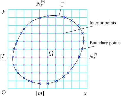
The moving least square procedure [26] is briefly described in this section. The domain of interest is discretised using a Cartesian grid as shown in Fig 1. On an
x-grid line, e.g. [l], consider a nodal point xi with its associated support domain, e.g.[xi−1,xi+1]for the case of 3-node local support. Let uh(x)be the approximation of the field variable u along this support domain and given by
uh(x) =
m
∑
j=0
pj(x)aj(x) =p¯T(x)a(x)¯ , (1)
where m is the number of terms of monomials, ¯a(x) a vector of coefficients and ¯
pT(x)a complete polynomial basis, given by
¯
a(x) = a0(x) a1(x) ... am(x) T
, (2)
¯
p(x) = p0(x) p1(x) ... pm(x) T
= 1 x x2 ... xm T. (3)
The expression for ¯a(x)can be obtained at each point x by minimizing the following weighted residual
J=
n
∑
I=1
W(x−xI) h
¯
pT(xI)a(x)¯ −u(I) i2
, (4)
where u(I) is the nodal value of the field variable u at x=xI, and n the number of nodes in the support domain of x where the weight function W(x−xI)6=0. In the present paper, the cubic spline weight function is used to construct MLS shape functions.
W(d) =
2 3−4d
2+4d3, d≤1 2 4
3−4d+4d2− 4 3d,
1
2<d≤1
0, d>1
where d=|x−xI|/dw and dw defines the size of the support domain. The mini-mization of the weighted residual J results in the following linear equation system
A(x)a(x) =¯ B(x)u¯, (6)
or
¯
a(x) =A(x)−1B(x)u¯, (7)
where
¯
u= u(1) u(2) ... u(n) T, (8)
A(x) =
n
∑
I=1
W(x−xI)p(x¯ I)p¯T(xI), (9)
B(x) = B1 B2 ... Bn , (10)
in which
BI=W(x−xI)p(x¯ I). (11)
Substituting (7) into (1), uhcan be expressed as
uh(x) =φ¯T(x)u¯, (12)
where ¯φis the vector of MLS shape functions and given by
¯
φ(x) = p¯TA−1B1 p¯TA−1B2 ... p¯TA−1Bn T
. (13)
It should be noted that the MLS shape functions do not satisfy the Kronecker-δ criterion, but possess a so-called partition of unity properties as follows.
n
∑
I=1 ¯
φI(x) =1. (14)
A new shape function possessing the Kronecker-δ function properties is created through a technique as described in the following section.
4 Moving least square - one dimensional integrated radial basis function net-works technique
networks (ns=5) is presented here. On an x-grid line[l], a global interpolant for the field variable at a grid point xiis sought in the form
u(xi) = n
∑
j=1 ¯
φj(xi)u[j](xi), (15)
whereφj¯ nj=1is a set of the partition of unity functions constructed using MLS
approximants, u[j](xi)is the nodal function value obtained from a local interpolant represented by a 1D-IRBF network[j], n is the number of nodes in the support do-main of xi. In (15), MLS approximants are presently based on linear polynomials, which are defined in terms of 1 and x. Relevant derivatives of u at xican be obtained by differentiating (15)
∂u(xi) ∂x =
n
∑
j=1
∂φj¯ (xi) ∂x u
[j](x
i) +φj¯ (xi)∂
u[j](xi) ∂x
!
, (16)
∂2u(x i) ∂x2 =
n
∑
j=1
∂2φj¯ (x i) ∂x2 u
[j](x i) +2∂
¯ φj(xi)
∂x
∂u[j](xi)
∂x +φj¯ (xi)
∂2u[j](x i) ∂x2
!
, (17)
where the values u[j](xi),∂u[j](xi)/∂x and∂2u[j](xi)/∂x2 are calculated from 1D-IRBFN networks with nsnodes.
4.1 One-dimensional IRBFN
Consider a segment [ j] with nsnodes on an x-grid line [l] as shown in Figure 2. The variation of the nodal function u[j] along this segment is sought in the IRBF form. The second-order derivative of u[j]is decomposed into RBFs; the RBF network is then integrated once and twice to obtain the expressions for the first-order derivative of u[j] and the function u[j]itself as follows.
∂2u[j](x) ∂x2 =
ns
∑
k=1
w(k)G(k)(x) =
ns
∑
k=1
w(k)H[(2k])(x), (18)
∂u[j](x)
∂x =
ns
∑
k=1
w(k)H[(1k])(x) +c1, (19)
u[j](x) =
ns
∑
k=1
w(k)H[(0k])(x) +c1x+c2, (20)
wherew(k) nk=s1are RBF weights to be determined;G(k)(x) ns
k=1= n
H[(2k])(x)ons
the multiquadrics G(k)(x) =p(x−x(k))2+a(k)2,a(k)- the RBF width determined as a(k)=βd(k),β a positive factor, and d(k)the distance from the kthcenter to its nearest neighbour.
It is more convenient to work in the physical space than in the network-weight space. The RBF coefficients including two integration constants can be transformed into the physically meaningful nodal variable values through the following relation
¯
u[j]=H¯
¯ w ¯ c , (21)
where ¯H is an ns×(ns+2)matrix and given by
H=
H[(01])(x1) H[(02])(x1) ... H[(0n]s)(x1) x1 1
H[(01])(x2) H( 2)
[0](x2) ... H( ns)
[0] (x2) x2 1
... ... ... ... ... ...
H[(01])(xns) H
(2)
[0](xns) ... H
(ns)
[0] (xns) xns 1
; (22)
¯
u[j]= (u(1),u(2), ...,u(ns))T; ¯w= (w(1),w(2), ...,w(ns))T and ¯c= (c
1,c2)T. There are two possible transformation cases.
For a segment [j] with only interior points: The direct use of (21) leads to an
underdetermined system of equations
¯
u[j]=H¯
¯ w ¯ c
=C¯
¯ w ¯ c , (23) or ¯ w ¯ c
=C¯−1u¯[j], (24)
where ¯C=H is the conversion matrix whose inverse can be found using the singu-¯
lar value decomposition (SVD) technique.
For a segment[j]with interior and boundary points: Owing to the presence of c1 and c2, one can add an additional equation of the form
f=K
¯ w ¯ c (25)
to equation system (21). In the case of Neumann boundary conditions, this subsys-tem can be used to impose a derivative boundary value at x=xb
f=∂u(xb)
∂x , (26)
K=h H[(11])(xb) H[(12])(xb) ... H[(1n]s)(xb) 1 0 i
The conversion system can be written as
¯
u[j] f = ¯ H K ¯ w ¯ c
=C¯
¯ w ¯ c , (28) or ¯ w ¯ c
=C¯−1
¯
u[j] f
. (29)
It can be seen that (24) is a special case of (29), where f is simply set to null. By substituting Equation (29) into Equations (18)-(20), the second- and first-order derivatives and the function of the variable u[j] are expressed in terms of nodal variable values as
∂2u[j](x) ∂x2 =
H[(21])(x),H[(22])(x), ...,H(ns)
[2] (x),0,0
¯
C−1
¯
u[j] f
, (30)
∂u[j](x)
∂x =
H[(11])(x),H[(12])(x), ...,H(ns)
[1] (x),1,0
¯
C−1
¯
u[j] f
, (31)
u[j](x) =H[(01])(x),H[(02])(x), ...,H(ns)
[0] (x),x,1
¯
C−1
¯
u[j] f
, (32)
or ∂2u[j](x)
∂x2 =d¯ T
2xu¯[j]+k2x(x), (33)
∂u[j](x)
∂x =d¯
T
1xu¯[j]+k1x(x), (34)
u[j](x) =d¯T
0xu¯[j]+k0x(x), (35)
where k0x,k1xand k2x are scalars whose values depend on x and a boundary value
f ; and ¯d0x,d¯1x and ¯d2x are known vectors of length ns.
By application of Equations (33) and (34) to ns nodes on the segment [ j], the second- and first-order derivatives of u[j]at node xi are determined as
∂2u[j](x i)
∂x2 =D¯2x(idk,:)u¯ [j]+¯k
2x(idk), (36)
∂u[j](xi)
∂x =D¯1x(idk,:)u¯
[j]+¯k
1x(idk), (37)
u[j](xi) =D¯0x(idk,:)u¯[j]+¯k0x(idk)=¯I(idk,:)u¯[j], (38)
in the local network[j]. It is noted that ¯D0x =¯I, where ¯I is an identity matrix of dimension ns×nsand ¯k0x=¯0. Therefore, the 1D-IRBFN shape function possesses the Kronecker-δ function properties.
4.2 Incorporation of MLS and 1D-IRBFN into the partition of unity framework
By substituting Equations (36)-(38) into Equations (15)-(17), the function u(xi)and its derivatives are expressed as
u(xi) = n
∑
j=1 ¯
m[0xj]u¯[j], (39)
∂u(xi) ∂x =
n
∑
j=1
¯
m[1xj]u¯[j]+k1x[j], (40)
∂2u(x i) ∂x2 =
n
∑
j=1
¯
m[2xj]u¯[j]+k[2xj], (41)
where
¯
m[0xj]=φj¯ (xi)¯I(idk,:), (42)
¯
m[1xj]=∂φj¯ (xi)
∂x ¯I(idk,:)+φj¯ (xi)D¯1x(idk,:), (43)
¯
m[2xj]=∂
2φj¯ (x i)
∂x2 ¯I(idk,:)+2 ∂φj¯ (xi)
∂x D¯1x(idk,:)+φj¯ (xi)D¯2x(idk,:), (44) k1x[j]=φ¯j(xi)¯k1x(idk), (45)
k2x[j]=2∂φ¯j(xi)
∂x ¯k1x(idk)+φ¯j(xi)¯k2x(idk). (46)
From Equations (14), (39) and (42), one can see that the LMLS-1D-IRBFN shape function possesses the Kronecker-δ function properties.
Equations (40) and (41) can be expressed as ∂u(xi)
∂x =m¯
[i] 1xu¯[
i]+k[i]
1x, (47)
∂2u(x i) ∂x2 =m¯
[i] 2xu¯
[i]+k[i]
2x, (48)
where ¯u[i]= u(1),u(2), ...,u(nr)T, nrthe number of nodes in the network[i], k[i]
1xand
k2x[i] are known scalars, and ¯m1x[i] and ¯m[2xi] are known vectors of length nr, defined by
¯
m[1xi](id j)=m¯[1xi](id j)+m¯[1xj], j=1,2, ...,n (49)
¯
in which id j is the index vector mapping the location of nodes of the local network
[j]to that in the LMLS-1D-IRBF network[i].
The values of first- and second-order derivatives of u with respect to x at the nodal points on the grid line[l]are given by
∂uˆ ∂x =Mˆ
[l] 1xuˆ
[l]+ˆk[l]
1x, (51)
∂2uˆ ∂x2 =Mˆ
[l] 2xuˆ
[l]+ˆk[l]
2x, (52)
where
ˆ
u=u(1),u(2), ...,u(nl)T, (53)
ˆ
M[1xl](i,idi)=m¯[1xi], (54)
ˆ
M[2xl](i,idi)=m¯[2xi], (55)
ˆk[l] 1x(i)=k
[i]
1x, (56)
ˆk[l] 2x(i)=k
[i]
2x, (57)
in which nl is the number of nodes on the grid line[l], and idi the index vector mapping the location of nodes of the local network[i]to that in the grid line[l].
The values of first- and second-order derivatives of u with respect to x at the nodal points over the problem domain are given by
∂u˜
∂x =M˜1xu˜+˜k1x, (58)
∂2u˜
∂x2 =M˜2xu˜+˜k2x, (59)
where
˜
u=u(1),u(2), ...,u(Nip)T, (60)
∂u˜ ∂x =
∂u(1)
∂x ,
∂u(2)
∂x , ...,
∂u(Nip)
∂x
!T
, (61)
∂2u˜ ∂x2 =
∂2u(1) ∂x2 ,
∂2u(2) ∂x2 , ...,
∂2u(Nip)
∂x2 !T
, (62)
matrices ˜M1xand ˜M2xand the vectors ˜k1xand ˜k2xare formed as follows.
˜
M1x(idl,idl)=Mˆ[1xl], (63)
˜
M2x(idl,idl)=Mˆ[2xl], (64)
˜k1x(idl)=ˆk[1xl], (65)
˜k2x(idl)=ˆk[2xl], (66)
in which idl is the index vector mapping the location of nodes on the grid line[l]to that in the whole grid.
Similarly, the values of the second- and first-order derivatives of u with respect to
y at the nodal points over the problem domain are given by
∂u˜
∂y =M˜1yu˜+˜k1y, (67)
∂2u˜
∂y2 =M˜2yu˜+˜k2y. (68)
5 Governing equations for two-dimensional incompressible viscous flows
In this work we limit the analysis to two-dimensional problems andthe governing equations for incompressible viscous flows can therefore be written in terms of stream functionψ and vorticityω as [27]
∂2ψ ∂x2 +
∂2ψ
∂y2 =−ω, (69)
1
Re
∂2ω ∂x2 +
∂2ω ∂y2
=∂ω
∂t +
∂ψ
∂y
∂ω ∂x −
∂ψ ∂x
∂ω ∂y
, (70)
where Re is the Reynolds number, t the time, and(x,y)T the position vector. The
x and y components of the velocity vector can be defined in terms of the stream
function as
u=∂ψ
∂y, (71)
v=−∂ψ
6 LMLS-1D-IRBFN discretisation of governing equations for incompressible viscous flows
The domain of interest is discretised using uniform Cartesian grids. With the backward Euler scheme for time discretisation, Equations (69) and (70) can be expressed as
∂2ψ(n+1) ∂x2 +
∂2ψ(n+1) ∂y2 =−ω
(n), (73)
∆t Re
∂2ω(n+1) ∂x2 +
∂2ω(n+1) ∂y2
!
−ω(n+1)=−ω(n)+∆t ∂ψ(n) ∂y
∂ω(n) ∂x −
∂ψ(n) ∂x
∂ω(n) ∂y
!
,
(74)
where the superscripts (n)and (n+1)denote the time levels and∆t the time
dis-cretisation step.
Making use of (58), (59), (67) and (68) and collocating the governing equations (73) and (74) at the interior points result in
˜
E1ψ˜(n+1)=RHS1, (75)
˜
E2ω˜(n+1)=RHS2, (76)
where
˜
E1=M˜2x+M˜ 2y, (77)
RHS1=−ω(n)− ˜k2xψ+˜k2yψ
, (78)
˜
E2= ∆t
Re M˜2x+M˜2y−˜I
, (79)
RHS2=−ω(n)−Re∆t ˜k2xω+˜k2yω
+∆thM˜1yψ˜(n)+˜k1y(n)ψ
.M˜ 1xω˜(n)+˜k(n) 1xω
−M˜1xψ˜(n)+˜k(n) 1xψ
.M˜1yω˜(n)+˜k(n) 1yω
i ,
(80)
in which ˜k1xψ,˜k2xψ,˜k1yψ,˜k2yψ,˜k1xω,˜k2xω,˜k1yω and ˜k2yω are known vectors of length
Nip.
The nonlinear system of equations (75) and (76) is solved using the pseudo-time stepping procedure as follows:
• Step 1: Guess the initial solution of vorticityω.
• Step 3: Compute the vorticity boundary conditions and the convection terms explicitly.
• Step 4: Solve (76) forω.
• Step 5: Check convergence criterion forω s
Nip ∑ i=1
ω(t+1)
i −ω
(t) i
2
s Nip
∑ i=1
ω(t+1)
i 2
<T OL, (81)
where T OL is a given tolerance and presently set to be 10−12. If not con-verged, return to step 2. Otherwise, stop.
7 Numerical results and discussion
Several examples are investigated here to study the performance of the present method. The domains of interest are discretised using Cartesian grids. By using the LMLS-1D-IRBFN method to discretise governing equations and the LU decompo-sition technique to solve the resultant sparse system of simultaneous equations, the computational cost and data storage requirements are reduced. For the purpose of CPU times comparisons, all related computations are carried out on a single 2.4
GHz processor machine with 4 GB RAM.
7.1 Example 1: Two-dimensional Poisson equation in a square domain
The present method is first verified through the solution of the following 2D Poisson equation
∂2u ∂x2 +
∂2u
∂y2 =0, (82)
defined on a square domain 0≤x,y≤1 and subject to Dirichlet boundary condi-tions. The problem has the following exact solution
uE = 1
sinh(π)sin(πx)sinh(πy). (83)
A uniform grid of Nx×Nyis employed to discretise the problem domain. Two cases of boundary conditions are considered as follows.
• Case 2: Dirichlet boundary conditions are imposed along two horizonal edges and Neumann boundary conditions are imposed along two vertical edges.
These boundary conditions can be derived from the exact solution. The proposed LMLS-1D-IRBFN method with the following two approaches is considered.
• Approach 1: n=3 and ns=3, called LMLS-1D-IRBFN-3-node.
• Approach 2: n=3 and ns=5, called LMLS-1D-IRBFN-5-node.
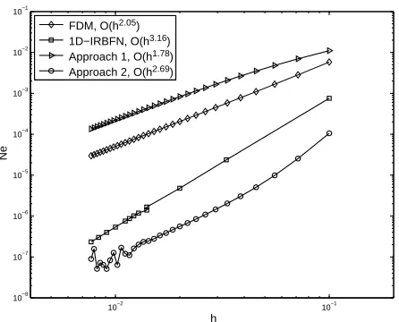
Figure 3 presents the grid convergence study for Case 1 for the two approaches in comparison with those ofFDM with central-difference scheme andthe 1D-IRBFN method. The convergence study for Case 2 for the two approaches in comparison with those of the 1D-IRBFN method is shown in Figure 4. The convergence be-haviours ofFDM,1D-IRBFN, Approach 1 and Approach 2 for Case 1 areO(h2.05), O(h3.16), O(h1.78) and O(h2.69), respectively. The convergence behaviour of 1D-IRBFN, Approach 1 and Approach 2 for Case 2 areO(h1.98), O(h1.84) and O(h1.89), respectively. The numerical results show that the LMLS-1D-IRBFN-5-node is much more accurate than FDM andLMLS-1D-IRBFN-3-node, and slightly bet-ter than those of its global counbet-terpart, i.e. 1D-IRBFN method.
in Figure 3 and Table 2, the present Approach 2 with grid=21×21 yields better accuracy (Ne=6.88e−6) in 0.88 seconds than the FDM with grid=121×121 (Ne=3.49e−5) in 1.74 seconds.
Approach 2 yields much more accurate results than Approach 1 and FDM with central-difference scheme and is significantly more efficient than 1D-IRBFN in terms of computational cost, as grid density increases. Therefore, the remaining examples will be investigated using Approach 2, i.e. LMLS-1D-IRBFN-5-node.
7.2 Example 2: Two-dimensional Poisson equation in a square domain with a
circular hole
This example is concerned with the following 2D Poisson equation
∂2u ∂x2 +
∂2u
∂y2 =−8π
2sin(2πx)sin(2πy), (84)
defined on a square domain with a circular hole as shown in Figure 5 and subject to Dirichlet boundary conditions. The problem has the following exact solution
uE =sin(2πx)sin(2πy), (85)
from which the boundary values of u can be derived.
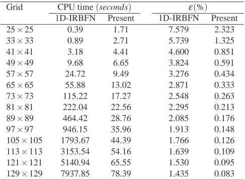
The grid convergence study for LMLS-1D-IRBFN and 1D-IRBFN methods is pre-sented in Figure 6. Table 4 describes the relative error norms (Ne) and condi-tion number (cond) of the present method in comparison with those of 1D-IRBFN method. The numerical results showed that the present method is not as accurate as the 1D-IRBFN method, but has a higher convergence rate (error norm of O(h3.70)) than the 1D-IRBFN method (error norm of O(h3.00)). Table 5 presents the com-parison of CPU time and percentage of nonzero elements of the system matrix (ε) between the 1D-IRBFN and LMLS-1D-IRBFN methods. The present method is much more efficient than the 1D-IRBFN method in terms of CPU time (e.g. 101.3 times for a grid of 129×129) and memory requirements (e.g. 17.2 times for a grid of 129×129), thus the grid size can be refined to obtain more accurate solutions as shown in Figure 6.
However, at this higher level of accuracy, the local convergence rate decreases, causing a lower overall convergence rate as described above.
7.3 Example 3: Lid-driven cavity flow
The cavity is taken to be a unit square with the lid sliding from left to right at a unit velocity as shown in Figure 7. The boundary conditions for stream functionψ are defined by
ψ=0, on x=0,x=1,y=0,y=1, (86)
∂ψ
∂x =0, on x=0,x=1, (87)
∂ψ
∂y =0, on y=0, (88)
∂ψ
∂y =1, on y=1. (89)
It is noted that only the Dirichlet boundary conditions (86) are used for solving (69), while the Neumann boundary conditions (87)-(89) are used to derive computational vorticity boundary conditions for solving (70).
It is well-known that the major difficulties of lid-driven cavity flow simulation are: (i) the presence of singularities at two of the corners, which makes it difficult to pre-dict the solution accurately; and (ii) the dominant convection terms, when dealing with high Re, which can cause oscillatory solutions if an improper scheme is used or computational grids are not sufficiently refined. The grid convergence study is first conducted for the lid-driven cavity flow problem with Re of 1000 using fol-lowing two approaches.
• Approach 1: The convection terms are calculated using LMLS-1D-IRBFN technique.
• Approach 2: The convection terms are calculated using global 1D-IRBFN technique.
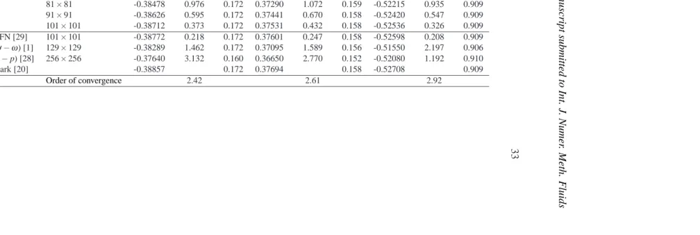
(ε= (Vm−Vs)×100/Vs) of the extremal velocities (Vm) based on the corresponding spectral benchmark solutions (Vs) [20] are given. It can be seen that these errors reduce with increasing grid densities. The orders of convergence are 2.42, 2.61 and 2.92 for the minimum horizontal velocity umin, the maximum vertical velocity
vmax and the minimum vertical velocity vmin along the center lines, respectively. The present results for a grid of 101×101 are more accurate than those of FDMs with more refined grids [1, 28], but less than those of 1D-IRBFN [29]. Table 7 describes comparisons of the number of nonzero elements per row of the system matrix (Nnzpr), number of iterations (Niteration) and total CPU time (Ttotal) required to obtain the converged solution with T OL=10−12. The time step∆t is set to be 5×10⁻³for all cases. Note that for a given grid size the present approach is slower than the FDM. However, the present approach achieves a given level of accuracy with a coarser grid and hence more efficient. For example, as shown in Tables 6 and 7, the present approach with grid=81×81 yields better accuracy in 1559.77 seconds than the FDM with grid=129×129 in 1733.02 seconds.
The corresponding grid convergence study for Approach 2 is given in Table 8. The orders of convergence are 3.80, 3.26 and 4.26 for umin, vmaxand vmin, respectively. It is interesting to see that Approach 2 yields more accurate results than Approach 1 and the 1D-IRBFN method,and the convergence orders of Approach 2 are higher than those of Approach 1. Approach 2 is employed to study the cases with high Reynolds numbers (Re=3200 and 7500). The contours of stream function and vorticity of the flow field inside the cavity atRe=1000,3200 and 7500 are shown in Figure 8. The vertical and horizontal velocities along the horizontal and vertical center lines atRe=1000,3200 and 7500 are given in Figure 9. These figures show that the current results are in good agreement with benchmark solutions of Ghia et al. [1] and Botella and Peyret [20].
7.4 Example 4: Flow past a circular cylinder
The steady flow past a circular cylinder at low Re numbers are considered in this section, where Re=U0D/ν, U0 is the far-field inlet velocity taken to be 1, D the diameter of the cylinder taken to be 1,ν the kinematic viscosity. The top, bottom, inlet and outlet boundaries are positioned at a distance of 20D,20D,10D and 30D away from the cylinder, respectively, as shown in Figure 10. These distances are large enough to assume that the far-field flow behaves as a potential flow [22] and the far-field stream functionψf arcan be defined by
ψf ar=U 0y
1− D
2
4(x2+y2)
The boundary conditions for stream function and vorticity are given by
ψ=ψf ar,ω=0, onΓ1,Γ2,Γ3, (91)
∂ψ ∂x =0,
∂ω
∂x =0, onΓ4, (92)
ψ=0,∂ψ
∂n =0, onΓw. (93)
where n is the direction normal to the cylinder surface as shown in Figure 11. The values of the vorticity on the circular boundaryΓwcan be computed as
ωw=−
∂2ψw ∂x2 +
∂2ψw ∂y2
(94)
where the subscript w is used to denote quantities on the circular boundary. A formula of Le-Cao et al. [30] is employed here to derive the vorticity boundary conditions at boundary points on x- and y-grid lines as follows.
ω(x)
w =−
" 1+
tx
ty
2#∂2ψw
∂x2 −qy, (95)
ω(y)
w =−
" 1+
ty
tx
2#∂2ψw
∂y2 −qx, (96)
where qxand qy are known quantities defined by
qx=−
ty
t2 x
∂2ψw ∂y∂s +
1
tx ∂2ψw
∂x∂s, (97)
qy=−
tx
t2 y
∂2ψw ∂x∂s +
1
ty ∂2ψw
∂y∂s, (98)
in which tx =∂x/∂s,ty =∂y/∂s and s is the direction tangential to the cylinder surface (Figure 11).
Calculation of drag and pressure coefficients
For viscous flow, the forces acting on the body come from two sources including pressure and friction. For the case of flow past a circular cylinder, the drag FDand its coefficient CDcan be defined by
FD=R 2π Z
0
µR∂ω
∂n −µω
sinθdθ, (99)
CD=
FD
where R is the radius of the cylinder,ρ fluid density andµ the dynamic viscosity. The dimensionless pressure coefficient is given by
Cp(θ) =
p(θ)−p0 1/2ρU2
0
, (101)
where p0 is the far-field inlet pressure, and p(θ) is the pressure on the cylinder surface at angleθ, evaluated as [31]
p(θ) = (p0+1/2ρU02)− d0
Z
R
µ
r
∂ω ∂θ
θ=0 dr−R θ Z
0 µ∂ω
∂n
r=R dθ, (102)
in which d0is the distance from the cylinder center to the inlet boundary.
Non-overlapping domain decomposition technique
As described in Section 5, the relevant governing equations are of Poisson type. Thus, consider the following Poisson problem in a domainΩwith Dirichlet bound-ary condition on the boundbound-ary∂Ω
∆u= f(x,y) inΩ (103)
u=b on∂Ω (104)
It is noted that the Neumann boundary conditions (92) can be imposed directly through the conversion process (26-29). Therefore, we just need to consider the Poisson problem with Dirichlet boundary condition here.
Without loss of generality, the domain of interestΩis partitioned into just two non-overlapping subdomainsΩ1and Ω2 as shown in Figure 12. The Poisson problem can be reformulated in the equivalent multi-domain form as follows [33].
∆u[1]= f[1] inΩ
1 (105)
u=b[1] on∂Ω1∩∂Ω (106)
∆u[2]= f[2] inΩ
2 (107)
u=b[2] on∂Ω2∩∂Ω (108)
u[1]=u[2] onΓ (109)
∂u[1] ∂n =
∂u[2]
whereΓis the interface betweenΩ1andΩ2,∂Ω1and∂Ω1are the boundaries of the subdomainsΩ1 andΩ2, respectively, and the superscript [·]denotes a subdomain. Equations (109) and (110) are the transmission conditions for u[1] and u[2] on the interface Γ. By solving the system of Equations (105-110), one can obtain the interface values uΓ, and the subdomain solutions u[1] and u[2].
We now describe an algorithm for solving the system of Equations (105-110) as follows. Let the subscripts ip,bp and f b represent the location indices of interior
points, known boundary points and interface points over a subdomain, respectively;
N, Nip, Nbpand Nf p are the total number of points, the number of interior points, known boundary points and interface points of a subdomain, respectively.
System of Equations (105-110) are written in matrix form as follows.
˜
E[1]u˜[1]=RHS[1], (111)
˜
u[(1bp] )=u[b1], (112)
˜
E[2]u˜[2]=RHS[2], (113)
˜
u[(2bp] )=u[b2], (114)
˜
u([1f p] )=u˜([2f p] )=uΓ, (115)
D[1]u˜[1]=D[2]u˜[2], (116)
where ˜E[1] and ˜E[2] are the known matrices of dimension(Nip[1]×N[1])and(Nip[2]×
N[2]), respectively; ˜u[1] and ˜u[2] are field variable vectors of length N[1] and N[2], respectively; RHS[1], RHS[2], u[b1]and ub[2]are the known vectors of length Nip[1], Nip[2],
Nbp[1] and Nbp[2], respectively; uΓ unknown vector of length Nf p; and D[1] and D[2]the known matrices of dimension(Nf p×N[1])and(Nf p×N[2]), respectively.
From (111), (112) and (115), one is able to obtain the following expression
h
˜
E([1:,ip] ) E˜([:1,bp] ) E˜([1:,]f p) i
˜
u[(1ip]) u[b1]
uΓ
=RHS[1] (117)
or
˜
u[(1ip])=A[1]+B[1]uΓ (118)
where
A[1]=E˜[1] (:,ip)
−1
RHS[1]−E˜[1] (:,bp)u
[1]
b
, (119)
B[1]=−E˜[1] (:,ip)
−1 ˜
Similarly, from (113), (114) and (115), the interior values of the subdomainΩ2is given by
˜
u[(2ip])=A[2]+B[2]uΓ (121)
where
A[2]=E˜[2]
(:,ip)
−1
RHS[2]−E˜[2]
(:,bp)u [2]
b
, (122)
B[2]=−E˜([2:,ip] )−
1 ˜
E([2:,]f p). (123)
Equation (116) can be expressed as
h
D[(1:,ip] ) D([1:,bp] ) D[(1:,]f p)
i
˜
u[(1ip]) u[b1]
uΓ
=h D([2:,ip] ) D[(2:,bp] ) D[(2:,]f p)
i
˜
u[(2ip]) u[b2]
uΓ .
(124)
By substituting Equations (118) and (121) into (124), the interface values uΓ are determined as
uΓ=
−D[(1:,ip] )A[1]−D[(1:,bp] )u[b1]+D[(2:,ip] )A[2]+D[(2:,bp] )u[b2] D[(1:,ip] )B[1]+D[1]
(:,f p)−D
[2]
(:,ip)B[2]−D [2] (:,f p)
. (125)
By substituting (125) into (118) and (121), one can obtain the subdomain solutions ˜
u[(1ip])and ˜u[(2ip]).
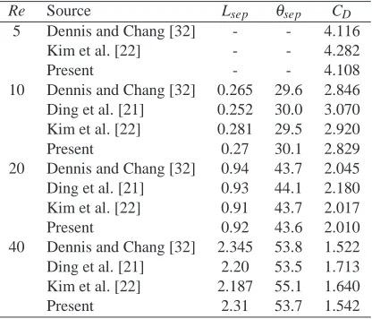
vortices and the separated region behind the cylinder are formed. The length of the wake is measured from the rear of the cylinder to the end of the separated region, while the angle of separation is defined at the point where the vorticity vanishes. Table 9 presents the length of the wake behind the cylinder (Lsep), the separation angle (θsep) and the drag coefficient (CD) for Re numbers of 5, 10, 20 and 40. The comparison of vorticity and pressure coefficient distribution on the cylinder surface in the case of Re numbers of 5, 10, 20 and 40 are given in Figure 15 and 16, respec-tively. It can be seen that the present numerical results are in good agreement with other published results. The contours of stream function and vorticity of the flow field around the cylinder are shown in Figure 17.
8 Conclusions
A local MLS-1D-IRBFN method is proposed for solving incompressible viscous flow problems in terms of stream function and vorticity. The present approach is based on the PU concept and incorporates the MLS and 1D-IRBFN methods. The LMLS-1D-IRBFN approach offers the same order of accuracy as the 1D-IRBFN method, while the system matrix is more sparse than that of the 1D-IRBFN, which helps reduce the computational cost significantly as discussed earlier. The LMLS-1D-IRBFN shape function possesses the Kronecker-δ property which allows an exact imposition of the essential boundary condition. Cartesian grids are used to discretise both rectangular and irregular problem domains. The numerical results for the lid-driven cavity flows at high Re numbers showed that the calculation of convection terms using the global 1D-IRBFN technique are more accurate than the one using the IRBFN technique. The combination of the LMLS-1D-IRBFN method and a domain decomposition technique is successfully developed for solving a larger problem. The obtained numerical results for both cases of lid-driven cavity flow and flow past a circular cylinder are in good agreement with other published results available in the literature.The present method can be used to handle problems with irregular domains, while the standard finite different method cannot be applied directly at the grid points near the boundary of irregular domains. Owing to the use of integrated RBFN for local approximation, the present method appears to be more accurate than the FDM with central-difference scheme. Owing to the use of a fixed Cartesian grid, the present method is expected to be more efficient than the conventional FDM, FVM and FEM when solving problems with moving boundary.
comments.
References
[1]Ghia U, Ghia KN, Shin CT. High-Re solutions for incompressible flow using the Navier-Stokes equations and a multigrid method. Journal of Computational
Physics 1982; 48:387-411.
[2]Leonard BP. A stable and accurate convective modelling procedure based on quadratic upstream interpolation. Computer methods in applied mechanics and
engineering 1979; 19:59-98.
[3]Brooks AN, Hughes TJR. Streamline upwind/Petrov-Galerkin formulations for convection domainted flows with particular emphasis on the incompressible Navier-Stokes equations. Computer methods in applied mechanics and
engineer-ing 1982; 32:199-259.
[4]Lin H, Atluri SN. Meshless local Petrov-Galerkin (MLPG) method for convection-diffusion problems. Computer Modeling in Engineering & Sciences 2000; 1(2):45-60.
[5]Lin H, Atluri SN. The meshless local Petrov-Galerkin (MLPG) method for solv-ing incompressible Navier-Stokes equations. Computer Modelsolv-ing in Engineersolv-ing
& Sciences 2001; 2(2):117-142.
[6]Babuˆska I. Error-bounds for finite element method. Numerische Mathematik 1971; 16(4):322-333.
[7]Kansa EJ. Multiquadrics - A Scattered Data Approximation Scheme with Appli-cations to Computational Fulid-Dynamics - II: Solutions to parabolic, Hyperbolic and Elliptic Partial Differential Equations. Computers & Mathematics with
Appli-cations 1990; 19(8/9):147-61.
[8]Park SH, Youn SK. The least-squares meshfree method. International Journal
for Numerical Methods in Engineering 2001; 52:997-1012.
[9]Zhang XK, Kwon KC, Youn SK. The least-squares meshfree method for the steady incompressible viscous flow. Journal of Computational Physics 2005; 206:182-207.
[11]Arzani H, Afshar MH. Solving Poisson’s equations by the discrete least squares meshless method. In Boundary Elements and Other Mesh Reduction Methods
XXVIII. WIT Pres: Skiathos, Greece, 2006; 23-32.
[12]Firoozjaee AR, Afshar MH. Steady-state solution of incompressible Navier-Stokes equations using discrete least-squares meshless method. Intenational
Jour-nal for Numerical Methods in Fluids 2011; 67:369-382.
[13]Lee CK, Liu X, Fan SC. Local multiquadric approximation for solving bound-ary value problems. Computational Mechanics 2003; 30:396-409.
[14]Šarler B, Vertnik R. Meshfree explicit local radial basis function collocation method for diffusion problems. Computers and Mathematics with Applications 2006; 51:1269-1282.
[15]Babuˆska I, Melenk JM. The partition of unity method. International Journal
for Numerical Methods in Engineering 1997; 40:727-758.
[16]Krysl P, Belytschko T. An efficient linear-precision partition of unity basis for unstructured meshless methods. Communications in Numerical Methods in
Engi-neering 2000; 16:239-255.
[17]Shepard D. A two dimensional interpolation function for irregularly spaced data. In Proceedings of the 23rd National Conference ACM. ACM: New York 1968; 517-523.
[18]Chen JS, Hu W, Hu HY. Reproducing kernel enhanced local radial basis col-location method. International Journal for Numerical Methods in Engineering 2008; 75:600-627.
[19]Le PBH, Rabczuk T, Mai-Duy N, Tran-Cong T. A moving IRBFN-based integration-free meshless method. Computer Modeling in Engineering &
Sci-ences 2010; 61(1):63-109.
[20]Botella O, Peyret R. Benchmark spectral results on the lid-driven cavity flow.
Computers & Fluids 1998; 27(4):421-433.
[21]Ding H, Shu C, Yeo KS, D. Xu. Simulation of incompressible viscous flows past a circular cylinder by hybrid FD scheme and meshless least square-based fi-nite difference method. Computer Methods in Applied Mechanics and
Engineer-ing 2004; 193:727-744.
[22]Kim Y, Kim DW, Jun S, Lee JH. Meshfree point collocation method for the stream-vorticity formulation of 2D incompressible Navier-Stokes equations.
[23]Mai-Duy N, Tanner RI. A Collocation Method based on One-Dimensional RBF Interpolation Scheme for Solving PDEs. International Journal of
Numer-ical Methods for Heat & Fluid Flow 2007; 17(2):165-186.
[24]Mai-Duy N, Tran-Cong T. Numerical solution of differential equations using multiquadric radial basis function networks. Neural Networks 2001; 14:185-199.
[25]Ngo-Cong D, Mai-Duy N, Karunasena W, Tran-Cong T. Free vibration analy-sis of laminated composite plates based on FSDT using one-dimensional IRBFN method. Computers & Structures 2011; 89:1-13.
[26]Liu GR. Meshfree Methods: Moving beyond the Finite Element Method. CRC Press LLC: Boca Raton, Florida, 2003.
[27]Glowinski R. Finite Element Methods for Incompressible Viscous Flows. In
Handbook of Numerical Analysis, Vol. 9, Ciarlet PG and Lions JL (eds).
North-Holland: Amsterdam, 2003.
[28]Bruneau CH, Jouron C. An efficient scheme for solving steady incompressible Navier-Stokes equations. Journal of Computational Physics 1990; 89(2):389-413.
[29]Mai-Duy N, Tran-Cong T. Integrated radial-basis-function networks for com-puting Newtonian and non-Newtonian fluid flows. Computers & Structures 2009; 87:642-650.
[30]Le-Cao K, Mai-Duy N, Tran-Cong T. An effective integrated-RBFN Cartesian-grid discretization for the stream function-vorticity-temperature formulation in nonrectangular domains. Numerical Heat Transfer, Part B 2009; 55:480-502.
[31]Muralidhar K, Sundararajan T. Computational fluid flow and heat transfer. In
IIT Kanpur Series of Advanced Texts. Narosa Publishing House: New Delhi, 1995
pages 219-220.
[32]Dennis SCR, Chang GZ. Numerical solutions for steady flow past a circu-lar cylinder at Reynolds number up to 100. Journal of Fluid Mechanics 1970; 42(3):471-489.
[33]Quarteroni A, Valli A. Domain Decomposition Methods for Partial Differential
M
a
n
u
sc
ri
p
t
su
b
m
itt
ed
to
In
t.
J.
N
u
m
er
.
M
et
h
.
F
lu
id
s
2
9
[image:29.595.142.584.208.344.2]M
a
n
u
sc
ri
p
t
su
b
m
it
te
d
to
In
t.
J.
N
u
m
er
3
[image:30.595.211.775.307.465.2]0
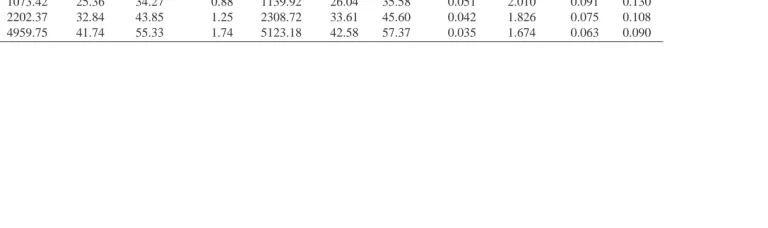
Table 2: Poisson equation in a square domain subject to Dirichlet boundary conditions: comparison (with FDM and
1D-IRBFN) of CPU time and percentage of nonzero elements of the system matrix (ε). Note that for a given grid size the
present Approach 2 is slower than the FDM. However, the present Approach 2 achieves a given level of accuracy with a coarser grid and hence more efficient. For example, as shown in Figure 3, the present Approach 2 with grid=21×21 yields better accuracy (Ne=6.88e−6) in 0.88 seconds than the FDM with grid=121×121 (Ne=3.49e−5) in 1.74 seconds.
Grid CPU time(seconds)for all shape functions Total CPU time(seconds) ε(%)
FDM 1D-IRBFN App. 1 App. 2 FDM 1D-IRBFN App. 1 App. 2 FDM 1D-IRBFN App. 1 App. 2
11×11 0.00 0.03 0.12 0.22 0.00 0.05 0.18 0.23 5.624 20.988 9.465 12.757
21×21 0.00 0.06 0.53 0.86 0.01 0.10 0.54 0.88 1.327 10.249 2.318 3.251
31×31 0.01 0.39 1.31 2.05 0.02 0.58 1.33 2.08 0.578 6.778 1.021 1.447
41×41 0.03 2.12 2.54 3.83 0.05 2.85 2.62 3.97 0.322 5.062 0.571 0.814
51×51 0.05 8.58 4.35 6.34 0.09 10.71 4.46 6.58 0.205 4.040 0.365 0.521
61×61 0.10 25.98 6.82 9.71 0.16 30.86 6.99 10.00 0.142 3.361 0.253 0.362
71×71 0.18 66.68 10.01 14.02 0.25 77.73 10.24 14.49 0.104 2.878 0.185 0.266
81×81 0.30 169.14 14.08 19.44 0.40 190.49 14.40 20.14 0.079 2.516 0.142 0.203
91×91 0.46 462.68 19.15 26.11 0.62 502.23 19.67 26.90 0.063 2.235 0.112 0.161
101×101 0.69 1073.42 25.36 34.27 0.88 1139.92 26.04 35.58 0.051 2.010 0.091 0.130
111×111 1.00 2202.37 32.84 43.85 1.25 2308.72 33.61 45.60 0.042 1.826 0.075 0.108
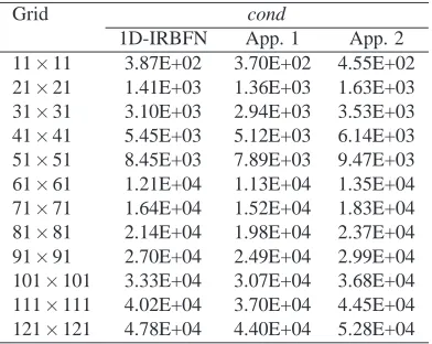
Table 3: Poisson equation in a square domain subject to Dirichlet and Neumann boundary conditions: comparison condition number (cond).
Grid cond
1D-IRBFN App. 1 App. 2 11×11 3.87E+02 3.70E+02 4.55E+02 21×21 1.41E+03 1.36E+03 1.63E+03 31×31 3.10E+03 2.94E+03 3.53E+03 41×41 5.45E+03 5.12E+03 6.14E+03 51×51 8.45E+03 7.89E+03 9.47E+03 61×61 1.21E+04 1.13E+04 1.35E+04 71×71 1.64E+04 1.52E+04 1.83E+04 81×81 2.14E+04 1.98E+04 2.37E+04 91×91 2.70E+04 2.49E+04 2.99E+04 101×101 3.33E+04 3.07E+04 3.68E+04 111×111 4.02E+04 3.70E+04 4.45E+04 121×121 4.78E+04 4.40E+04 5.28E+04
Table 4: Poisson equation in a square domain with a circular hole subject to Dirich-let boundary conditions: comparison of relative error norm (Ne) and condition number (cond).
Grid Ne cond
[image:31.595.125.381.541.720.2]Table 5: Poisson equation in a square domain with a circular hole subject to Dirich-let boundary conditions: comparison of CPU time and percentage of nonzero ele-ments of the system matrix (ε).
Grid CPU time(seconds) ε(%)
1D-IRBFN Present 1D-IRBFN Present
25×25 0.39 1.71 7.579 2.323
33×33 0.89 2.71 5.739 1.325
41×41 3.18 4.41 4.600 0.851
49×49 9.68 6.65 3.824 0.591
57×57 24.72 9.49 3.276 0.434
65×65 55.88 13.02 2.871 0.333
73×73 115.22 17.27 2.548 0.263
81×81 222.04 22.56 2.295 0.213
89×89 464.42 28.76 2.085 0.176
97×97 946.15 35.96 1.913 0.148
105×105 1793.67 44.39 1.766 0.126
113×113 3153.54 54.16 1.639 0.109
121×121 5140.94 65.55 1.530 0.095
M
a
n
u
sc
ri
p
t
su
b
m
itt
ed
to
In
t.
J.
N
u
m
er
.
M
et
h
.
F
lu
id
s
3
3
Present 21×21 -0.33342 14.193 0.333 0.27403 27.301 0.220 -0.34690 34.184 0.827 31×31 -0.33043 14.962 0.202 0.32097 14.848 0.172 -0.43390 17.678 0.888 41×41 -0.35408 8.876 0.183 0.34304 8.993 0.165 -0.47541 9.804 0.901 51×51 -0.36903 5.029 0.177 0.35730 5.211 0.162 -0.49891 5.345 0.906 61×61 -0.37750 2.848 0.174 0.36561 3.006 0.160 -0.51164 2.930 0.907 71×71 -0.38218 1.644 0.173 0.37027 1.769 0.159 -0.51846 1.635 0.908 81×81 -0.38478 0.976 0.172 0.37290 1.072 0.159 -0.52215 0.935 0.909 91×91 -0.38626 0.595 0.172 0.37441 0.670 0.158 -0.52420 0.547 0.909 101×101 -0.38712 0.373 0.172 0.37531 0.432 0.158 -0.52536 0.326 0.909 1D-IRBFN [29] 101×101 -0.38772 0.218 0.172 0.37601 0.247 0.158 -0.52598 0.208 0.909 FDM (ψ−ω) [1] 129×129 -0.38289 1.462 0.172 0.37095 1.589 0.156 -0.51550 2.197 0.906 FDM (u−p) [28] 256×256 -0.37640 3.132 0.160 0.36650 2.770 0.152 -0.52080 1.192 0.910
Benchmark [20] -0.38857 0.172 0.37694 0.158 -0.52708 0.909
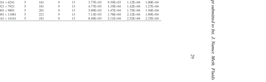
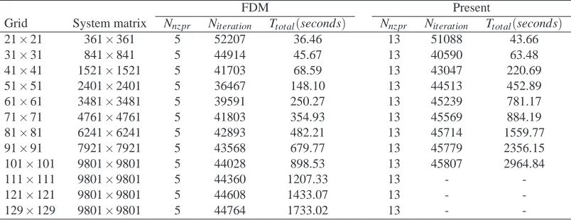
[image:33.595.91.637.191.360.2]Table 7:Lid-driven cavity flow, Re=1000: comparisons of the number of nonzero elements per row of the system matrix (Nnzpr), number of iterations (Niteration) and total CPU time (Ttotal) required to obtain the converged solution with T OL=10−12. The time step∆t is set to be 5×10⁻³for all cases. Note that for a given grid size the present approach is slower than the FDM. However, the present approach achieves a given level of accuracy with a coarser grid and hence more efficient. For example, as shown in Table 6, the present approach with grid=81×81 yields better accuracy in 1559.77 seconds than the FDM with grid=129×129 in 1733.02 seconds.
FDM Present
Grid System matrix Nnzpr Niteration Ttotal(seconds) Nnzpr Niteration Ttotal(seconds)
21×21 361×361 5 52207 36.46 13 51088 43.66
31×31 841×841 5 44914 45.67 13 40590 63.48
41×41 1521×1521 5 41703 68.59 13 43047 220.69
51×51 2401×2401 5 36467 148.10 13 44513 452.89
61×61 3481×3481 5 39591 250.27 13 45239 781.17
71×71 4761×4761 5 41803 354.93 13 45569 884.19
81×81 6241×6241 5 42893 482.21 13 45714 1559.77
91×91 7921×7921 5 43568 679.77 13 45779 2356.15
101×101 9801×9801 5 44028 898.53 13 45807 2964.84
111×111 9801×9801 5 44360 1207.33 13 -
-121×121 9801×9801 5 44608 1433.07 13 -
-M
a
n
u
sc
ri
p
t
su
b
m
itt
ed
to
In
t.
J.
N
u
m
er
.
M
et
h
.
F
lu
id
s
3
5
Present 21×21 -0.30543 21.397 0.223 0.29460 21.844 0.181 -0.39550 24.963 0.866 31×31 -0.35522 8.583 0.179 0.34326 8.936 0.166 -0.47452 9.971 0.900 41×41 -0.37207 4.245 0.173 0.35938 4.660 0.162 -0.50276 4.615 0.906 51×51 -0.38005 2.193 0.172 0.36744 2.519 0.160 -0.51576 2.147 0.908 61×61 -0.38423 1.117 0.171 0.37183 1.356 0.159 -0.52208 0.949 0.909 71×71 -0.38642 0.552 0.171 0.37421 0.725 0.158 -0.52512 0.371 0.909 81×81 -0.38756 0.259 0.171 0.37549 0.385 0.158 -0.52655 0.100 0.909 91×91 -0.38815 0.108 0.171 0.37618 0.203 0.158 -0.52720 0.022 0.909 101×101 -0.38845 0.032 0.171 0.37655 0.104 0.158 -0.52746 0.073 0.909 1D-IRBFN [29] 101×101 -0.38772 0.218 0.172 0.37601 0.247 0.158 -0.52598 0.208 0.909 FDM (ψ−ω) [1] 129×129 -0.38289 1.462 0.172 0.37095 1.589 0.156 -0.51550 2.197 0.906 FDM (u−p) [28] 256×256 -0.37640 3.132 0.160 0.36650 2.770 0.152 -0.52080 1.192 0.910
Benchmark [20] -0.38857 0.172 0.37694 0.158 -0.52708 0.909
[image:35.595.91.638.191.360.2]Table 9: Flow past a circular cylinder: comparison of the wake length (Lsep), the separation angle (θsep) and the drag coefficient (CD) for Re=5,10,20 and 40, using a grid of 151×151.
Re Source Lsep θsep CD
5 Dennis and Chang [32] - - 4.116
Kim et al. [22] - - 4.282
Present - - 4.108
10 Dennis and Chang [32] 0.265 29.6 2.846 Ding et al. [21] 0.252 30.0 3.070 Kim et al. [22] 0.281 29.5 2.920
Present 0.27 30.1 2.829
20 Dennis and Chang [32] 0.94 43.7 2.045 Ding et al. [21] 0.93 44.1 2.180 Kim et al. [22] 0.91 43.7 2.017
Present 0.92 43.6 2.010
40 Dennis and Chang [32] 2.345 53.8 1.522 Ding et al. [21] 2.20 53.5 1.713 Kim et al. [22] 2.187 55.1 1.640
Figure 2: LMLS-1D-IRBFN-3-node scheme.
10−2 10−1
10−8 10−7 10−6 10−5 10−4 10−3 10−2 10−1
h
Ne
FDM, O(h2.05) 1D−IRBFN, O(h3.16) Approach 1, O(h1.78) Approach 2, O(h2.69)
[image:38.595.142.365.481.661.2]10−2 10−1 10−6
10−5 10−4 10−3 10−2 10−1
h
Ne
[image:39.595.143.365.220.401.2]1D−IRBFN, O(h1.98) Approach 1, O(h1.84) Approach 2, O(h1.89)
Figure 4: Poisson equation in a square domain subject to Dirichlet and Neumann boundary conditions: convergence study for 1D-IRBFN, Approach 1 withβ =10 and Approach 2 withβ=5.
−2 −1.5 −1 −0.5 0 0.5 1 1.5 2
−2 −1.5 −1 −0.5 0 0.5 1 1.5 2
x
y
[image:39.595.145.363.493.706.2]10−2 10−1 10−5
10−4 10−3 10−2 10−1
h
Ne
[image:40.595.143.366.232.415.2]1D−IRBFN, O(h3.00) Present, O(h3.70)
Figure 6: Poisson equation in a square domain with a circular hole subject to Dirichlet boundary conditions: convergence study for 1D-IRBFN and the present method (LMLS-1D-IRBFN-5-node) withβ =15.
[image:40.595.171.338.523.694.2]Re=1000
0 0.2 0.4 0.6 0.8 1 0
0.2 0.4 0.6 0.8 1
0 0.2 0.4 0.6 0.8 1 0
0.2 0.4 0.6 0.8 1
Re=3200
0 0.2 0.4 0.6 0.8 1 0
0.2 0.4 0.6 0.8 1
0 0.2 0.4 0.6 0.8 1 0
0.2 0.4 0.6 0.8 1
Re=7500
0 0.2 0.4 0.6 0.8 1 0
0.2 0.4 0.6 0.8 1
0 0.2 0.4 0.6 0.8 1 0
[image:41.595.73.435.197.824.2]0.2 0.4 0.6 0.8 1
Re=1000
0 0.1 0.2 0.3 0.4 0.5 0.6 0.7 0.8 0.9 1 −0.6 −0.4 −0.2 0 0.2 0.4 x vc Present
Botella and Peyret [20]
−0.40 −0.2 0 0.2 0.4 0.6 0.8 1 1.2
0.2 0.4 0.6 0.8 1 uc y Present
Botella and Peyret [20]
Re=3200
0 0.1 0.2 0.3 0.4 0.5 0.6 0.7 0.8 0.9 1 −0.8 −0.6 −0.4 −0.2 0 0.2 0.4 0.6 x vc Present Ghia et al. [1]
−0.60 −0.4 −0.2 0 0.2 0.4 0.6 0.8 1 1.2
0.2 0.4 0.6 0.8 1 uc y Present Ghia et al. [1]
Re=7500
0 0.1 0.2 0.3 0.4 0.5 0.6 0.7 0.8 0.9 1 −0.8 −0.6 −0.4 −0.2 0 0.2 0.4 0.6 x vc Present Ghia et al. [1]
−0.60 −0.4 −0.2 0 0.2 0.4 0.6 0.8 1 1.2
[image:42.595.139.364.209.813.2]0.2 0.4 0.6 0.8 1 uc y Present Ghia et al. [1]