Analysis of Shielded Rectangular Dielectric Rod
Waveguide Using Mode Matching
A Dissertation submitted by
Colin Gordon Wells, B.Eng (Hons)
for the award of
Doctor of Philosophy
by
Colin Gordon Wells
The limit of current technology for mobile base station filters is the multimode filter, in which each cavity supports two (or possibly three) independent degenerate reso-nances. Shielded dielectric resonators with a rectangular cross-section are useful in this application.
In the design of these filters, manufacturers are using software packages employing finite element or finite difference time domain techniques. However, for sufficient accuracy these procedures require large numbers of points or elements and can be very time consuming. Over the last decade research using the mode matching technique has been used to solve this kind of difficulty for various types of filter design and waveguide problems.
In this thesis a mode matching method and computer program is developed to calculate the propagation coefficients and field patterns of the modes in a shielded rectangular dielectric rod waveguide. Propagating, complex, evanescent and backward wave modes are included and the work shows the presence of a dominant mode, and other fun-damental modes, not previously identified. The effect of the shield proximity on the propagation characteristics and mode spectrum is investigated, together with the lim-itations on the accuracy of the mode matching method.
In addition, the fields within the shielded rectangular dielectric rod waveguide, are used
evaluated for these modes and limitations on accuracy are discussed.
The calculated numerical results for the propagation and attenuation coefficient values are verified by measurement. The propagation coefficients results are typically within 2% of those measured. Verification of the attenuation coefficient results is achieved by comparing calculated and measured Q at the resonant frequencies of a number of shielded rectangular dielectric rod resonators. The difference between calculated and measured Q values is on average less than 4%.
In the absence of a full solution of the shielded rectangular dielectric rod resonator, these results provide useful design information for this structure.
In addition, the work reported in this thesis provides a basis for a full electromagnetic solution of this type of resonator. This would encompass the cubic dielectric resonator in a cubical cavity.
I certify that the ideas, experimental work, results, analyses, software and conclusions
reported in this dissertation are entirely my own effort, except where otherwise
acknowl-edged. I also certify that the work is original and has not been previously submitted
for any other award, except where otherwise acknowledged.
Signature of Candidate Date
ENDORSEMENT
Signature of Supervisors Date
This project has benefited from the assistance of a number of people and I would like to express my gratitude to them for their contributions.
Firstly I would like to thank Dr. Jim Ball for his technical guidance and support in this project and for his reminder that sometimes unexpected results are possibly correct. Also Dr. Nigel Hancock for his encouragement and assistance with the draft of the thesis and initial proposal of the project.
I would also like to thank Dr. Mostafa Abu Shaaban of Filtronics Brisbane for sug-gesting that mode matching methods are computationally more efficient than purely numerical methods, when applied to filter problems. Also for explaining the advantages of multimode filters.
I would also like to acknowledge the technical support of the Faculty of Engineering and Surveying, in particular Chris Galligan and the workshop staff for the manufacture of the test cavities.
I gratefully acknowledge the support of a USQ scholarship.
I wish to express my gratitude to Andrew Hewitt and my other colleagues at the university for their friendship and exchange of ideas.
Finally I would like to thank my family for their patience in allowing me to complete this endeavor and to share my problems with them.
Abstract iii
Certification of Thesis v
Acknowledgments vi
List of Tables xii
List of Figures xiii
Chapter 1 Introduction 1
1.1 Project Background . . . 1
1.2 The Proposition of the Thesis . . . 4
1.3 Aim and Objectives . . . 4
1.4 Overview of the Thesis . . . 5
1.5 Summary of Original Work . . . 7
1.6 Publications . . . 8
Chapter 2 Overview of the Mode Matching Method 9 2.1 Introduction . . . 9
2.2 Microwave Cavity Filters . . . 10
2.3 Brief History of Mode Matching Method in Filter Design . . . 10
2.4 Mode Matching . . . 13
2.4.2 A Boundary Reduction Discontinuity Problem . . . 14
2.5 Numerical Results for the Boundary Reduction Discontinuity . . . 20
2.6 Conclusion . . . 24
Chapter 3 The Coaxial Resonator 26 3.1 Introduction . . . 26
3.2 Analysis using the Radial Mode Matching Method . . . 28
3.2.1 Radial TM Basis Functions . . . 30
3.2.2 Mode Matching at the Boundary Between Regions . . . 31
3.2.3 Resonant Frequencies of the Structure . . . 33
3.2.4 Radial Basis Function Coefficients . . . 34
3.3 Mode Matching Computer Program for Resonant Frequency Calculation . . . 35
3.4 Comparison of Calculated and Measured Results . . . 39
3.5 Discussion . . . 42
3.6 The Limitations of the Coaxial Resonator Mode Matching Solution . . . 46
3.6.1 Resonant Frequency Calculation . . . 46
3.6.2 Unknown Coefficients and Field Plotting . . . 48
3.7 Conclusion . . . 51
Chapter 4 The Shielded Rectangular Dielectric Rod Waveguide 53 4.1 Introduction . . . 53
4.2 Background . . . 54
4.3 The Designation of Modes for Dielectric Waveguides . . . 56
4.4 Analysis using the Mode Matching Method . . . 60
4.4.1 Basis Functions . . . 61
4.4.3 Propagation Coefficient and Unknown Mode Coefficients of the
Structure . . . 69
4.5 Programing Methods . . . 70
4.5.1 Propagation Coefficient Calculation . . . 70
4.5.2 Calculation of the Unknown Coefficients and Field Plotting of a Propagating Mode . . . 77
4.6 Discussion and Comparison of Results with other Methods . . . 82
4.6.1 Comparison of Method Convergence Properties . . . 83
4.6.2 The Effect on the Propagation Coefficient of the Proximity of the Shield to the Dielectric Rod . . . 84
4.6.3 Comparison of Methods used for Calculation of the Rod Propa-gation Coefficient in Free Space . . . 85
4.6.4 Comparison of Methods for Calculation of the Shielded Dielectric Rod Propagation Coefficient . . . 86
4.6.5 Propagation Coefficient verses Frequency Mode Diagram of the Shielded Dielectric Rod Waveguide . . . 86
4.7 Field Patterns of the First Few Modes to Propagate on the Shielded Dielectric Rod Waveguide . . . 88
4.8 Measurement Technique . . . 91
4.9 Comparison of Calculated and Measured Results . . . 92
4.10 Problems and Limitations of the Mode Matching Solution . . . 95
4.10.1 Wavenumber Calculations . . . 95
4.10.2 Propagation Coefficient Calculation . . . 96
4.10.3 Unknown Coefficients and Field Plotting . . . 98
4.11 Conclusion . . . 101
Chapter 5 Attenuation of a Shielded Rectangular Dielectric Rod Waveg-uide 103 5.1 Introduction . . . 103
5.2 Analysis of Power Loss in the Dielectric Waveguide . . . 104
5.2.2 Dielectric Loss . . . 106
5.2.3 Shield Wall Loss . . . 107
5.3 Calculating the Attenuation Coefficient Using Mode Matching . . . 108
5.4 Alternative Method - Attenuation Coefficient due to Dielectric Loss . . 110
5.5 Discussion of Calculated Results . . . 112
5.5.1 Attenuation Coefficient Calculations . . . 112
5.5.2 Comparison of the Grid Method and Direct Method to Calculate αd . . . 115
5.5.3 Calculated Values Compared to those Obtained Analytically . . 116
5.6 Measurement Technique . . . 120
5.7 Comparison of Calculated and Measured Results . . . 123
5.7.1 Square Cross-section Shielded Resonators . . . 123
5.7.2 WR159 Waveguide Shielded Resonator . . . 126
5.8 Computer Program to Calculate the Attenuation due to Losses and the Q Factor of the Test Resonator . . . 129
5.9 Conclusion . . . 132
Chapter 6 Conclusion 133 6.1 Project Overview . . . 133
6.2 The Resonant Frequency and Gap Capacitance of a Coaxial Resonator . 134 6.2.1 Characteristics of the Mode Matching Solution . . . 134
6.3 Propagation in a Shielded Rectangular Dielectric Rod Waveguide . . . . 136
6.4 Attenuation of a Shielded Rectangular Dielectric Rod Waveguide . . . . 138
6.5 Summary of Original Work . . . 140
6.6 Recommendations for Future Work . . . 141
6.6.1 The Rectangular Dielectric Rod in a Rectangular Waveguide Cavity141 6.6.2 The Cubic Dielectric Resonator in a Rectangular Cavity . . . 143
References 144
Appendix A Coaxial Resonator Mode Matching Equations 153
A.1 The differential equations for Radial TM Modes . . . 154
A.2 Basis Functions for Region I . . . 154
A.3 Basis Functions for Region II . . . 155
A.4 Summary of Integrals . . . 155
A.4.1 Cross-product of the Basis Functions and Testing Functions of the Same Region . . . 155
A.4.2 Cross-product of the Basis Functions and Testing Functions of the Different Regions . . . 156
Appendix B Shielded Dielectric Rod Waveguide Mode Matching Equa-tions 157 B.1 Basis Function Equations . . . 158
B.1.1 Magnetic vector potential and longitudinal component basis func-tion equafunc-tions for T My . . . 158
B.1.2 Electric vector potential and longitudinal component basis func-tion equafunc-tions for T Ey . . . 161
B.2 The Continuity Equations at the II1/II2 Boundary . . . 164
B.3 Summary of Integrals for Region I . . . 165
B.4 Summary of the Integrals for Regions II1 and II2 . . . 165
Appendix C Calculation of Unloaded Q Factor from the Measured
Re-flection Coefficient of a Resonator 167
Appendix D Guide to Thesis Companion Disk 173
5.1 Comparison of extrapolated grid method attenuation coefficient results (Np/m) for the shielded rectangular dielectric waveguide, at SDDR=1, and those calculated for dielectric filled rectangular waveguide (a1 =
b2 = 6.025mm,εr2 = 37.13, Frequency = 3.4GHz). . . 120
5.2 Comparison of calculated and measured Q values for the 153.3mm long square cross-section dielectric rod resonator at N half wavelengths (a1 =
b1 = 6.025mm, a2 =b2 = 11.9mm & 9mm). . . 124
5.3 Comparison of calculated and measured Q values for the 85mm long, WR159 shielded, square cross-section dielectric rod resonator at N half wavelengths. Exact dimensionsa1 =b1 = 6.025mm, a2= 20.1mm, b2 =
10.045mm. . . 128
2.1 Boundary Reduction Wave-guide Configuration . . . 14
2.2 Forward and Reflected Components at a BR Wave-guide Junction . . . 15
2.3 Reflection coefficientS11 of the incidentT E10 mode to the BR
disconti-nuity . . . 21
2.4 Mode matching susceptance results for the change in cross-section of a rectangular waveguide. Upper graph: symmetrical change in width only (single step) with a waveguide region width ratio of 3/1. Lower graph: symmetrical change in height and width (double step) with a waveguide region height and width ratios of 2/1. . . 22
2.5 Duplication of the results of Figure 3 Safavi-Naini & McPhie (1982). Magnitude and phase of S11 and S21 for the BR junction double step. . 23
2.6 Scan of the actual results for the BR junction double step, Figure 3 Safavi-Naini & McPhie (1982). . . 23
3.1 Single Coaxial Transmission Line Resonator . . . 27
3.2 Single Coaxial Resonator Coordinate System . . . 28
3.3 Flow chart of the mode matching program to find the TEM mode reso-nant frequencies of the coaxial resonator . . . 36
3.4 Resonant frequencies of the coaxial resonator calculated from mode match-ing program (top) and measured S11 data (lower). Frequency
resolu-tion = 2.8MHz. a = 17.42mm, b = 80mm, b1 = 0mm, b2 = 10mm,
r0 = 5.65mm, region I basis functions = 5, region II basis functions = 40 38
3.5 Single Coaxial Resonator used in Measurements (ro = 0.565cm, a =
1.742cm,b= 8cm) . . . 40
3.6 Single coaxial resonator resonant frequencies, b1 = 0 mm andb2 varied
from 0 to 20 mm (ro= 0.565cm,a= 1.742cm, b= 8cm) . . . 41
a= 1.742cm,b= 8cm) . . . 41
3.8 Normalised Capacitance vs Normalised End Gap (b2 = 0,end gap(g) =
b1, a/ro = 3.0832) . . . 43
3.9 Comparison of the calculated polynomial curve of the normalised gap ca-pacitance with parallel plate and shielded open circuit estimates. Nor-malised Capacitance vs NorNor-malised End Gap (b2 = 0, end gap(g) =
b1, a/ro= 3.591) . . . 43
3.10 Comparison of the calculated polynomial curve of the normalised gap capacitance with results from the Waveguide Handbook. Normalised Capacitance vs Normalised End Gap.(b2 = 0, end gap(g) =b1, a/ro =
3.591). . . 45
3.11 Resonant frequency convergence properties for different ratios of region I to region II basis functions. b2 = 10mm, b1= 0 (ie gap=10mm) . . . . 47
3.12 Resonant frequency convergence properties using the criteria of a basis function region ratio equal to the region height ratio, for different gap sizes. . . 47
3.13 Ey - Ez Magnified Field Plot in the vicinity of a 10mm gap. a=17.42mm, b=80mm,r0=6mm, BFRR=3/20, Fr=979.7MHz . . . 49
3.14 Matching of the normalised field components at the mode matching boundary for a 10mm gap. a=17.42mm, b=80mm,r0=6mm, BFRR=3/20,
Fr=979.7MHz . . . 50
3.15 Matching of the normalised field components at the mode matching boundary for a 40mm gap. a=17.42mm, b=80mm,r0=6mm, BFRR=11/22,
Fr=1631.9MHz . . . 50
4.1 Rectangular dielectric line and shield. . . 56
4.2 One quarter of the rectangular dielectric line with shield, showing mode-matching regions. . . 60
4.3 Flow chart of the program to find the propagation coefficient of the shielded rectangular dielectric rod waveguide . . . 72
4.4 Determinant value verses propagation coefficient for theE11x propagating mode and backward wave at a frequency of 2.81GHz. a1 = b1=6mm,
a2=b2=12mm,εr2= 37.13, EO symmetry . . . 75
4.5 Determinant value verses propagation coefficient of some of the evanes-cent modes at 2.81GHz. a1 = b1=6mm, a2 = b2=12mm, εr2 = 37.13,
EO symmetry . . . 75
4.7 Flow chart of the program to find the unknown coefficients of the basis function equations associated with a mode of the shielded rectangular dielectric rod waveguide. . . 78
4.8 Flow chart of the program to plot the 2 dimensional coordinate plane field patterns of a propagating mode in the shielded rectangular dielectric rod waveguide. . . 80
4.9 Example of a grid constructed to allow the plotting of 2 dimensionalx-y
coordinate plane field patterns of the shielded rectangular dielectric rod waveguide. . . 81
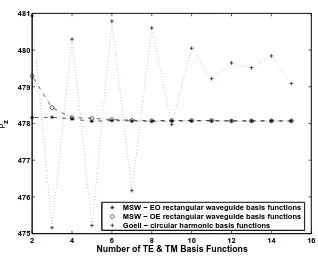
4.10 Comparison of the convergence properties of the Goell and MSW meth-ods when used with a square cross-section dielectric rod waveguide (εr2 =
37.4) in free-space. The propagation coefficients of the degenerate modes
Ex
11 and E11y are calculated using EO and OE symmetry respectively. . . 83
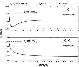
4.11 Effect of the proximity of the shield on βz, εr2 = 37.4, a1 = b1=6mm,
frequency=3.5GHz. . . 84
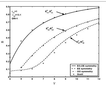
4.12 Comparison of theβzcalculation methods of MSW and Goell for a square
cross-section dielectric rod waveguide in free-space, where B and V are the normalised propagation coefficient and frequency respectively (εr2 =
13.1). . . 85
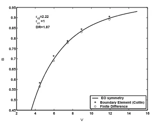
4.13 Comparison of the βz calculation methods of MSW, the boundary
el-ement method of Collin and the finite difference method of Schweig and Bridges for a shielded square cross-section dielectric rod waveguide,
SDDR= 1.87, εr2 = 2.22, where B and V are the normalised
propaga-tion coefficient and frequency respectively. . . 86
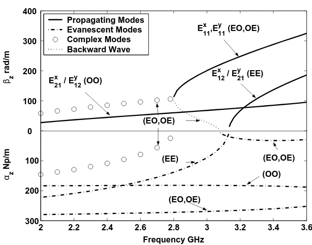
4.14 Mode diagram for the first few modes to propagate in a shielded dielec-tric rod waveguide plus some of the associated complex modes, evanes-cent modes and backward waves. DDR = 1(a1=6mm), SDDR =
2(a2=12mm),εr2 = 37.13. The modes are labeled with their associated
symmetry in parentheses. . . 87
4.15 Plot of the electric and magnetic fields (εr2 = 37.13) of the E11x mode
from the MSW method and EO symmetry. Quarter of the structure. . . 89
4.16 Plot of the electric and magnetic fields (εr2 = 37.13) of the E11y mode
from the MSW method and OE symmetry. Quarter of the structure. . . 89
4.17 Plot of the electric and magnetic fields of the coupledEx
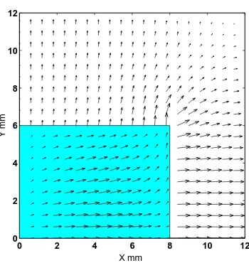
21andE12y modes
with dielectric aspect ratio DDR = 1, OO symmetry. NB electric field intensity in the dielectric x 5. Quarter of the structure. . . 89
4.18 Plot of the electric field (εr2 = 37.13) of the E21x mode with dielectric
aspect ratio DDR = 1.33 (E12y now non propagating), OO symmetry. NB electric field intensity in the dielectric x 10. Quarter of the structure. 90
structure. . . 90
4.20 Setup for an S11 measurement of the shielded dielectric waveguide. . . . 91
4.21 Calculated propagation coefficient values for the first few modes to prop-agate, shield-to-dielectric dimension ratioSDDR= 1.5. The modes are labeled with their associated symmetry in parentheses. . . 93
4.22 S11 Magnitude Data for the frequency range 2.0 to 3.6 GHz . . . 93
4.23 Comparison ofβz(N) propagation coefficients, at the measured resonant
frequencies, and calculated propagation coefficients for the Ex11 or E11y
mode. . . 94
4.24 Comparison ofβz(N) propagation coefficients, at the measured resonant frequencies, and calculated propagation coefficients for theEx
21/E
y
12
cou-pled mode. . . 94
4.25 A root of a transcendental equation close to a singularity. This wavenum-ber can be missed by a root finding function if the estimate step size is too high. . . 96
4.26 Convergence properties of rectangular shielded dielectric rod resonator for different shield-to-dielectric dimension ratiosSDDRsand a compari-son with the propagation coefficients corresponding to measured recompari-sonant frequencies. . . 97
4.27 Normalised intensities of the electric field components at the mode match-ing boundary. RegionII1/II2is compared to regionI. N = 8,SDDR=
2,a1 =b1= 6mm, a2 =b2 = 12mm . . . 99
4.28 Normalised intensities of the magnetic field components at the mode matching boundary. Region II1/II2 is compared to region I. N = 8,
SDDR= 2,a1 =b1 = 6mm, a2=b2= 12mm . . . 99
4.29 Normalised intensities of the electric field components at the mode match-ing boundary. Region II1/II2 is compared to region I. N = 11,
SDDR= 2,a1 =b1 = 6mm, a2=b2= 12mm . . . 100
4.30 Normalised intensities of the magnetic field components at the mode matching boundary. Region II1/II2 is compared to region I. N = 11,
SDDR= 2,a1 =b1 = 6mm, a2=b2= 12mm . . . 100
5.1 Shielded dielectric rod waveguide . . . 104
5.2 One quadrant of the cross-section, showing mode matching regions . . . 105
5.3 One quadrant of the cross-section, showing grid for power loss calcula-tion. . . 108
of the absolute value of the determinate. The mode is E11 from EO symmetry, a1 = b1 = 6.025mm, the shield-to-dielectric dimension ratio
SDDR=a2/a1 = 2, Frequency =3.4GHz,βz lossless=288.2 rad/m. . . 111
5.5 Attenuation coefficient versus frequency for the E11y mode. The shield-to-dielectric dimension ratio SDDR=a2/a1 = 2. . . 113
5.6 Attenuation coefficient versus frequency for the E21x/E12y coupled mode. The shield-to-dielectric dimension ratio SDDR=a2/a1 = 2. . . 113
5.7 Attenuation coefficient versus dielectric to shield dimension ratio for the
E11y mode. The frequency is 3.4GHz. . . 114 5.8 Attenuation coefficient versus dielectric to shield dimension ratio for the
coupled E21x/E12y . The frequency is 3.4GHz. . . 114 5.9 Electric and magnetic field patterns in the x-y plane for theE11y mode
for quarter of the structure. . . 116
5.10 Electric and magnetic field patterns in the x-y plane for the coupled
Ex
21/E
y
12 modes for quarter of the structure. . . 117
5.11 Extrapolation of the grid method, wall and dielectric loss values to
SDDR = 1. Comparison is made with those calculated for the T E10
mode in dielectric filled rectangular waveguide using an analytical method.119
5.12 Extrapolation of the grid method, wall and dielectric loss values to
SDDR = 1. Comparison is made with those calculated for the T M11
mode in dielectric filled rectangular waveguide using an analytical method.119
5.13 Set up of the dielectric resonator used for the measurement of unloaded Q. . . 121
5.14 Calculated and measured propagation coefficient values for the first few modes to propagate, shield-to-dielectric dimension ratio SDDR= 1.49. 125
5.15 Calculated and measured propagation coefficient values for the first few modes to propagate, shield-to-dielectric dimension ratio SDDR= 1.98. 125
5.16 Calculated and measured Q factor of the E11y mode for the 85mm long, WR159 shielded, square cross-section dielectric rod resonator. Dimen-sions: a1 =b1 = 6.025mm, a2 = 20.1mm,b2 = 10.045mm. . . 127
5.17 Break up of the calculated Q factor components of the E11y mode for 85mm long, WR159 shielded, square cross-section dielectric rod res-onator. The upper graph shows all the Q components due to dielectric loss Qd, end plate loss Qe and shield wall loss Qw. The lower magnified
graph shows Qd and Qe only. Dimensions: a1 = b1 = 6.025mm, a2 =
20.1mm,b2 = 10.045mm. . . 127
1 1 2 2
5.19 Flow chart of the program to find the attenuation due to power losses of the shielded rectangular dielectric rod waveguide and the Q factor of the test resonator. . . 130
A.1 Single coaxial resonator coordinate system and designations applicable to the equations presented in this appendix . . . 153
B.1 One quarter of the rectangular dielectric line with shield, showing mode-matching regions and designations applicable to the equations presented in this appendix. . . 157
C.1 Typical lightly coupled reflection coefficient response data (N = 2) from the WR159 shielded dielectric resonator of Chapter 5. . . 168
C.2 A least squares fit circle to the N = 2, Ey11, mode reflection coefficient response data from the WR159 shielded dielectric resonator of Chapter 5. . . 169
C.3 Close up of a least squares fit circle to the N = 2, E11y mode, reflection coefficient response data from the WR159 shielded dielectric resonator of Chapter 5. . . 169
C.4 Close up of a least squares fit circle to the N = 2, E11y mode, reflection coefficient response data from the WR159 shielded dielectric resonator of Chapter 5. Off resonance points removed . . . 170
C.5 Least squares fit line to the, N=2, Ey11 mode, reflection coefficient re-sponse data from the WR159 shielded dielectric resonator of Chapter 5. Off resonance points removed. . . 171
Introduction
1.1
Project Background
An increasing requirement of mobile phone technology is to fit as many radio frequency channels as possible into the available frequency spectrum. This is not only to make efficient use of the bandwidth, it also reduces congestion for users and increases the revenue available to mobile phone companies. Another aspect of the mobile system is that, during a call, the transmitter and receiver at each end must both be on so that the users of a phone connection can converse at the same time. To achieve sufficient signal selectivity and rejection, stringent specifications are required for the dielectric loaded cavity filters employed in the mobile phone base stations. In the context of base station filters, the limit of present technology is multimode filter design.
Multimode filters are made up of coupled resonant cavities each containing a cylindri-cal or rectangular block of ceramic material having a high dielectric constant. These dielectric resonators store most of the electromagnetic energy and the cavity walls sur-rounding them are principally there to provide shielding. The dielectric resonators also allow smaller cavity size and lower energy loss compared to non-dielectric filters. This allows a sharper filter response and greater unwanted signal rejection. The term
multimode can be explained with reference to a dual-mode waveguide filter where n
series cavities each support two orthogonally polarised degenerate mode resonances. Applying this technique a 2nth degree filter can be constructed with n cavities giving a significant reduction in size compared to a conventional filter, in which each cavity supports only one resonant mode (Hunter, 2001, p. 255).
Due to difficulties caused by the interaction between components, a lot of design work on filters is still performed empirically, as in the case of the coupled dielectric resonator filter described by Walker & Hunter (2002). This is because a complete knowledge of the electromagnetic fields in the coupled cavity sections has not been achieved (Rong & Zaki, 1999). Because of their increased complexity this is especially true for the multimode dielectric loaded cavity filters.
At present commercial software packages using Finite Element (FEM) or Finite Differ-ence Time Domain (FDTD) methods are used to overcome this. These methods work well but processing a solution of sufficient accuracy requires a large number of points or elements (large memory requirement) and can be very time consuming. If a structure is doubled in size in all coordinate directions (ie grid cell numbers increased by 23), or
equivalently if the frequency is doubled, a 3-D FEM solution could take up to 64-times as long (depending on the sparsity of the matrix and how well the FEM software can use this to advantage) , or 16 times for a FDTD solution (Veidt, 1998, p. 134). Rong & Zaki (1999) have stated that the standard of efficiency of general purpose numerical methods using FEM (example given: Hewlett Packard HFSS) makes their use for filter design impractical.
in that it allows an analytical analysis of the solution once the unknown coefficients are found. This provides an insight into the mode structure which would be difficult to achieve using purely numerical methods. For example, the results for shielded dielectric rod waveguide show that this structure is capable of supporting complex modes and backward waves, in addition to the expected propagating and evanescent modes.
During discussions with Brisbane based filter manufacturer Filtronic1, the use of the
mode matching method was proposed to remedy some of the commercial solver prob-lems as well as to predict interactions between coupled multimode resonant cavities. Although a lot of work has been done in this area over the past 10 years, no com-mercial software package is available that can solve the present problems in multimode dielectric loaded filter design.
This being the case, and as investigations into the use of cubic dielectric loaded res-onators were being carried out by Filtronic and others, an improved theoretical under-standing of these structures was desirable; and the MM technique provided a means to achieve this. Specifically, the study of the shielded rectangular dielectric rod waveguide could be seen as a basic precursor to the analysis of the cubic dielectric loaded cavity resonator. The latter procedure would take a similar path to that of Zaki & Atia (1983) where a cylindrical dielectric rod enclosed in a cylindrical waveguide was modeled and the propagation coefficients of the fundamental modes were found. Metallic plates were then placed on the ends of a section of this waveguide forming a cylindrical dielectric loaded cavity resonator. Mode matching was then used to solve the resonant frequency eigenvalue problem. Later Liang & Zaki (1993) extended this to cylindrical dielectric resonators in rectangular waveguide and cavities.
1.2
The Proposition of the Thesis
The proposition of this thesis is that the mode matching method has significant ad-vantages for the analysis of the electromagnetic fields of structures used in current dielectric loaded multimode cavity filters. In general the method requires less CPU time than a strictly numerical procedure, such as the finite element method, due to its inherent analytic pre-processing; and it also provides a better physical understanding of the field structure.
1.3
Aim and Objectives
The broad aim of the project is to perform electromagnetic field analysis on the shielded rectangular dielectric rod waveguide using the mode matching method.
The specific objectives of the project are as follows:
1. (a) To perform a literature survey on the use of mode matching in general and to replicate the results of some of the early work associated with rectangular waveguide discontinuities. A number of computer programs would have to written to achieve this and would provide confidence in the validity of later original work.
(b) Apply mode matching to the analysis of cylindrical structures such as a coaxial resonator. This work was seen as an exercise in the use of mode matching to solve eigenvalue problems. For the case of the coaxial resonator these values are the resonant frequencies of the structure. In the event this work produced some original results suitable for publication it would be included in the thesis.
and of the losses associated with this structure. This would provide a foundation for a complete analysis of shielded rectangular cross-section dielectric resonators (as has been achieved for cylindrical resonators (Zaki & Atia, 1983)).
1.4
Overview of the Thesis
Chapter 1
Introduction
Chapter 1 introduces the proposition driving this research, namely that the mode matching method has some advantages for the electromagnetic analysis on a struc-ture associated with the latest dielectric loaded multimode cavity filters. Chapter 1 also outlines the aim and objectives of the research and highlights those areas where original work has been performed.
Chapter 2
Overview of the Mode Matching Method
The first part of Chapter 2 presents two literature surveys, firstly to give some back-ground to the project in the area of microwave cavity filters and secondly the theory and application of mode matching techniques. The second part of Chapter 2 details mode matching theory related to rectangular waveguide discontinuity problems. The last part of the chapter gives an insight into some of the early work accomplished in applying the mode matching procedure. This is shown by comparing some of the re-sults from literature for waveguide discontinuity problems with those from computer programs written to replicate them.
Chapter 3
The Coaxial Resonator
rod (single coaxial resonator) is studied. A simplified mode matching procedure is used to find the TEM mode resonant frequencies and gap capacitance. This chapter is an expansion of a paper published in IEE Proceedings on Microwave Antennas and Propagation (Wells & Ball, 2004).
Chapter 4
The Shielded Rectangular Dielectric Rod Waveguide
In Chapter 4 the mode matching method is developed to allow the computation of the propagation coefficients and field patterns of the fundamental modes in a shielded rectangular dielectric rod waveguide. The full solution described in this chapter shows the results of all the dominant modes and field patterns. It also shows that in addition to conventional waveguide modes the structure can support complex waves and backward waves. This original work is an expansion of a paper published inIEEE Transactions on Microwave Theory and Techniques (Wells & Ball, 2005b).
Chapter 5
Attenuation of a Shielded Rectangular Dielectric Rod Waveguide
In this chapter the calculated fields, found using the mode matching method of Chapter 4, are employed to find the wall and dielectric losses of the waveguide and hence its attenuation. For theEy11 mode and the dominant Ex
21/Ey12 coupled mode the effect of
the proximity of the shield on the attenuation is also be evaluated. This work is original, and is an expansion of a paper submitted for publication (Wells & Ball, 2005a).
Chapter 6
Conclusion
This chapter summarises the major findings of the thesis and their significance to the wider body of knowledge in the field. The chapter concludes with a summary of suggested areas for future work.
Coaxial Resonator Mode Matching Equations
This appendix provides a summary of the basis functions and integrals used in the mode matching method developed for the coaxial resonator in Chapter 3.
Appendix B
Shielded Rectangular Dielectric Rod Mode Matching Equations
This appendix provides a summary of the basis functions, continuity equations at boundaries and integrals used in the mode matching method developed for the shielded rectangular waveguide in Chapter 4.
Appendix C
Calculation of Unloaded Q Factor from the Measured Reflection Coefficient
of a Resonator
In this appendix the method used for determining unloaded Q factor from the measured reflection coefficient S11 of the resonant structures of section 5.6 is described.
Appendix D
Guide to the Thesis Companion Disk
This appendix provides a guide to the thesis companion disk. The disk contains a copy of the dissertation and a basic cross-section of the main computer programs for the coaxial resonator of Chapter 3, the rectangular shielded dielectric rod of Chapter 4 and for the rectangular shielded dielectric rod attenuation in Chapter 5.
1.5
Summary of Original Work
The areas of this project where original work has been performed are summarised below.
resonator, and calculation of the gap capacitance.
2. Calculation of the propagation coefficients of the modes in a shielded rectangular dielectric rod waveguide. Propagating, complex, evanescent and backward wave modes were included and the work showed the presence of a dominant mode, and other fundamental modes, not previously identified. The effect of the proximity of the shield to the dielectric rod on the propagation coefficient and mode structure was also investigated.
3. Calculation of the attenuation coefficient of the commonly used E11y mode, and other fundamental modes, in a shielded rectangular dielectric rod waveguide. The influence on the attenuation coefficient of the proximity of the shield to the rod was also evaluated.
1.6
Publications
Wells, C. G. & Ball, J. A. R. (2004), ‘Gap capacitance of a coaxial resonator using simplified mode matching’,IEE Proceedings on Microwave Antennas and Propagation,
151(5), 399 -403.
Wells, C. G. & Ball, J. A. R. (2005), ‘Mode matching analysis of a shielded rectangu-lar dielectric rod waveguide ’,IEEE Transactions on Microwave Theory and Techniques,
53(10), 3169-3177, October.
Overview of the Mode Matching
Method
2.1
Introduction
This chapter begins with a description of two literature surveys. The first is on the topic of microwave cavity filters. This describes how these filters have evolved from simple cavity and combline filters of forty years ago to the small multimode dielectrically loaded high selectivity types of today. The second describes how the mode matching method has been used over this same period to solve at first, waveguide discontinuity problems, and then later, aid in the design of combline, finlines, microstrip lines and many other structures including dielectric loaded cavity filters.
Section 2.4 details the basic theory behind the mode matching method. The problem of the junction of two rectangular waveguides in a boundary reduction configuration is used as an example.
Finally section 2.5 describes the results obtained from a mode matching program writ-ten for the rectangular waveguide discontinuity problem of the previous section. This
program was written to gain experience in writing mode matching code, by using past papers as a procedural guide (no code is ever given), and comparing the results with those published.
2.2
Microwave Cavity Filters
A generation ago virtually all design information available on microwave filters was summarised in the classic text titled “Microwave Filters, Impedance Matching Networks and Coupling Structures” (Matthaei et al., 1984). Amongst other types, this dealt with design of combline filters, from which present day base station filters could be said to have evolved.
In the early 1970s dual mode filters, which effectively double the use of a cavity and make the overall filter smaller, were introduced by Atia & Williams (1972). An other step forward occurred when Fiedziuszko (1982) described dual mode dielectric loaded filters. These allowed further size reduction, improved in-band performance and pro-vided greater thermal stability. Wang et al. (1998) described a dielectric loaded version of the combline filter which combined the merits of the metallic combline and dielectric loaded filters. A mode matching method was used to model the electromagnetic fields in the filter from which filter parameters were calculated. Sabbagh et al. (2001) and Wu et al. (2002) then described methods for solving problems in this type of filter when a number of interacting combinations of resonant cavities in the same type of filter were coupled together.
2.3
Brief History of Mode Matching Method
in Filter Design
and other numerical methods, have been devised and then gradually improved to cope with the invention of many new and complex microwave structures. Initially, these were applied to the analysis of the discontinuities in rectangular waveguides.
The use of computer-aided mode matching to calculate the fields of simple structures began in the 1960s with papers by Wexler (1967) and Clarricotes & Slinn (1967). The use of computers has been an essential part of the method’s development because of the amount of repetitive calculations required to reach a solution.
Luebbers & Munk (1973) used the method to calculate the reflection and transmission properties of a thick rectangular window in centrally located in a rectangular waveguide. The waveguides on either side of the window had to be identical.
Patzelt & Arndt (1982) and Safavi-Naini & Macphie (1982) adapted the method to solve problems involving the junction of rectangular to rectangular waveguide steps as used in waveguide transformers, irises (small windows across the waveguide) and reactance coupled filters. By addition of the use of a technique involving the conservation of complex power, rapid convergence of numerical results was achieved (Safavi-Naini & Macphie, 1981). Also the results of a junction were presented in the form of a scattering (S) parameter matrix. This enabled a number of cascaded junctions in a system to be analysed in a unified manner.
Omar & Schunemann (1985) showed that the orthogonality relations associated with the cross-product of field vectors, as used sometimes in mode matching, were again related to the conservation of complex power 1 and hence good convergence properties could be obtained. Also transmission matrix results were used in the formulation of a multi-section finline bandpass filter. Calculations with this type of matrix have lower computation time than with the S parameter matrix, but problems can sometimes occur with the convergence of a solution (Alessandri et al., 1988).
1Complex power is the combination of the real and reactive power of the electric and magnetic fields
About the same time Chu & Itoh (1986) modeled cascaded microstrip step disconti-nuities using mode matching. An equivalent waveguide model was introduced for the microstrip line. Also Wade & Macphie (1986) used the method to determine exact solutions at the junction of circular and rectangular waveguide. James (1987) provided solutions to irises in coaxial and circular waveguides.
Analyses of dielectric inserts in waveguide first appeared in 1988 (Gesche & Lochel, 1988), (Zaki et al., 1988). Also a more formalised approach to the cascading of junc-tion discontinuities in general were formulated in a paper by Alessandri et al. (1988). Particular types of junction problems were recognised and placed into so called mode matching building blocks allowing the Computer Assisted Design (CAD) of a large class of waveguide components (Arndt et al., 1997). It may be possible to use a variation of this approach to analyse microwave filters.
A number of papers, spanning the early 1990’s and extending this formalised approach, then appeared for rectangular waveguide: Sieverding & Arndt (1992) for the T-junction building block and Reiter & Arndt (1992) for cascaded H-plane discontinuities.
2.4
Mode Matching
The mode matching procedure is useful for solving scattering parameter problems at a discontinuity in a structure. It can be applied to junctions of different types of waveg-uide or posts or obstructions in a wavegwaveg-uide. Additionally it can be used in eigenvalue problems such as finding the resonant frequency of a cavity, the cutoff frequency of a waveguide or the propagation coefficient of a transmission line.
2.4.1 Basic Procedure
To model a discontinuity a structure is divided into separate regions either side of the discontinuity. The fields in each region are expressed as a sum of modes. In the case of common rectangular waveguide these modes would be the electric and magnetic TE and TM modes of homogeneously filled rectangular waveguide. By matching the tangential components of the modes at the boundary between regions and using their orthogonality properties an infinite set of linear equations can be obtained.
A number of formulations are available in the literature to achieve this, and the principal difference between these lies in the method they use to expand the mode functions to form an infinite set of equations. The method of Shih, described in Itoh (1989), uses the dot product of testing functions with the mode functions whereas the method described by Eleftheriades et al. (1994) uses a cross product. Ultimately there does not appear to be a significant difference in the results using either of these methods and the final decision of which to use comes down to the ease by which they can be applied to the type of structure involved.
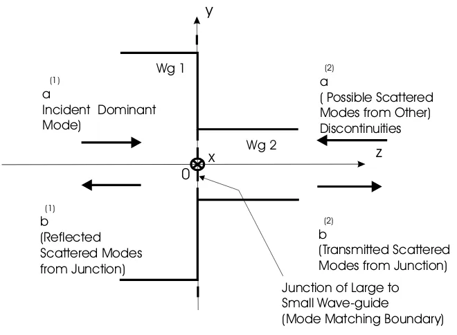
Wave-guide 2
Wave-guide 1 S2 Cross-sectional
Area W/G 2 S1 Cross-sectional
Area W/G 1
Figure 2.1: Boundary Reduction Wave-guide Configuration
Scattering Matrix (GSM) from which the the scattering parameters of the discontinuity can be obtained.
2.4.2 A Boundary Reduction Discontinuity Problem
The mode matching technique is usefully illustrated by means of a simple example, that of the determination of the scattering parameters of a waveguide discontinuity.
a
Incident Dominant Mode)
(1)
(1) b
(Reflected Scattered Modes from Junction)
(2) b
(Transmitted Scattered Modes from Junction)
Junction of Large to Small Wave-guide
(Mode Matching Boundary) (2)
a
( Possible Scattered Modes from Other) Discontinuities
0
z y
x Wg 1
[image:33.595.157.487.102.344.2]Wg 2
Figure 2.2: Forward and Reflected Components at a BR Wave-guide Junction
together by the algebraic combination of their S matrices. Figure 2.2 shows how the forward (a(1),a(2)) and the reflected (b(1),b(2)) modal amplitude vectors are arranged at the junction.
To implement the mode matching procedure the tangential components of the modes are forced to be continuous at the mode matching boundary. The boundary conditions to be satisfied are:
E(1)t =
E(2)t onS2
0 onS1−S2
(2.1)
H(1)t = H(2)t onS2 (2.2)
where
S1 and S2 are the cross-sectional areas of waveguides 1 and 2 respectively; and
E(1)t =
∞
X
m=1
(a(1)m e−γ1z+b(1) m eγ1z)e
(1)
tm (2.3)
E(2)t =
∞
X
n=1
(b(2)n e−γ2z+a(2) n eγ2z)e
(2)
tn (2.4)
H(1)t =
∞
X
m=1
(a(1)m e−γ1z−b(1) m eγ1z)h
(1)
tm (2.5)
H(2)t =
∞
X
n=1
(b(2)n e−γ2z−a(2)
n eγ2z)h(2)tn (2.6)
wherem and nare all the TE and TM modes of rectangular waveguide in waveguides 1 and 2 respectively and aandb are the amplitude coefficients of those modes.
The transverse components (at the z = 0 boundary) can be written from those in Pozar (1998) as:
e(xip q) =
−qA(i) B(i) pBA((ii))
cosβxpxsinβyqy T E T M (2.7)
e(yip q) = p q
sinβxpxcosβyqy T E T M (2.8)
h(xip q) =
−pYh ω
−qYωe
sinβxpxcosβyqy T E T M (2.9)
h(yip q) =
−pBA((ii))Yωh qB(i)
A(i)Yωe
cosβxpxsinβyqy T E T M (2.10) where
β2xp+βy2q =γp q2 +β02εr (2.11) Yωh = γp q
ωµ0
; Yωe= ωε0εr
γp q
(2.12)
βxp =
pπ
A(i); βyq =
qπ B(i); β
2
0 =ω2µ0ε0 (2.13)
and A(i)and B(i) are the width and height of the waveguides respectively and p and q
To implement the mode matching procedure on a computer it is necessary to truncate the infinite number of modes involved to a value that will give the required accuracy in the solution. Increasing numbers of modes are tried in the initial computation until the result converges to a sufficiently constant value. The maximum number of modes allocated for computation in waveguides 1 and 2 will now be designated M and N
respectively.
For proper convergence of the solution the number of modes in the larger waveguide should always be greater than that in the smaller, ieM > N for Figure 2.2. If this is not done there could be a violation of the field distributions at the edge of a conductive boundary and ill-conditioning of the linear system of equations themselves can also occur (Mittra & Lee, 1971). This is a consequence of truncating the number of modes in each region from their true infinite value and in calculation is equivalent to truncating two infinite series (Itoh, 1989, pp. 603-4). It will be shown later in section 2.5 that the numerical solution will converge to different values depending on the ratio of the number of modes chosen in each region. This phenomenon is called relative convergence and is a limitation to the accuracy of the mode matching procedure. Fortunately some simple rules can be employed to minimise its effect on accuracy. For example, for a boundary reduction in height only, researchers have found that keeping the ratio of modes in each waveguide region equal to that of the ratio of corresponding regional cross-section side lengths gives optimum results (Itoh, 1989, p. 613).
& Schunemann, 1985) and also allows a better understanding of the mode matching method and makes it easier to write a workable program. This procedure is as follows:
1. Find the cross product of the electric field equations on both sides of the junction with a testing function from the magnetic field equation of the waveguide 1 and integrate.
In wave-guide (1)
Z
s1
em(1)×h(1)n ·z dsˆ =Pm(1)δmn (2.14)
In wave-guide (2)
Anm=
Z
s2
e(2)m ×h(1)n ·z dsˆ (2.15)
2. Find the cross product of the magnetic field of waveguide 2 with a testing func-tion from the electric field equafunc-tion of the same waveguide and integrate, ie
Z
s2
en(2)×h(2)m ·z dsˆ =Q(2)n δnm (2.16)
Note that the integral of the cross product of the magnetic field of waveguide 1 with a testing function from the electric field equation of waveguide 2 could be calculated as:
Bmn=
Z
s2
e(2)m ×h(1)n ·z dsˆ (2.17) However, in view of the equality:
Bmn=Atnm (2.18)
where superscripttmeans transpose, only Anm need be calculated.
In equations (2.14), (2.15), (2.16) and (2.17)mandnare the TE plus TM modes used where:
m = 1,2, ..., M
n = 1,2, ..., N (2.19)
3. The amplitude vectors can then be related by two sets of linear equations in matrix form:
[λP] ( [a(1)] + [b(1)] ) = [Anm] ( [a(2)] + [b(2)] ) electric field (2.20)
[Anm]t( [a(1)]−[b(1)] ) = [λQ] ( [b(2)]−[a(2)] ) magnetic field (2.21)
where:
λP = (Pm(1)δmn) andλQ= (Q(2)n δnm) are diagonal matrices of M xM andN xN
respectively. They contain the normalisation constants for each individual mode in each wave-guide and:
Anm and Atnm are N x M and M x N matrices respectively which show the
reaction or coupling between modes across the wave-guide junction.
From these sets of linear equations the unknown coefficients (a(1),a(2),b(1) andb(2)) of the BR junction can be found or the Generalised Scattering Matrix (GSM) can be derived:
1. In the method described by Wexler (1967) the electric field equation was re-arranged for theb(1) coefficients and the resultant equation was substituted into the magnetic field equation to eliminate them. This, and the fact that the a(1)
modal input and the scattered modes from a later junctiona(2) would be known, gave sufficient equations to solve for the b(2) coefficients. These could then be substituted into the original equations to find the remaining b(1) coefficients.
2. In the method described by Omar & Schunemann (1985) the GSM for the junction is derived. Firstly the equations are arranged into the following form:
a(1)+b(1) = [R]·(a(2)+b(2)) (2.22)
[T]·(a(1)−b(1)) =b(2)−a(2) (2.23) where:
and
[T] = [λQ]−1·[Anm]t
By dividing these equations through by the appropriatea(j)coefficient calculation of the S matrix elements can be performed by use of the standard formula:
Sij= b
(i)
a(j)
ak=0f or k6=j
(2.24)
Using this procedure Omar & Schunemann (1985) give the S parameters, which are actually GSM parameters, as:
[S11] = ([R][T] + [I])−1·([R][T]−[I]) (2.25)
[S12] = 2([R][T] + [I])−1·[R] (2.26)
[S21] = [T]([I]−[S11]) (2.27)
[S22] = [I]−[T][S12] (2.28)
where:
I is the identity matrix.
The scattering matrix representation can then be written as:
b(1) b(2)
=
[S11] [S12]
[S21] [S22]
·
a(1) a(2)
(2.29)
2.5
Numerical Results for the Boundary
Reduction Discontinuity
A computer program was written to duplicate a number of the results found in literature for this type of discontinuity. This was done so as to gain experience in producing mode matching code and also to be able to experiment with some of the problems associated with the method such as relative convergence (see section 2.4.2).
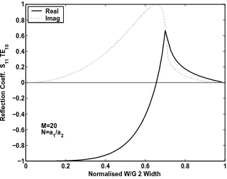
0 0.2 0.4 0.6 0.8 1 −1
−0.8 −0.6 −0.4 −0.2 0 0.2 0.4 0.6 0.8 1
Normalised W/G 2 Width
Reflection Coeff. S
11
TE
10
Real Imag
M=20 N=a
[image:39.595.160.480.108.361.2]1/a2
Figure 2.3: Reflection coefficientS11of the incidentT E10mode to the BR
discon-tinuity
range of the larger and the reflection coefficientS11of an incidentT E10mode was found
to be as in Figure 2.3. For calculation the larger waveguide (1) dimensions were made the same as WR284 (72.14 x 34.04mm) and the frequency was determined from the free space wavelengthλ, calculated as:
λ= a1
0.71 (2.30)
wherea1is the width of the large waveguide. This is the same as that used in a paper by
Shih & Gray (1983) referred to later. TwentyT Ep0 modes (M) were used in waveguide
(2) and N modes in waveguide 1 calculated from the expression:
N =Ma1 a2
(2.31)
Wherea1 and a2 are the widths of waveguides 1 and 2 respectively.
This is to satisfy the relative convergence criteria.
When a T E10 mode is incident on this type of structure only the T Ep0 modes are
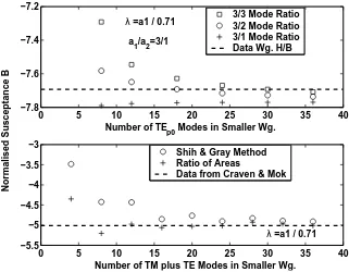
0 5 10 15 20 25 30 35 40 −7.8
−7.6 −7.4 −7.2
Normalised Susceptance B
Number of TE
p0 Modes in Smaller Wg.
3/3 Mode Ratio 3/2 Mode Ratio 3/1 Mode Ratio Data Wg. H/B
0 5 10 15 20 25 30 35 40
−5.5 −5 −4.5 −4 −3.5 −3
Number of TM plus TE Modes in Smaller Wg. Shih & Gray Method Ratio of Areas
Data from Craven & Mok
λ =a1 / 0.71 λ =a1 / 0.71
a
[image:40.595.159.480.108.358.2]1/a2=3/1
Figure 2.4: Mode matching susceptance results for the change in cross-section of a rectangular waveguide. Upper graph: symmetrical change in width only (single step) with a waveguide region width ratio of 3/1. Lower graph: symmetrical change in height and width (double step) with a waveguide region height and width ratios of 2/1.
approached as the width of waveguide 2 draws near to zero and the reflection becomes minimal as the width of the waveguides become the same.
An investigation into the input susceptance results using mode matching for a BR junction was described in a paper by Shih & Gray (1983). In this paper both the single step (width only case of the previous example in this section) and also a double step, where both the height and width are varied symmetrically, are described. This procedure was duplicated using the program written and the results are shown in Figure 2.4. The the upper graph shows the convergence characteristics for the single step with a waveguide region height ratio a1/a2 = 3/1 compared to a number of mode ratios.
0.9 1 1.1 1.2
x 1010
0 0.5 1 1.5
Frequency Hz
Magnitude S
11
0.9 1 1.1 1.2
x 1010
0 50 100 150
Frequency Hz
Phase S
11
deg
0.9 1 1.1 1.2
x 1010
1.5 2 2.5 3 3.5 4
Frequency Hz
Magnitude S
21
0.9 1 1.1 1.2
x 1010
0 20 40 60 80
Frequency Hz
Phase S
21
deg
Figure 2.5: Duplication of the results of Figure 3 Safavi-Naini & McPhie (1982). Magnitude and phase ofS11 andS21 for the BR junction double step.
The ratio of areas and the Shin and Gray method (Shih & Gray, 1983) give similar convergence.
For a higher number of modes, where convergence is best, the calculated results compare well with those from the Waveguide Handbook (Marcuvitz, 1951) for the single step (within 1% for 36 modes in the input waveguide). Similarly for the double step the calculated results are within 2% or less of the approximation of Craven & Mok (1971) for 36 input waveguide modes.
Finally the results for the double step BR junction from a paper by Safavi-Naini & Macphie (1982) were duplicated. The magnitude and phase of the reflection coefficient and the transmission coefficient from the calculated results are plotted in Figure 2.5 and are almost identical with the actual Safavi-Naini & Macphie (1982) results shown in Figure 2.6.
2.6
Conclusion
This chapter began with two literature surveys that gave a brief history of microwave cavity filters and the use of the mode matching method over the last forty years.
The basic theory behind the mode matching method was then described. To illustrate this a boundary reduction discontinuity problem in rectangular waveguide was used as an example.
Results from experiments using a mode matching program, written as an exercise to solve problems for this type discontinuity, gave information on the nature of the rate of convergence and the relative convergence problem. These problems were found to be associated with the number of modes and the ratio of the number of modes in each region.
The Coaxial Resonator
3.1
Introduction
After the initial introduction to mode matching through the analysis of rectangular waveguide discontinuities, the coaxial resonator was selected as it was considered that this would be a good learning exercise in using the method with regard to resonators and the inherent eigenvalue problem of finding the resonant frequency.
Coaxial filters are used in wireless and mobile communication applications due to their small size, low cost and relatively high Q factor. Traditionally these filters have been designed using filter theory based on TEM mode transmission line structures (Matthaei et al., 1984).
In this chapter a coaxial line in the form of a cylindrical cavity with a centre conductive rod (single coaxial resonator) as shown in Figure 3.1 will be studied. A simplified mode matching procedure is used to find the TEM mode resonant frequencies. This chapter is an expansion of a paper published inIEE Proceedings on Microwave Antennas and Propagation (Wells & Ball, 2004).
The coaxial line studied is less than λ4 in length, with open and short circuit ends.
The inductance provided by the line at the open circuit, and capacitance due to the gap Cg, provide conditions for a resonant circuit. The resonant frequency can be adjusted by altering the gap capacitance with the aid of a tuning screw. Size constraints may require the coaxial line length to be reduced to λ8 or less, which means that a substantial capacitance is required to bring the structure to resonance. This in turn means the gap must be quite small. However calculation using a parallel plate capacitance model will only give an approximate resonant frequency for the structure, as the total capacitance will be larger due to fringing effects around the open circuit end of the centre conductor. If a tuning screw is added, as shown in the figure, it will further complicate the capacitance evaluation.
Inner Conductor
Outer Conductor Gap Capacitance Cg Short Circuit Open Circuit
Tuning Screw
Figure 3.1: Single Coaxial Transmission Line Resonator
This problem can be overcome by the use of a rigorous mode matching method (Wexler, 1967) (Omar & Schunemann, 1985) to compute the resonant frequency of the cavity, and hence the gap capacitance. The cavity is partitioned into two cylindrical regions, as in Figure 3.2, and the fields in each region are represented as linear combinations of radial basis functions1. Since only the lowest order quasi-TEM resonant frequency is required,
only radial basis functions having no circumferential variation need be included. The transverse fields are matched at the boundaries between regions to ensure that they are continuous, and a set of simultaneous equations is produced. The resonant frequency is found by equating the determinant of this system to zero. Resonant frequencies computed in this way show excellent agreement with measured results.
1To reduce confusion with the term ‘modes’, the modes of radial waveguide, used to ‘build up’ the
Once the resonant frequency has been found, the gap capacitance can be calculated. For filter applications, a requirement is to maximise the resonator Q-factor. This is accomplished by choosing the coaxial line radius ratio a/ro to be 3.591 (Sander, 1987, p. 24), which minimises the conductor losses in the coaxial surfaces. This corresponds to an air-spaced characteristic impedance of 76.7Ω. Values of gap capacitance are provided for this optimum situation.
I
II
Z
b
b
b
21
a
r
0Gap g=b -b2 1
Figure 3.2: Single Coaxial Resonator Coordinate System
3.2
Analysis using the Radial Mode Matching Method
so uses cylindrical waveguide basis functions. This method was not used as it requires the integral of the product of Bessel functions, which makes the problem more complex and increases the computation time (Chen, 1990).
The structure to be analysed is shown in Figure 3.2, and is composed of two air filled regions. Region I is the cylindrical gap between the inner rod and the tuning screw, assumed to be of the same diameter (b1 < z < b2, 0 < ρ < ro, 0 < φ < 2π). The
remainder of the cavity is region II (0 < z < b, ro < ρ < a, 0 < φ <2π). The mode
matching boundary is then defined as the surface: 0< z < b, ρ=ro, 0< φ <2π. All
metal surfaces will be considered to be perfect electric conductors (PEC). The fields within the structure are represented by superpositions of radial waves (basis functions), which propagate in the radial direction forming standing waves. Their form can be derived using the boundary conditions and the radial waveguide field equations as described by Balanis (1988). In this structure these equations can be greatly simplified by removing the circumferential variations. This can be justified by realising that for the radial basis functions to describe the field patterns of the TEM transmission line, only those parts describing the radial and longitudinal variations are necessary. This means that the TE basis functions can be neglected as there is noEz component, and
consulting the differential equations for the TE radial fields (Balanis, 1988, p. 501),Eρ
andHφ, which would be used to ‘build up’ a TEM mode, are zero as they are dependent
on φ. The general form of the magnetic vector potential in the structure would then be:
Az(ρ, φ, z) = (C1Ji(βρρ) +D1Yi(βρρ)) (C2sin (βzz) +D2cos (βzz))
·(C3sin (iφ) +D3cos (iφ)) (3.1)
and, using the simplification just described, the transverse magnetic (TM) radial basis function fields can then be derived from:
Az(ρ, φ, z) = (C1J0(βρρ) +D1Y0(βρρ)) (C2sin (βzz) +D2cos (βzz)) (3.2)
3.2.1 Radial TM Basis Functions
Region I
Using equation (3.2) and the appropriate boundaries, the magnetic vector potential field equation for the gap between the conductive rod and the tuning screw can be shown to be:
AzI(ρ, z) =A
T M
k J0(βρIρ) cos (βzI(z−b1)) (3.3) where:
βz =
kπ b2−b1
due to the top and bottom PEC boundaries at the rod and tuning screw ends.
The wave number in the radial direction βρ is related to βz, and to the wave number
of the mediumβ0, by the equations:
βρ2 =β02−βz2; β02 =ω2µ0ε0εr (3.4)
and the Bessel functions of the second kind (Y0) are infinite atρ = 0 and are therefore
not part of the solution.
The TM basis function component equations for region I are then found from the differential equations provided by Balanis (1988, p. 503). A summary of these are presented in Appendix A.
Region II
Ezwill be zero at the tangential outer cylindrical boundaryρ=a. This field component is related to the potential function by:
Ez =−j 1 ωµε
∂2
z2 +β 2
Az (3.5)
Using equations (3.2) and (3.5) and working backwards from the outer wall PEC bound-ary the potential function for region II must have the form:
AzII(ρ, z) =B
T M
n (Y0(βρIIa)J0(βρIIρ)−J0(βρIIa)Y0(βρIIρ)) cos(βzIIz) (3.6) where:
βzII =
nπ b
plates. The wave number in the radial directionβρII is related toβzII, and to the wave number of the mediumβ0, by the equations:
βρ2II =β02−βz2II; β02 =ω2µ0ε0εr (3.7)
The TM basis function component equations for region II are then found from the differential equations provided by Balanis (1988, p. 503). A summary of these are presented in Appendix A.
If the radial wave numberβρ is imaginary, then the basis function is non propagating,
and the fields will decay exponentially in the radial direction. This can occur in both regions, and with either basis function type. In this case the Bessel functionsJ0 andY0
for that particular basis function will have to be changed to modified Bessel functions
I0 andK0 respectively.
3.2.2 Mode Matching at the Boundary Between Regions
To find a field solution to the current problem the transverse (tangential) E and H fields in both regions must be matched at the cylindrical boundary ρ = ro. Each
field component is represented by a summation of radial basis functions. Matching the transverse electric fields across the boundary between regions I and II leads to:
E=AT Mp
∞
X
p=1
ET MI =BqT M
∞
X
q=1
ET MII (3.8)
where the TM basis function in region I is identified by p and the TM basis function in region II is identified byq.
Similarly, the transverse magnetic fields will be matched if the following condition holds:
H=AT Mp
∞
X
p=1
HT MI =BqT M
∞
X
q=1
HT MII (3.9)
orthogonality relation (inner product), as applied by Yao (1995), was used.
<Em,Hn>=
Z
S
(Em×Hn)·ds = 0 if m6=n (3.10)
This is applied to both equations (3.8) and (3.9). Firstly, form the cross-product of equation (3.8) and a testing function from the magnetic field of region II and integrate over the inner cylindrical surface of region II:
<E,hqII >=
b
Z
0 2π
Z
0
(E×hqII)·ρ rˆ odφdz (3.11)
For no circumferential variations this then becomes:
<E,hqII >=
b
Z
0
(E×hqII)·ρ dzˆ (3.12)
Secondly, form the cross-product of equation (3.9) and a TM testing function from the electric field of region I and integrate over the outer cylindrical surface of region I:
<epI,H>=
b2 Z
b1
2π
Z
0
(epI ×H)·ρ rˆ odφdz (3.13)
For no circumferential variations this then becomes:
<epI,H>=
b2 Z
b1
(epI ×H)·ρ dzˆ (3.14)
Therefore the testing functions required are only the z dependent factors of the basis functions.
The resultant equations in matrix form for the electric field are:
a11 . . . a1p
..
. . ..T ME(I)
zT M
(II)
hφ .. .
aq1 · · · aqp
AT M1
.. .
AT Mp
=
b11 · · · 0
..
. . ..T ME(II)
z T M
(II)
hφ .. .
0 · · · bqq
B1T M
.. .
BqT M
(3.15) or in an abbreviated form
[W][A] = [X][B] (3.16)
The magnetic field equations are:
a11 . . . 0
..
. . ..T MH(I)
φT M
(I)
ez ...
0 · · · app
AT M1
.. .
AT Mp
=
b11 · · · b1q
..
. . ..T MH(II)
φ T M
(I)
ez ...
bp1 · · · bpq
B1T M
.. .
BqT M
(3.17) and in abbreviated form
[Y][A] = [Z][B] (3.18)
The elements of [W] and [Y] are the result of the inner products on the LHS of equations (3.8) and (3.9) respectively, and those of [X] and [Z] are the results of the inner product on the RHS of the same equations. [X] and [Y] are diagonal matrices. [A] and [B] are the unknown coefficients. These equations can then be used to solve for the resonant frequencies of the structure or to find the unknown coefficients of the field equations.
3.2.3 Resonant Frequencies of the Structure
An efficient system of homogeneous equations may be formed from equations (3.16) and (3.18) by eliminating either the [A] or the [B] coefficients. It is preferable to eliminate [B], because this leads to a smaller matrix.
[Y]−1[Z][X]−1[W][A]
= 0 (3.19)
of the structure and these can be determined by finding the frequencies at which the determinant of the overall matrix is zero. In this lossless case the elements of the matrix are all real.
3.2.4 Radial Basis Function Coefficients
To check that the mode matching solution is physically sensible, it is good practice to calculate and plot the field patterns. Also in high power applications, there may be a requirement to determine the peak electric field strength within the structure, to check if dielectric breakdown is likely. In order to plot these patterns, the coefficients of the radial basis function field expansions must first be determined. The unknown coefficient equations (3.16) and (3.18) can be rearranged into the form
W −X
Y −Z
A B
= 0 (3.20)
A selected coefficient is then chosen as unity or some appropriate factor. In the program that was written the chosen coefficient was the first TM basis function in region II (B1T M). Consequently the associated inner product values arebT M T M11 tobT M T Mq1 . The
Bcoefficients are reduced by one toBrandXandZmatrices are reduced by a column
to Xr and Zr. Hence equation (3.20) can then be written as:
A Br =
W −