Spot dynamics in a reaction diffusion model of plant root hair initiation

(1)

ROOT HAIR INITIATION

DANIELE AVITABILE ∗, VICTOR F. BRE ˜NA–MEDINA †, AND MICHAEL J. WARD ‡

Abstract. We study pattern formation in a 2-D reaction-diffusion (RD) sub-cellular model char-acterizing the effect of a spatial gradient of a plant hormone distribution on a family of G-proteins associated with root-hair (RH) initiation in the plant cellArabidopsis thaliana. The activation of these G-proteins, known as the Rho of Plants (ROPs), by the plant hormone auxin, is known to promote certain protuberances on root hair cells, which are crucial for both anchorage and the uptake of nu-trients from the soil. Our mathematical model for the activation of ROPs by the auxin gradient is an extension of the model of Payne and Grierson [PLoS ONE,12(4), (2009)], and consists of a two-component Schnakenberg-type RD system with spatially heterogeneous coefficients on a 2-D domain. The nonlinear kinetics in this RD system model the nonlinear interactions between the active and inactive forms of ROPs. By using a singular perturbation analysis to study 2-D localized spatial pat-terns of active ROPs, it is shown that the spatial variations in the nonlinear reaction kinetics, due to the auxin gradient, lead to a slow spatial alignment of the localized regions of active ROPs along the longitudinal midline of the plant cell. Numerical bifurcation analysis, together with time-dependent numerical simulations of the RD system are used to illustrate both 2-D localized patterns in the model, and the spatial alignment of localized structures.

1. Introduction. We examine the effect of a spatially-dependent plant hormone distribution on a family of proteins associated with root hair (RH) initiation in a spe-cific plant cell. This process is modeled by a generalized Schnakenberg reaction-diffusion (RD) system on a 2-D domain with both source and loss terms, and with a spatial gra-dient modeling the spatially inhomogeneous distribution of the plant hormone auxin. This system is an extension of a model proposed by Payne and Grierson in [33], and analyzed in a 1-D context in the companion articles [4,6]. The new goal of this paper, in comparison with [4, 6], is to analyze 2-D localized spot patterns in the RD

sys-tem (1.2), and how these 2-D patterns are influenced by the spatially inhomogeneous

auxin distribution.

We now give a brief description of the biology underlying the RD model. In this model, an on-and-off switching process of a small G-protein subfamily, called the Rho of Plants (ROPs), is assumed to occur in a RH cell of the plant Arabidopsis thaliana. ROPs are known to be involved in RH cell morphogenesis at several distinct stages (see [13, 23] for details). Such a biochemical process is believed to be catalyzed by a plant hormone called auxin (cf. [33]). Typically, auxin-transport models are formulated to study polarization events between cells (cf. [14]). However, little is known about spe-cific details of auxin flow within a cell. In [4,6,33] a simple transport process is assumed to govern the auxin flux through a RH cell, which postulates that auxin diffuses much faster than ROPs in the cell, owing partially to the in- and out-pump mechanism that injects auxin into RH cells from both RH and non-RH cells (cf. [16, 18]). Recently, in [27], a model based on the one proposed in [33] has been used to describe patch location of ROP GTPases activation along a 2-D root epidermal cell plasma membrane. This model is formulated as a two-stage process, one for ROP dynamics and another for auxin dynamics. The latter process is assumed to be described by a constant auxin

produc-∗_{Centre for Mathematical Medicine and Biology, School of Mathematical Sciences, University of} Nottingham, University Park, Nottingham, NG7 2RD, [email protected], ORCID IDhttp://orcid.org/0000-0003-3714-7973.

†_{Centro de Ciencias Matem´}_{aticas, UNAM, Morelia, Michoac´}_{an, M´}_{exico. Present address:} Departa-mento Académico de Matemáticas, ITAM, Ciudad de México, México,[email protected].

(2)

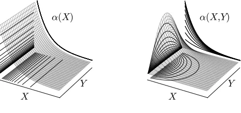
tion at the source together with passive diffusion and a constant auxin bulk degradation away from the source. In [27] the auxin gradient is included in the ROP finite-element numerical simulation after a steady-state is attained. Since we are primarily interested in the biochemical interactions that promote RHs and key ingredients that geometrical features have on the RHs initiation dynamics, rather than providing a detailed model of auxin transport in the cell, we shall hypothesize specific, but qualitatively reasonable in the sense described below, time-independent spatially varying expressions for the auxin distribution in a 2-D azimuthal projection of a 3-D RH cell wall. In this way, we capture crucial ingredients of the spatially-dependent auxin distribution in the cell. Qualitatively, since a RH cell is an epidermal cell, influx and efflux biochemical gates are distributed along the cell membrane, and the auxin flux is known to be primarily directed from the tip of the cell towards the elongation zone (cf. [16,21]), leading to a longitudinally spatially decreasing auxin distribution. Our specific form for the auxin distribution will incorporate such a longitudinal spatial dependence. However, as an extension to the auxin model developed in [4, 6], here we also can take into account non-RH lateral contributions of auxin flux in RH cells by considering an auxin distri-bution with a transverse spatial dependence. This assumption arises as non-RH cells are believed to promote auxin transversal flux into RH cells. However, although auxin is believed to follow pathways either through the cytoplasm or through cell walls of adjacent cells, we are primarily interested in the former pathway that is directed within the cell, and which induces the biochemical switching process (cf. [31]). In this new 2-D analysis of the RD model, we will allow for an auxin distribution that has an ar-bitrary spatial dependence. However, in illustrating our 2-D theory, and motivated by the biological framework discussed above, we will focus on two specific forms for the auxin distribution, as shown in Figure 1: a 1-D form that has the spatially decreas-ing longitudinal dependence of [4, 6], and a modification of this 1-D form that allows for a transverse dependence. We will show that these specific auxin gradients induce an alignment of localized regions of elevated ROP concentration, referred to here as spots. The RD system under consideration exhibits spot-pinning phenomena, in the sense that the position of spots in the stationary patterns is determined by the spatial gradient of auxin. As we shall see below, spots slowly drift until they become aligned with the longitudinal axis of the cell. Their steady-state locations along this cell-midline are at locations determined by the auxin gradient, which effectively “pins” the spots. A similar pinning phenomenon is found for spatially localized structures in other sys-tems: an example is the vortex-pinning phenomenon in the Ginzburg–Landau model of superconductivity in an heterogeneous medium, see [1].

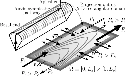
In Figure 2, a sketch of an idealized 3-D RH cell is shown. In this figure,

heav-ily dashed gray lines represent the RH cell membrane. The auxin flux is represented by black arrows, which schematically illustrates a longitudinal decreasing auxin path-way through adjacent cells. As ROP activation is assumed to occur near the cell wall and transversal curvature of the domain is not included in our model, we consider a projection onto a 2-D rectangular domain of this cell, as is also shown inFigure 2.

(3)

X

Y

α

(

X

)

X

Y

[image:3.612.149.385.117.228.2]

α

(

X,Y

)

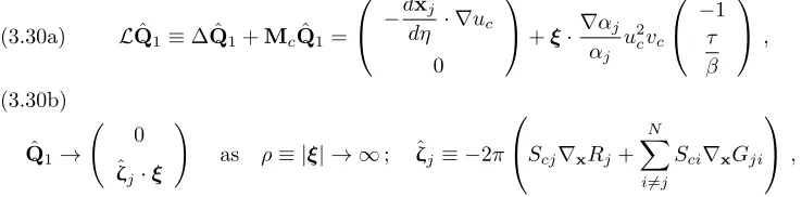
Figure 1. Sketches of the spatially-dependent auxin gradient forms: constant in the transverse direction (left-hand panel), and decreasing on either side of the middle of the cell (right-hand panel).

growth (cf. [22]). In [6] a linear stability analysis showed that multiple-active-ROP 1-D spikes may be linearly stable onO(1) time-scales to 1-D perturbations, with the stability properties depending on an inversely proportional relationship between length and auxin catalytic strength. This dynamic phenomenon is a consequence of an auxin catalytic process sustaining cell wall softening as the RH cell grows. For further discussion of this correlation between growth and biochemical catalysis see [6].

In [4] the linear stability of 1-D stripe patterns of elevated ROP concentration to 2-D spatially transverse perturbations was analyzed. There it was shown that single interior stripes and multi-stripe patterns are unstable under small transverse perturbations. The loss of stability of the stripe pattern was shown to lead to more intricate patterns consisting of spots, or a boundary stripe together with multiple spots (see Figure 9 of [4]). Moreover, it was shown that a single boundary stripe can also lose stability and lead to spot formation in the small diffusivity ratio limit.

Our main new goal in this paper is to analyze these 2-D spot patterns, which results from the breakup of a stripe, and characterize their slow evolution towards a true steady-state of the RD system. In particular, we will examine how specific forms of the auxin gradient lead to a steady-state spot pattern where the spots are aligned with the direction of the auxin gradient.

In the RD model below, U(X, T) and V(X, T) denote active- and inactive-ROP densities, respectively, at timeT >0 and pointX= (X, Y)∈Ω˜ ⊂_R2_{, where ˜}_{Ω is the} rectangular domain ˜Ω = [0, Lx]×[0, Ly]. The on-and-off switching interaction is assumed

to take place on the cell membrane, which is coupled through a standard Fickian-type diffusive process for both densities (cf. [6, 33]). Although RH cells are flanked by non-RH cells (cf. [17]), there is in general no exchange of ROPs between them. Therefore, no-flux boundary conditions are assumed on ∂Ω. On the other hand, we will consider˜ two specific forms for the spatially-dependent dimensionless auxin distributionα: (i) a steady monotone decreasing longitudinal gradient, which is constant in the transverse direction, and (ii) a steady monotone decreasing longitudinal gradient, which decreases on either side of the midlineY =Ly/2; see the left- and right-hand panels inFigure 1,

respectively. These two forms are modelled by

(i) α(X) = exp

−νX

Lx

, (ii) α(X) = exp

−νX

Lx

sin

_πY

Ly

(4)

ˆ n

Pi

]

×

[0

, L

y

]

Apical end

Basal end

Auxin symplastic pathway

[image:4.612.127.392.100.264.2]

Projection onto a 2-D rectangular domain

Figure 2.Sketch of an idealized 3-D RH cell with longitudinal and transversal spatially-dependent auxin flow. The auxin gradient is shown as a consequence of in- and out-pump mechanisms. InfluxPi and effluxPepermeabilities are respectively depicted by the direction of the arrow; the auxin symplastic pathway, indicated by black solid arrows in the 3-D RH cell, is the auxin pathway between cells. Here, the cell membrane is depicted by heavily dashed gray lines. The gradient is coloured as a light gray shade, and auxin gradient level curves are plotted in gray. Cell wall and cell membrane are coloured in dark and light gray respectively. Modified figure reproduced from [6].

As formulated in [4] and [6], the basic dimensionless RD model is

Ut=ε2∆U+α(x)U2V −U+ (τ γ)−1V, x∈Ω,

(1.2a)

τ Vt=D∆V −V + 1−τ γ α(x)U2V −U−βγU, x∈Ω,

(1.2b)

with homogeneous Neumann boundary conditions, and where Ω = [0,1]×[0, dy]. Here

∆ is the 2-D Laplacian, and the domain aspect ratiody ≡Ly/Lx is assumed to satisfy

0 < dy <1, which represents a cell as is shown in Figure 2. The other dimensionless

parameters in(1.2)are defined in terms of the original parameters, as in [4,6], by

ε2≡ D1

L2

x(c+r)

, D≡ D2

L2

xk1

, τ≡ c+r

k1 , β ≡ r k1, (1.3a)

and the primary bifurcation parameterγ in this system is given by

γ≡(c+r)k

2 1 k20b2 . (1.3b)

In the original dimensional model of [6], D1 D2 are the diffusivities for U and V, b is the rate of production of inactive ROP (source parameter), c is the rate constant for deactivation, r is the rate constant describing active ROPs being used up in cell softening and subsequent hair formation (loss parameter), and the activation step is assumed to be proportional to k1V +k20α(x)U2V. The activation and overall auxin level within the cell, initiating an autocatalytic reaction, is represented by k1 > 0 and k20 > 0 respectively. The parameterk20, arising in the bifurcation parameter γ

of (1.3b), will play a key role for pattern formation (see [6,33] for more details on the

model formulation).

(5)

Parameter Set A Parameter Set B

Original Re-scaled Original Re-scaled

D1= 0.075 ε2= 1.02×10−4 D1= 0.1 ε2= 3.6×10−4

D2= 20 D= 0.51 D2= 10 D= 0.4

k1= 0.008 τ = 18.75 k1= 0.01 τ = 11

b= 0.008 β= 6.25 b= 0.01 β= 1

c= 0.1 c= 0.1

r= 0.05 r= 0.01

k20∈

[10−3_,_2.934] γ∈[150,0.051] k20∈[0.01,1.0] γ∈[11,0.11] Lx= 70 Lx= 50

Ly= 29.848 dy= 0.4211 Ly= 20 dy= 0.40

Table 1

Two parameter sets in the original and dimensionless re-scaled variables. The fundamental units of length and time areµm and sec, and concentration rates are measured by an arbitrary datum (con) per time unit;k20 is measured by con2/s, and diffusion coefficients units areµm/s2.

where the active-ROP has an elevated concentration. This analysis is an extension to the analysis performed in [4], where it was shown that a 1-D localized stripe pattern of active-ROP in a 2-D domain will, generically, exhibit breakup into spatially local-ized spots. To analyze the subsequent dynamics and stability of these locallocal-ized spots in the presence of the auxin gradient, we will extend the hybrid asymptotic-numerical methodology developed in [25, 35] for prototypical RD systems with spatially homo-geneous coefficients. This analysis will lead to a novel finite-dimensional dynamical system characterizing slow spot evolution. Although in our numerical simulations we will focus on the two specific forms for the auxin gradient in(1.1), our analysis applies to an arbitrary gradient.

The outline of the paper is as follows. Insection 2we introduce the basic scaling for

(1.2), and we use singular perturbation methods to construct anN-spot quasi

steady-state solution. In section 3 we derive a differential algebraic system (DAE) of ODEs coupled to a nonlinear algebraic system, which describes the slow dynamics of the centers of a collection of localized spots. In particular, we explore the role that the auxin gradient (i) in(1.1)has on the ultimate spatial alignment of the localized spots that result from the breakup of an interior stripe. For the auxin gradient (i) of (1.1), in

section 4 we study the onset of spot self-replication instabilities and otherO(1)

time-scale instabilities of quasi steady-state solutions. Insection 5we examine localized spot patterns for the more biologically realistic model auxin (ii) of (1.1). To illustrate the theory, throughout the paper we perform various numerical simulations and numerical bifurcation analyses using the parameter sets in Table 1, which are qualitatively close to the biological parameters (see [6,33]). Finally, a brief discussion is given insection 6.

2. Asymptotic Regime for Spot Formation. We shall assume a shallow, ob-long cell, which will be modelled as a 2-D flat rectangular domain, as shown inFigure 2. In this domain, the biochemical interactions leading to an RH initiation process are as-sumed to be governed by the RD model(1.2).

(6)

change slowly in time. However, depending on the parameter regime, these localized patterns can also exhibit fastO(1) time-scale instabilities, leading either to spot creation or destruction. For prototypical RD systems such as the Gierer–Meinhardt, Gray–Scott, Schnakenberg, and Brusselator models, the slow dynamics of localized solutions and the possibility of self-replication and competition instabilities, leading either to spot creation or destruction, respectively, have been studied using a hybrid asymptotic-numerical approach in [26,35]. In addition, in the large inhibitor diffusion limit, a leading-order-in-−1/logεanalysis, shows that the linear stability problem for localized spot patterns characterizing competition instabilities can be reduced to the study of classes of nonlocal eigenvalue problems (NLEPs) (cf. [37, 38]). In a 1-D context, rigorous results for the spectral properties of “far-from-equilibrium” periodic 1-D patterns have been obtained recently in [11].

Our previous studies in [6] of 1-D spike patterns and in [4] of 1-D stripe patterns have extended these previous NLEP analyses of prototypical RD systems to the more complicated, and biologically realistic, plant root-hair system (1.2). In the analysis below we extend the 2-D hybrid asymptotic-numerical methodology developed in [26,35] for prototypical RD systems to(1.2). The primary new feature in(1.2), not considered in these previous works, is to analyze the effect of a spatial gradient in the right-hand sides of(1.2), which represents variations in the auxin distribution. This spatial gradient is central to the spatial alignment of the localized structures.

To initiate our hybrid approach for (1.2), we first need to rescale the RD model

(1.2)in Ω in order to determine the parameter regime where localized spots exist. To

do so, we integrate the steady-state version of the RD model(1.2)over the domain to show, as in Proposition 2.2 of [6] for the 1-D problem, that for any steady-state solution U0(x) of (1.2)we must have

Z

Ω

U0(x)dx=

|Ω|

βγ, (2.4)

where |Ω| = dy is the area of Ω. Since the parameters dy, β and γ are O(1), the

constraint(2.4)implies that the average ofU across the whole domain is alsoO(1). In other words, if we seek localized solutions such that U →0 away from localized O(ε) regions near a collection of spots, then from(2.4)we must have thatU =O ε−2near each spot.

2.1. A Multiple-Spot Quasi Steady-State Pattern. In order to derive a finite-dimensional dynamical system for the slow dynamics of active-ROP spots, we must first construct a quasi steady-state pattern describing ROP aggregation inN small distinct spatial regions.

To do so, we seek a quasi steady-state solution whereU is localized within anO(ε) region near each spot locationxj forj= 1, . . . , N. From the conservation law(2.4)we

get thatU =O ε−2and, as a consequence, V =O(ε2) near each spot. In this way, if we replaceU =ε−2_U

j near each spot, and define ξ=ε−1(x−xj), we obtain from

(2.4) that PN

j=1

R

R2Uj dξ ∼ dy/(βγ). This scaling law motivates the introduction of the new variablesuandv defined by

U =ε−2u , V =ε2v . (2.5)

In terms of these new variables,(1.2)with∂nu=∂nv= 0 onx∈∂Ω becomes

ut=ε2∆u+α(x)u2v−u+ε4(τ γ)−1v , x∈Ω,

(2.6a)

τ ε2vt=D0∆v−ε2v+ 1−ε−2

τ γ α(x)u2v−u

+βγu

(7)

whereD=ε−2_D0 _{comes from balancing terms in}_(2.6b)_.

In the inner region near thej-th spot, the leading-order terms in the inner expansion are locally radially symmetric. We expand this inner solution as

(2.7) u=u0j(ρ) +εu1j+· · ·, v=v0j(ρ) +εv1j+· · ·, ρ=|ξ| ≡ε−1|x−xj|.

Substituting (2.7) into the steady-state problem for (2.6), we obtain the following leading-order radially symmetric problem on 0< ρ <∞:

(2.8) ∆ρu0j+α(xj)u02jv0j−u0j= 0, D0∆ρv0j−τ γ α(xj)u20jv0j−u0j−βγu0j = 0,

where ∆ρ≡∂ρρ+ρ−1∂ρ is the Laplacian operator in polar co-ordinates. As a remark,

in our derivation of the spot dynamics insection 3we will need to retain the next term in the Taylor series of the auxin distribution, representing the auxin gradient in the regions where active-ROP is localized. This is given by

(2.9) α(x) =α(xj) +ε∇α(xj)·ξ+· · · , whereξ≡ε−1(x−xj).

These higher-order terms are key to deriving a dynamical system for spot dynamics. We consider(2.8)together with the boundary conditions

(2.10) u0₀_j(0) =v₀0_j(0) = 0 ; u0j →0, v0j∼Sjlogρ+χ(Sj) +o(1), as ρ→ ∞,

whereSjis called thesource parameter. The logarithmic far-field behavior forv0jarises

since, owing to the fact that there is no−v0j term in the second equation of (2.8), we

cannot assume thatv0j is bounded asρ→ ∞. The correction termχj =χ(Sj) in the

far-field behavior is determined from

lim

ρ→∞(v0j−Sjlogρ) =χ(Sj).

(2.11)

By integrating the equation for v0j in (2.8), and using the limiting behavior v0j ∼

Sjlogρas ρ→ ∞, we obtain the identity

Sj=

βγ D0

Z ∞

0

_τ

β α(xj)u 2

0jv0j−u0j+u0j

ρ dρ . (2.12)

In(2.8), we introduce the change of variables

u0j≡

s

D0 βγα(xj)

uc, v0j≡

s

βγ D0α(xj)

vc,

(2.13)

to obtain what we refer to as theshape canonical core problem(SCCP), which consists of

(2.14a) ∆ρuc+u2cvc−uc= 0, ∆ρvc−

τ β u

2

cvc−uc

−uc= 0,

on 0< ρ <∞, together with the following boundary conditions whereScj is a

parame-ter:

(2.14b) u0_c(0) =v_c0(0) = 0, uc→0, vc∼Scjlogρ+χc(Scj) +o(1), as ρ→ ∞.

Upon substituting (2.13) into the identity (2.12), we obtain

Sj≡

s

βγ D0α(xj)

Scj, Scj =

Z ∞

0

τ β u

2

cvc−uc

+uc

(8)

0 1 2 3 4 5 6 4

2 0 2 4 6 8 10

Scj

χc(Scj)

χc(Scj) =3.00170

χc(Scj) =−0.42410

χc(Scj) =−2.33090

(a)

0.0 0.1 0.2 0.3 0.4 0.5 0.6 uuuccc

Scj=2.0

Scj=4.0

Scj=5.0

0 2 4 6 8 10 12

0 2 4 6 8 10

ρ vc

[image:8.612.100.409.101.239.2]

(b)

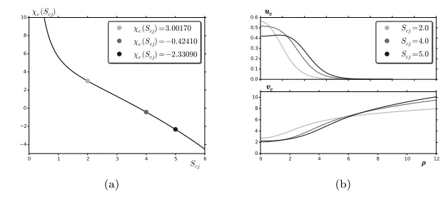
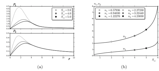
Figure 3. (a) The constantχc(Scj) versus the source parameter Scj, computed numerically from(2.14). (b) Radially symmetric solutionuc(upper panel) andvc(bottom panel), respectively, at the values ofScj shown in the legend. Parameter Set A fromTable 1, whereτ /β= 3.

which, from comparing (2.13) and (2.10), yields

χ(Sj)≡

s

βγ D0α(xj)

χc, where χc=χc(Scj).

(2.15b)

To numerically compute solutions to (2.14) we use the MATLAB code BVP4C

and solve the resulting BVP on the large, but finite, interval [0, ρ0], for a range of values of the parameterScj. The constant χc(Scj) is identified from vc(ρ0)−Sclogρ0=χc,

where vc is the numerically computed solution, and so it depends only on Scj and the

specified ratioτ /β in(2.14). We solve the boundary-value problem on 0< ρ0<12 with a tolerance of 10−4_{. Increasing} _ρ

0 did not change the computational results shown in

Figure 3. The results of our computation are shown inFigure 3(a)where we plotχc(Scj)

versus Scj. InFigure 3(b) we also plot uc and vc at a few values of Scj. We observe

thatuc(ρ) has a volcano-shaped profile whenScj = 5, which suggests, by means of the

identity(2.12), that this parameter value should be near where spot self-replication will occur (seesubsection 4.1).

We remark that the SCCP(2.14)depends only on the ratioτ /β, which characterizes the deactivation and removal rates of active-ROP (see (1.3a)). This implies that the

SCCP (2.14) only describes the aggregation process. On the other hand, notice that

(2.13) and(2.15) reveal the role that the auxin plays on the activation process. Since

α(x) decreases longitudinally for any of the two forms in (1.1), the scaling (2.13) is such that the further from the left boundary active-ROP localizes, the larger will be the solution amplitude. This feature will be confirmed by numerical simulations in

subsection 2.2. In addition, the scaling of the source-parameter in(2.15)indicates that

the auxin controls the inactive-ROP distribution along the cell. That is, while Scj

characterizes how v interacts withuin the region where a spot occurs, the parameter Sjwill be determined by the inhomogeneous distribution of source points, which are also

governed by the auxin gradient. In other words, the gradient controls and catalyzes the switching process, which leads to localized elevations of concentration of active-ROP.

Next, we examine the outer region away from the spots centered at x1, . . . ,xN,

which are locations whereuis localized. To leading-order, the steady-state problem in

(9)

this order in the reaction terms of (2.6b), we obtain in the outer region that

(2.16) −ε2v0+ 1−ε−2

τ γ α(x)u2₀v0−u0

+βγu0

= 1 +O ε2

.

Next, we calculate the effect of the localized spots on the outer equation for v. Upon assuming u ∼ uj and v ∼ vj near the j-th spot, we approximate the singular

terms in the sense of distributions as Dirac masses. Indeed, labelling the reactive terms by Rj ≡τ γ α(x)u2jvj−uj

+βγuj, we use (2.12) and the Mean Value Theorem to

calculate, in the sense of distributions, that

ε−2Rj ε−1(x−xj)→2π

Z ∞

0

Rjj(ρ)ρ dρ

δ(x−xj) = 2πD0Sjδ(x−xj),

(2.17)

asε→0, whereRjj(ρ)≡τ γ α(xj)u20jv0j−u0j

+βγu0j.

Combining(2.16),(2.17)and(2.6b)we obtain that the leading-order outer solution v0, in the region away fromO(ε) neighborhoods of the spots, satisfies

(2.18a) ∆v0+ 1 D0 = 2π

N

X

i=1

Siδ(x−xi), x∈Ω ; ∂nv0= 0, x∈∂Ω.

By using (2.10) to match the outer and inner solutions for v, we must solve (2.18a)

subject to the following singularity behavior asx→xj:

v0∼Sjlog|x−xj|+

Sj

σ +χ(Sj), forj= 1, . . . , N, where σ≡ − 1 logε, (2.18b)

which results from writing (2.10) asρ=ε−1_|_x₋_x

j|.

We now proceed to solve(2.18)forv0and derive a nonlinear algebraic system for the source parametersSc1, . . . , ScN. To do so, we introduce the unique Neumann Green’s

functionG(x;y) satisfying (cf. [26]) ∆G= 1

dy

−δ(x−y),

Z

Ω

G(x;y)dy= 0, x∈Ω, ∂nG= 0, x∈∂Ω.

This Green’s function satisfies the reciprocity relation G(x;y) =G(y;x), and can be globally decomposed asG(x;y) =−1/(2π) log|x−y|+R(x;y), whereR(x;y) is the smooth regular part ofG(x;y). Forx→y, this Green’s function has the local behavior

G(x;y)∼ − 1

2πlog|x−y|+R(y;y) +∇xR(y;y)·(x−y) +O

|x−y|2. An explicit infinite series solution forGandR in the rectangle Ω is available (cf. [26]).

In terms of this Green’s function, the solution to(2.18a)is

(2.19) v0=−2π

N

X

i=1

SiG(x;xi) + ¯v0, where N

X

i=1 Si=

dy

2πD0.

Here ¯v0 is a constant to be found. The condition on Si in (2.19) arises from the

Divergence Theorem applied to (2.18). We then expand v0 as x → xj and enforce

the required singularity behavior(2.18b). This yields that

Sj

σ +χ(Sj) =−2πSjRj−2π

N

X

i=1

SiGji+ ¯v0, for j = 1, . . . N .

(10)

Here Gji ≡ G(xj;xi) and Rj ≡ R(xj;xj). The system (2.20), together with the

constraint in (2.19), defines a nonlinear algebraic system for the N + 1 unknowns S1, . . . , SN and ¯v0. To write this system in matrix form, we define e ≡ (1, . . . ,1)T,

S≡(S1, . . . , SN)T,χ≡(χ(S1), . . . , χ(SN)T, E ≡eeT/N, and the symmetric Green’s

matrixGwith entries

(G)ii=Ri, (G)ij =Gij, where Gij =Gji.

Then,(2.20), together with the constraint in(2.19), can be written as

(2.21) S+ 2πσGS=σ(¯v0e−χ), eTS= dy 2πD0

.

Left multiplying the first equation in (2.21) byeT_{, and using the second equation in}

(2.21), we find an expression for ¯v0

¯ v0=

1 Nσ

_d

y

2πD0+ 2πσe

T_GS₊_σeT_χ

. (2.22)

Substituting ¯v0 back into the first equation of (2.21), we obtain a nonlinear system for S1, . . . , SN given by

S+σ(I−E) (2πGS+χ) = dy 2πN D0e. (2.23)

In terms ofS, ¯v0is given in(2.22). To relateSjandχj with the SCCP(2.14), we define

α≡diag _p 1

α(x1), . . . , 1

p

α(xN)

!

, Sc≡



 

Sc1 .. . ScN





, χc ≡



 

χc(Sc1)

.. . χc(ScN)





.

Then, by using(2.15), we find

S=ωαSc, χ=ωαχc, ω≡

r

βγ D0

. (2.24)

Finally, upon substituting(2.24)into (2.23)we obtain our main result regarding quasi steady-state spot patterns.

Proposition 1. Let 0 < ε 1 and assume D0 = O(1) in (2.6) so that D =

O ε−2

in(1.2). Suppose that the nonlinear algebraic system for the source parameters,

given by

αSc+σ(I−E) (2πGαSc+αχc) =

dy

2πωN D0e, (2.25a)

¯ v0= 1

Nσ

dy

2πD0 + 2πωe

T_GαS

c+σωeTχc

, (2.25b)

has a solution for the given spatial configuration x1, . . . ,xN of spots. Then, there is a

quasi steady-state solution for (1.2)with U =ε−2_u _and_V ₌_ε2_{v. In the outer region} away from the spots, we have u=O(ε4₎ _and_v _∼_{v0, where} _v0 _{is given asymptotically} in terms ofS=ωαSc by (2.19). In contrast, in the j-th inner region nearxj, we have

u∼ s

D0 βγα(xj)

uc, v∼

s

βγ D0α(xj)

vc,

(2.26)

(11)

0 10 20 30 40 50 60 70 0 5 10 15 20 25 Y X t =92.46

0 10 20 30_{40 50 60 70 0 5}10152025 02 4 68 10 12 14 X Y U

0 10 20 30_{40 50 60 70 0 5}10152025 02 4 68 10 12 14 X Y U (a)

0 10 20 30 40 50 60 70

0 5 10 15 20 25 Y X t =240.55

0 10 20 30_{40 50 60 70 0 5}10152025 0 2 46 8 1012 14 X Y U

0 10 20 30_{40 50 60 70 0 5}10152025 0 2 46 8 1012 14 X Y U (b)

0 10 20 30 40 50 60 70

0 5 10 15 20 25 Y X t =25799.11

0 10 20 30_{40 50 60 70 0 5}10152025 02 4 68 10 12 14 X Y U

0 10 20 30_{40 50 60 70 0 5}10152025 02 4 68 10 12 14 X Y U (c)

0 10 20 30 40 50 60 70

0 5 10 15 20 25 Y X t =50000.00

0 10 20 30_{40 50 60 70 0 5}10152025 0 2 46 8 1012 14 X Y U

[image:11.612.124.392.96.369.2]

0 10 20 30_{40 50 60 70 0 5}10152025 0 2 46 8 1012 14 X Y U (d)

Figure 4. Breakup instability of an interior localized homoclinic stripe for U, and the resulting slow spot dynamics. (a) The localized stripe initially breaks into two spots; (b) once formed, the spots migrate from the boundary towards each other in the vertical direction, and then (c) rotate until they get aligned with the longitudinal direction. (d) Finally, they get pinned far from each other along the y-midline by the auxin gradient. Parameter Set A fromTable1 was used withk20= 0.5. For these

values the initial steady-state stripe is centered atX0= 24.5. Figure from [4].

2.2. Spots and Baby Droplets. Proposition 1provides an asymptotic charac-terization of a N-spot quasi steady-state solution. As has been previously studied in the previous paper [4], localized spots can be generated by the breakup of a straight homoclinic stripe. The numerical simulations inFigure 4, for the 1-D auxin gradient in

(1.1), illustrate how small spots are formed from the breakup of an interior homoclinic

stripe and how they evolve slowly in time to a steady-state two-spot pattern aligned with the direction of the auxin gradient. The initial condition for these simulations is obtained by trivially extending a 1-D spike in the transversal direction to obtain a ho-moclinic stripe, which is a steady-state of(1.2), and then perturbing it with a transverse perturbation of small amplitude. As shown in Figure 4(c)–Figure 4(d), the amplitude of the left-most spot decreases as the spot drifts towards the left domain boundary at X = 0, while the amplitude of the right-most spot grows as it drifts towards the right domain boundary atX =Lx. The spot profiles are described byProposition 1for each

fixed re-scaled variables xj. Our realizations of the asymptotic theory shown below in

Figure 7 confirm the numerical results in Figure 4(d) that the spots become aligned

with the direction of the auxin gradient.

In order to explore solutions that bifurcate from a multi-spot steady state, we adapted the _MATLAB code of [2, 34] and performed a numerical continuation for the RD system (1.2) in the bifurcation parameter k20, starting from the solution in

(12)

0.5 1.0 1.5 2.0 40

45 50 55 60

A

B P

LP

BP

k20

||U||2

U

[image:12.612.99.414.94.367.2]

(d)

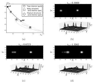
Figure 5.(a) Bifurcation diagram ask20is varied showing a stable branch, labelled A, of (b) two

spots, and unstable branches (light gray-dashed curves). Filled circle atk20o = 0.2319is a fold

bifurca-tion (LP) and the filled star atk∗20= 0.90161is a pitchfork bifurcation (BP). (c) A peanut structure

and one spot steady-state, from label P in (a). (d) A two-spot with baby droplets steady-state solution, from label B in (a). Parameter Set A was used, as given inTable1. Thek20values are shown on top

of upper panels in (b)-(d).

are shown in Figure 5. In the bifurcation diagram depicted inFigure 5(a)the linearly stable branch is plotted as a solid curve and unstable ones by light gray-dashed curves. We found fold bifurcations and a pitchfork bifurcation, represented by a filled circle and a filled star, respectively. To the right of the pitchfork bifurcation, the symmetric solution branch destabilises; the emerging branch of asymmetric states is fully unstable, and features a sequence of fold bifurcations. Overall, these results suggest that a snaking bifurcation structure occurs in 2-D domains, similar to what was found in [4] for the corresponding 1-D system. This intricate branch features a set of fold points (not explicitly labelled in Figure 5(a)), and around each of them a new spot emerges. A pattern consisting of a spot and a peanut structure is found in the solution branch labelled as P. This solution is shown inFigure 5(c).

We found that solutions with peanut structures or baby droplets are unstable steady-states in this region of parameter space, and so they do not persist in time; see a sample of these in Figure 5(d). In addition, as can be seen inFigure 5(b), there are stable multi-spot solutions when k20 is small enough. Overall, this suggests that certain O(1) time-scale instabilities play an important role in transitioning between steady-state patterns (cf. [8, 20]). Further, in section 4, peanut-splitting instabilities are addressed.

(13)

x1, . . . ,xN of localized patches of active-ROP. In this section, we derive a

differential-algebraic system of ODEs (DAE) for the slow time-evolution ofx1, . . . ,xN towards their

equilibrium locations in Ω. This system will consist of a constraint that involves the slow time evolution of the source parametersSc1, . . . , ScN. The derivation of this DAE

system is an extension of the 1-D analysis of [6].

To derive the DAE system, we must extend the analysis in subsection 2.1 by re-taining theO(ε) terms in(2.7)and(2.9). By allowing the spot locations to depend on a distinguished limit for the slow time scale η =ε2t as xj =xj(η), we obtain in the

j-th inner region that the corrections termsu1j and v1j to the SCCP(2.14)satisfy

∆Q1+MQ1=F≡



 −dxj

dη · ∇u0j 0



+ (ξ· ∇αj)u20jv0j

  −1 τ γ D0  , (3.27a)

where the vectorQ1and the matrix Mare defind by

Q1≡

u1j

v1j

, M≡ 



2αju0jv0j−1 αju20j

−τ γ

D0(2αju0jv0j−1)− βγ D0 −

τ γ D0αju

2 0j



 .

(3.27b)

Here αj ≡α(xj) and ∇αj ≡ ∇α(xj). To determine the far-field behavior forQ1, we

expand the outer solutionv0in(2.19)asx→xj and retain theO(ε) terms. This yields

(3.27c) Q1→ 0

ζj·ξ

!

, as ρ≡ |ξ| → ∞,

where, in terms of the source strengthsSj defined from(2.23), we have

(3.27d) ζj ≡ −2π



Sj∇xRj+

N

X

i6=j

Si∇xGji



, j = 1, . . . , N .

Here∇xRj≡ ∇xR(xj;xj) and∇xGj≡ ∇xG(xj;xj) forj= 1, . . . , N.

To impose a solvability condition on (3.27), which will lead to ODEs for the spot locations, we first rewrite(3.27)in terms of the canonical variables(2.13)of the SCCP

(2.14). Using this transformation, the right-hand sideFof (3.27a)becomes

(3.28) F=

s D0 βγαj     −dxj

dη · ∇uc 0



+ξ·

∇αj

αj

u2_cvc

  −1 τ γ D0    .

In addition, the matrixMon the left-hand side of (3.27a)becomes

M=



  

2ucvc−1

D0 βγu 2 c − 1 D0

(τ γ(2ucvc−1) +βγ) −

τ βu 2 c     . (3.29)

Together with(3.28)this suggests that we define new variables ˆu1 and ˆv1 by

u1j≡

s

D0 βγαj

ˆ

u1, v1j≡

(14)

In terms of these new variables, and upon substituting(3.28)and(3.29)into(3.27), we obtain that ˆQ1≡(ˆu1,v1)ˆ T in ξ∈R2 satisfies

LQ1ˆ ≡∆ ˆQ1+McQ1ˆ =



 −dxj

dη · ∇uc 0



+ξ·

∇αj

αj

u2_cvc



 −1

τ β



,

(3.30a)

ˆ

Q1→ 0

ˆ ζj·ξ

!

as ρ≡ |ξ| → ∞; ζˆj ≡ −2π



Scj∇xRj+

N

X

i6=j

Sci∇xGji



,

(3.30b)

and Scj for j = 1, . . . , N satisfies the nonlinear algebraic system(2.25a). In addition,

in(3.30a)Mc is defined by

Mc ≡





2ucvc−1 u2c

−τ

β (2ucvc−1)−1 − τ βu

2

c



,

(3.30c)

whereuc andvc satisfy the SCCP (2.14), which is parametrized byScj.

In(3.30b), the source parameters Scj depend indirectly on the auxin distribution

through the nonlinear algebraic system (2.25), as summarized in Proposition 1. We further observe from the second term on the right-hand side of(3.30a)that its coefficient

∇αj/αj is independent of the magnitude of the spatially inhomogeneous distribution of

auxin, but instead depends on the direction of the gradient.

3.1. Solvability Condition. We now derive a DAE system for the spot dynamics by applying a solvability condition to(3.30). We labelξ= (ξ1, ξ2)T anduc≡(uc, vc)T.

Differentiating the core problem(2.14a)with respect to theξi, we get

L(∂ξiuc) =0, where ∂ξiuc≡

u0_c(ρ) v0_c(ρ)

!

ξi

ρ , for i= 1,2.

[image:14.612.72.441.135.226.2]

This demonstrates that the dimension of the nullspace of L in (3.30), and hence its adjoint L?_{, is at least two-dimensional. Numerically, for our two parameter sets in}

Table 1, we have checked that the nullspace ofL is exactly two-dimensional, provided

thatSj does not coincide with the spot self-replication threshold given insubsection 4.1.

There are two independent nontrivial solutions to the homogeneous adjoint problem

L?_Ψ_≡_∆Ψ₊_MT

cΨ=0given byΨi≡P(ρ)ξi/ρfori= 1,2, wherePsatisfies

(3.31) ∆ρP−

1

ρ2P+M

T

cP=0, 0< ρ <∞; P∼

0

1/ρ

!

as ρ→ ∞.

Here the condition at infinity in(3.31)is used as a normalization condition forP. Next, to derive our solvability condition we use Green’s identity over a large disk Ωρ0 of radius|ξ|=ρ01 to obtain for i= 1,2 that

(3.32)

lim

ρ0→∞ Z

Ωρ0

ΨTiLQ1ˆ −Q1ˆ L ?

Ψi

dξ= lim

ρ0→∞ Z

∂Ωρ0

ΨTi∂ρQ1ˆ −Q1∂ˆ ρΨi ρ=ρ0

dS .

(15)

using(3.30a)to obtain withP≡(P1(ρ), P2(ρ))T _and_x0

j≡(x0j1, x0j2)T that LHS = lim

ρ0→∞ Z

Ωρ₀

−ΨT_i x

0 j· ∇uc

0

!

+ΨT_i

ξ·∇αj

αj

₋₁

τ /β

!

u2_cvc

!

dξ

= lim

ρ0→∞ "

− Z

Ωρ0

P1ξi ρ

2

X

k=1

x0jku0c(ρ)

ξk

ρ dξ+

∇αj

αj

· Z

Ωρ0 ξ

−P1+τ βP2

ξi

ρu 2

cvcdξ

#

,

= lim

ρ0→∞ "

−x0_ji

Z

Ωρ0

P1 ξ2

i

ρ2u

0

c(ρ)dξ+

(∇αj)i

αj

Z

Ωρ0

ξ2

i

ρ

−P1+

τ βP2

u2_cvcdξ

#

,

=−x0jiπ

Z ∞

0

P1u0c(ρ)ρ dρ+

π(∇αj)i

αj

Z ∞

0

−P1+τ βP2

u2cvcρ2dρ ,

wherex0_j=dxj/dη. In deriving the result above, we used the identityR_Ω

ρ0

ξiξkf(ρ)dξ=

δikπ

Rρ0

0 ρ

3_f_(ρ)_{dρ, for any radially symmetric function}_f_{(ρ), where}_δ

ikis the Kronecker

delta.

Next, we calculate the right-hand side (RHS) of(3.32)using the far-field behaviors of ˆQ1 andPas ρ→ ∞. We derive that

RHS = lim

ρ0→∞ Z

∂Ωρ₀

P2yi ρ∂ρ

ˆ ζj·ξ

−ˆζj·ξ∂ρ

P2ξi ρ

dS ,

= lim

ρ0→∞ Z

∂Ωρ0

P2ξ 2

i

ρ2ˆζji−

ˆ ζj·ξ

ξ_i

ρ∂ρP2

dS= lim

ρ0→∞ Z

∂Ωρ0

2ξ_i2

ρ3 ˆζjidS= 2πζˆji.

In the last passage, we used dS =ρ0dθ where θ is the polar angle. Finally, we equate LHS and RHS fori= 1,2, and write the resulting expression in vector form:

(3.33) −x0jπ

Z ∞

0

P1u0cρ dρ+π

∇αj

αj

Z ∞

0

τ

βP2−P1

u2cvcρ2dρ= 2πˆζj.

We summarize our main, formally-derived, asymptotic result for slow spot dynamics as follows:

Proposition 2. Under the same assumptions asProposition 1, and assuming that

theN-spot quasi steady-state solution is stable on anO(1)time-scale, the slow dynamics on the long time-scale η = ε2_t _{of this quasi steady-state spot pattern consists of the} constraints (2.25) coupled to the following ODEs forj= 1, . . . , N:

(3.34a) dxj dη =n1

ˆ ζj+n2

∇αj

αj

, ˆζj≡ −2π



Scj∇xRj+

N

X

i6=j

Sci∇xGji



.

The constants n1 and n2, which depend on Scj and the ratio τ /β are defined in terms

of the solution to the SCCP (2.14) and the homogeneous adjoint solution (3.31) by

n1≡ −_Z ∞ 2

0

P1u0cρ dρ

, n2≡

Z ∞

0

τ

βP2−P1

u2_cvcρ2dρ

Z ∞

0

P1u0cρ dρ

. (3.34b)

In(3.34a), the source parametersScjsatisfy the nonlinear algebraic system(2.25), which

(16)

0.0 0.5 1.0 1.5 2.0 2.5 3.0 3.5 4.0 4.5 PPP111

Scj=2.0

Scj=4.0

Scj=5.0

0 2 4 6 8 10 12

0.0 0.1 0.2 0.3 0.4 0.5

ρ P2

(a)

1 2 3 4 5 6

0 1 2 3 4 5 6 7 8

n2

n1

Scj

n1,n2

n1=0.57936 n1=0.94030 n1=1.22270

n2=2.27230 n2=3.22440 n2=4.23030

[image:16.612.101.408.101.238.2]

(b)

Figure 6. (a) Numerical solution of the adjoint solution satisfying(3.31) forP= (P1, P2)T for

values ofScjas shown in the legend;P1 (top panel) andP2 (bottom panel). (b) Numerical results for

the solvability condition integralsn1 and n2, defined in (3.34b), asScj increases. The filled circles correspond toScj values in (a). We use Parameter Set A fromTable1, for whichτ /β= 3.

Proposition 2describes the slow dynamics of a collection ofNlocalized spots under

an arbitrary, but smooth, spatially-dependent auxin gradient. It is an extension of the 1-D analysis of spike evolution, considered in [6]. The dynamics in(3.34a), shows that the spot locations depend on the gradient of the Green’s function, which depends on the domain Ω, as well as the spatial gradient of the auxin distribution. In particular, the spot dynamics depends only indirectly on the magnitude of the auxin distribution α(xj) through the source parameterScj. The auxin gradient∇αj, however, is essential

to determining the true steady-state spatial configuration of spots. In addition, the spatial interaction between the spots arises from the terms in the finite sum of (3.34a), mediated by the Green’s function. Since the Green’s function and its regular part can be found analytically for a rectangular domain (cf. [26]), we can readily use (3.34) to numerically track the slow time-evolution of a collection of spots for a specified auxin gradient.

Before illustrating results from the DAE dynamics, we must determine n1 andn2 as a function ofScj for a prescribed ratioτ /β. This ratio is associated with the linear

terms in the kinetics of the original dimensional system (1.2), which are related to the deactivation of ROPs and production of other biochemical complexes which promote cell wall softening (cf. [6, 33]). To determinen1 and n2, we first solve the adjoint problem

(3.31) numerically using the MATLAB routine BVP4C. This is done by enforcing

the local behavior that P = O(ρ) as ρ → 0 and by imposing the far-field behavior for P, given in (3.31), at ρ = ρ0 = 12. In Figure 6(a) we plot P1 and P2 for three values of Scj, where τ /β = 3, and Parameter Set A in Table 1 was used. For each

of the three values of Scj, we observe that the far-field behavior P2(ρ) ∼ 1/ρ and P1(ρ)∼(τ /β−1)/ρasρ→ ∞, which is readily derived from(3.31), is indeed satisfied. Upon performing the required quadratures in(3.34b), inFigure 6(b)we plotn1 andn2 versusScj. These numerical results show thatn1>0 andn2>0 forScj >0, which will

ensure existence of stable fixed points of the DAE dynamics. These stable fixed points correspond to realizable steady-state spot configurations for our two specific forms for the auxin gradient.

(17)

0 500 1000 1500 2000 0

10 20 30 40 50 60 70

t

X

1

,X

2

X

1

X

₂

Analytics Numerics

0 500 1000 1500 2000

0 5 10 15 20 25

t

Y

1

,Y

2

Y

₁

Y

2

Analytics Numerics

101 ₁₀2 ₁₀3

10-3 10-2 1010-10

101

Absolute error

_X

1

X2

101 ₁₀2 ₁₀3

10-3 10-2 1010-10

101

Absolute error

Y1

[image:17.612.111.414.127.263.2]

Y2

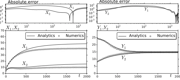
Figure 7.The time-dependent location of two spots for an auxin gradient of the type (i) in(1.1) as obtained from the DAE system (solid curves) inProposition2withk20= 0.3and with parameters

of Parameter Set A ofTable1. The initial locations for the two spots areX1(0) = 7.0,Y1(0) = 8.21

and X2(0) = 3.97, Y2(0) = 24.63. The full numerical results computed from (1.2) are the filled

circles; absolute error in the top panels. Observe that the DAE system predicts that the two spots become aligned along the longitudinal midline of the cell. Thex-coordinate (left-hand panels) and the y-coordinate (right-hand panels) of the two spots.

spot dynamics with corresponding full numerical results computed from (2.6) using a spatial mesh with 500 and 140 gridpoints in the xand y directions, respectively. For the time-stepping a modified Rosenbrock formula of order 2 was used.

The procedure to obtain numerical results from our asymptotic DAE system in

Proposition 2is as follows. This DAE system is solved numerically by using Newton’s

method to solve the nonlinear algebraic system (2.25) together with a Runge–Kutta ODE solver to evolve the dynamics in (3.34a). The solvability integrals n1(Scj) and

n2(Scj) in the dynamics (3.34a) and the function χc in the nonlinear algebraic

sys-tem(2.25)are pre-computed at 200 grid points inScj and a cubic spline interpolation

is fitted to the discretely sampled functions to compute them at arbitrary values ofScj.

For the rectangular domain, explicit expressions for the Green’s functions G and R, together with their gradients, as required in the DAE system, are calculated from the expressions in§4 of [26].

To compare our results for slow spot dynamics we use Parameter Set A ofTable 1

and take k20 = 0.3. For the auxin gradient we took the monotone 1-D gradient in type (i) in(1.1). By a small perturbation of the unstable 1-D stripe solution, our full numerical computations of (2.6)lead to the creation of two localized spots. Numerical values for the centers of the two spots are calculated (see the caption of Figure 7) and these values are used as the initial conditions for our numerical solution of the DAE system in Proposition 2. InFigure 7 we compare our full numerical results for the x and y coordinates for the spot trajectories, as computed from the RD system

(2.6), and those computed from the corresponding DAE system. The key distinguishing

(18)

is computationally expensive to perform more refined numerical simulations over very-long time scales from the full RD system, we are not able to precisely identify why the agreement in the y-coordinate is better than for the x-coordinate. However, overall, the asymptotic theory accurately identifies the time-scale over which the two localized spots become aligned with the auxin gradient along the mid-line of the cell.

4. Fast O(1) Time-Scale Instabilities. We now briefly examine the stability properties of theN-spot quasi-equilibrium solution ofProposition 1toO(1) time-scale instabilities, which are fast relative to the slow dynamics. We first consider spot self-replication instabilities associated with non-radially symmetric perturbations near each spot.

4.1. The Self-Replication Threshold. Since the speed of the slow spot drift is

O(ε2₎_{1, in our stability analysis below we will assume that the spots are “frozen” at} some configurationx1, . . . ,xN. We will consider the possibility of instabilities that are

locally non-radially symmetric near each spot. In the inner region near the j-th spot atxj, whereξ=ε−1(x−xj), we linearize(2.6)around the leading-order core solution

u0j,v0j, satisfying(2.8), by writingu=u0j+eλtφ0j andv=v0j+eλtψ0j. From(2.6),

we obtain to leading order that

∆ξφ0j+α(xj) u02jψ0j+ 2u0jv0jφ0j

−φ0j=λφ0j,

D0∆ξψ0j−τ γ

α(xj) u20jψ0j+ 2u0jv0jφ0j

−φ0j

−βγφ0j = 0,

where ∆ξ is the Laplacian in the local variableξ. Then, upon relatingu0j, v0j to the

SCCP by using (2.13), and defining ψ0j ≡βγψ˜0j/D0, the system above reduces to

(4.35)

∆ξφ0j+ ˜ψ0ju2c+ 2ucvcφ0j−φ0j=λφ0j,

∆ξψ˜0j+

_τ

β −1− 2τ

β ucvc

φ0j−

τ βu

2

cψ˜0j = 0,

whereuc,vc is the solution to the SCCP (2.14).

We then look for an O(1) time-scale instability associated with the local angular integer modem≥1 by introducing the new variables Φ0(ρ) and Ψ0(ρ) defined by

(4.36) φ0j=eimθΦ0(ρ), ψ0˜j =eimθΨ0(ρ), whereρ=|ξ|,ξ=ε−1(x−xj),

andξT =ρ(cosθ,sinθ). Substituting(4.36)into (4.35), we obtain the eigenvalue pro-blem:

(4.37)

LmΦ0+ (2ucvc−1) Φ0+u2cΨ0=λΦ0,

LmΨ0+

_τ

β −1− 2τ

β ucvc

Φ0−τ

βu 2

cΨ0= 0,

0≤ρ <∞.

Here we have definedLmΥ≡∂ρρΥ+ρ−1∂ρΥ−m2ρ−2Υ. We impose the usual regularity

condition for Φ0 and Ψ0 at ρ = 0. The appropriate far-field boundary conditions

for(4.37)is discussed below.

Since the eigenvalue problem (4.37) is difficult to study analytically, we solve it numerically for various integer values of m. We denote λmax to be the eigenvalue of

(4.37)with the largest real part. Sinceucandvcdepend onScjfrom the SCCP(2.14), we

have implicitly thatλmax=λmax(Scj, m). To determine the onset of any instabilities, for

(19)

1 2 3 4 5 6 7 1.0

0.5 0.0 0.5

m=2

m=3

m=4

λmax(Scj,m)

Scj Σ2≈4.16

Σ3≈5.37

Σ4≈6.16

(a)

0.2 0.4 0.6 0.8 1.0 1.2 1.4 1.6 1

2 3 4 5 6

Sc1

Sc2

Σ2≈4.16

k

∗≈20

0

.

85

1

k20 Sc1,Sc2

[image:19.612.97.409.103.238.2]

(b)

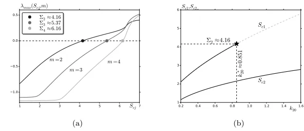
Figure 8. (a) The largest real-valued eigenvalueλmax of (4.37) versusScjfor different angular modesm. The peanut-splitting thresholdsΣmform= 2,3,4are indicated by filled circles. (b) Source parameters for a two-spot steady-state solution of the DAE system (3.34) as k20 is varied. Stable

profiles are the solid curves, and the spot closest to the left boundary atx = 0is unstable to shape deformation on the dashed curve, which begins atk₂₀∗ ≈0.851. This value is the asymptotic prediction of the pitchfork bifurcation point inFigure 5(a)drawn by a filled star. Parameter Set A of Table 1 was used.

In our computations, we only considerm= 2,3,4, . . ., since λmax = 0 for any value of Scj for the translational mode m = 1. Any such instability for m = 1 is reflected in

instability in the DAE system(3.34a).

Form≥2 we impose the far-field behavior that Φ0 decays exponentially asρ→ ∞

while Ψ0 ∼ O(ρ−m₎_→_{0 as}_ρ_{→ ∞}_{. With this limiting behavior,} _(4.37)_{is discretized}

with centered differences on a large but finite domain. We then determineλmax(Scj, m)

by computing the eigenvalues of the discretized eigenvalue problem, in matrix form. For m ≥2 our computations show thatλmax(Scj, m) is real and that λmax(Scj, m)>0 if

and only if Scj > Σm. In our computations we took 400 meshpoints on the interval

0≤ρ <15. For the ratio τ /β = 3, corresponding to Parameter Set A of Table 1, the results for the threshold values Σmform= 2,3,4 given inFigure 8(a)are insensitive to

increasing either the domain length or the number of grid points. Our main conclusion is that as Scj is increased, the solution profile of thej-th spot first becomes unstable

to a non-radially symmetric peanut-splitting mode, corresponding to m = 2, as Scj

increases above the threshold Σ2 ≈ 4.16 when τ /β = 3. As a remark, if we take τ /β = 11, corresponding to Parameter Set B of Table 1, we compute instead that Σ2≈3.96.

To illustrate this peanut-splitting threshold, we consider a pattern with a single localized spot. Using(2.19) we findS1=dy/(2πD0). Then,(2.15)yields the following

expression for the source parameter for the SCCP(2.14)

(4.38) Sc1=

dy

2π

s

α(x1) D0βγ .

(20)

[image:20.612.103.408.98.229.2]

(a) (b)

Figure 9. Two snapshots of a time-dependent numerical simulation where a peanut structure merges into a spot. (a) Peanut structure and a spot. (b) Two spots. Parameter Set A as given in Table1andk20= 0.6723for an auxin gradient of the type (i) in (1.1)

the type (i) in (1.1), this linear peanut-splitting instability triggers a nonlinear spot replication event.

In addition, in Figure 8(b) we plot the source parameters corresponding to the two-spot steady-state aligned along the midline Y = Ly/2 as the parameter k20 is

varied. These asymptotic results, which asymptotically characterize states in branch A

of Figure 5(a), are computed from the steady-state of the DAE system (3.34). Notice

that the spot closest to the left-hand boundary loses stability atk20∗ ≈0.851, when Sc1 meets the peanut-splitting threshold Σ2. On the other hand, Sc2 values corresponding to the spot closest to the right-hand boundary are always below Σ2 for the parameter range considered. Hence, no shape change for this spot is observed. This result rather accurately predicts the pitchfork bifurcation inFigure 5(a)portrayed by a filled star at k∗₂₀≈0.902.

4.2. Numerical Illustrations ofO(1)Time-Scale Instabilities. InFigure 5(c)

we showed a steady-state solution consisting of a spot and a peanut structure, which is obtained from numerical continuation in the parameter k20. This solution belongs to the unstable branch labelled by P in Figure 5(a), which is confined between two fold bifurcations (not explicitly shown). We take a solution from this branch as an initial condition in Figure 9(a) for a time-dependent numerical simulation of the full RD model(1.2)-(2.6)using a centered finite-difference scheme. Our numerical results

in Figure 9(b)show that this initial state evolves dynamically into a stable two-spot

solution. This is a result of the overlapping of the stable branch A with an unstable one in the bifurcation diagram.

Other initial conditions and parameter ranges also exhibitO(1) time-scale instabil-ities. To illustrate these instabilities, and see whether a self-replication spot process is triggered by a linear peanut-splitting instability, we perform a direct numerical simu-lation of the full RD model (1.2) taking as initial condition the unstable steady-state solution labelled by B inFigure 5(a). This steady-state, shown inFigure 10(a), consists of two spots, with one having four small droplets associated with it. This particular steady-state is chosen since both competition and self-replication instabilities can be seen in the time evolution of this initial condition in the panels ofFigure 10. Firstly, we observe inFigure 10(b) that the small droplets for the left-most spot in Figure 10(a)

(21)

(a) (b)

(c) (d)

[image:21.612.101.411.98.503.2]

(e) (f)

Figure 10.Numerical simulations of the full RD system illustratingO(1)time-scale instabilities.

Competition instability: (a) baby droplets and (b) a spot gets annihilated. Spot self-replication: (c) one spot, (d) early stage of a self-replication process, (e) a clearly visible peanut structure, and (f ) two distinct spots moving away from each other. Parameter Set A as given inTable 1andk20= 1.6133.

(22)

Competition and self-replication instabilities, such as illustrated above, are two types of fastO(1) time-scale instabilities that commonly occur for localized spot patterns in singularly perturbed RD systems. Although it is beyond the scope of this paper to give a detailed analysis of a competition instability for our plant RD model(1.2), based on analogies with other RD models (cf. [9, 25,26,35]), this instability typically occurs when the source parameter of a particular spot is below some threshold or, equivalently, when there are too many spots that can be supported in the domain for the given substrate diffusivity. In essence, a competition instability is an overcrowding instability. Alternatively, as we have unravelled insubsection 4.1, the self-replication instability is an undercrowding instability and is triggered when the source parameter of a particular spot exceeds a threshold, or equivalently when there are too few spots in the domain. For the standard Schnakenberg model with spatially homogeneous coefficients, in [26] it was shown through a center-manifold type calculation that the direction of splitting of a spot is always perpendicular to the direction of its motion. However, with an auxin gradient the direction of spot-splitting is no longer always perpendicular to the direction of motion of the spot. In our plant RD model, the auxin gradient not only enhances robustness of solutions, which results in the overlapping of solution branches and is suggestive that a strong slanted homoclinic snaking mechanism can occur (see the next section), but it also controls the location of steady-state spots (see subsection 2.2and

section 3).

5. More Robust 2D Patches and Auxin Transport. We now consider a more biologically plausible model for the auxin transport, which initiates the localization of ROP. This model allows for both a longitudinal and transverse spatial dependence of auxin. The original ROP model, derived in [6,33] and analyzed in [4,6] and the sections above, depends crucially on the spatial gradient of auxin. The key assumption we have made above was to assume a decreasing auxin distribution along theX-direction. Indeed, such an auxin gradient controls the x-coordinate spot location in such a way that the larger the overall auxin parameter k20, the more spots are likely to occur. However, as was discussed insection 4, there are instabilities that occur when an extra spatial dimension is present. In other words, when an RH cell is modelled as a two-dimensional flat and oblong cell, certain pattern formation attributes become relevant that are not present in a 1-D setting. In particular, 1-D stripes generically break up into localized spots, which are then subject to possible secondary instabilities. We now explore the effect that a 2-D spatial distribution of auxin has on such localized ROP spots.

5.1. A 2-D Auxin Gradient. Next, we perform a numerical bifurcation analysis of the RD system(1.2)for an auxin distribution of the form given in (ii) of(1.1). Such a distribution represents a decreasing concentration of auxin in the X-direction, as is biologically expected, but with a greater longitudinal concentration of auxin along the midlineY =Ly/2 of the flat rectangular cell than at the edgesY = 0, Ly.

To perform a numerical bifurcation study we discretize(1.2) using centered finite differences and we adapt the 2-D continuation code written in_MATLABgiven in [34]. We compute branches of steady-state solutions of this system using pseudo arclength continuation, and the stability of these solutions is computed a posteriori using

MAT-LABeigenvalue routines. The resulting bifurcation diagram is shown inFigure 11(a).

(23)

0.00 0.02 0.04 0.06 0.08 0.10 150 200 250 300 350 400 1 2 ₃

||U||2

Boundary patch One interior patch Boundary and one interior patch

0.10 0.15 0.20 0.25 0.30 0.35 0.40 135 140 145 150 155 160 165 170 4 5

||U||2

k20

U

(f)

Figure 11.Bifurcation diagram of the RD system(1.2)in terms of the original parameters while

varyingk20. Hereα=α(X)as given in (ii) of(1.1)in a 2-D-rectangular domain. (a) Stable branches

are the solid lines, and filled circles represent fold points; top and bottom panels show overlapping of branches of each steady solution: (b) boundary spot, (c) one interior spot, (d) boundary and one interior spot, (e) two interior spots, and (f ) boundary and two interior spots. Parameter Set B, as given inTable 1, was used. Thek20 values are given on top of the upper panels for each steady-state

in (b)-(f ).

distinguishing feature: solutions belong to a single branch of steady states, undergoing a sequence of fold bifurcations and, in some cases, a change in stability. In large inter-vals ofk20we observe multistability which, in turn, indicates that hysteretic transitions between solutions with varying number of spots can occur.

To explore fine details of this bifurcation behavior, the bifurcation diagram in

Fig-ure 11(a) has been split into two parts, with the top and bottom panels for lower and

(24)

of Figure 11(a). Ask20 is increased, stability is lost at a fold-point bifurcation which gives rise to branch 2 of Figure 11(a), which gathers a family of single interior spot steady-states, as shown in Figure 11(c). As k20 increases further, this interior spot solution persists until stability is lost at a fold-point bifurcation. Branch 3 in

Fig-ure 11(a)consists of stable steady-states of one interior spot and one boundary spot, as

shown in Figure 11(d). Furthermore, Figure 11(e) shows that steady-states consisting of two interior spots occur at even larger values of k20. This corresponds to branch 4

of Figure 11(a). Finally, at much larger values ofk20, Figure 11(f)shows that an

ad-ditional spot is formed at the domain boundary. This qualitative behavior associated with increasing k20 continues, and leads to a creation-annihilation cascade similar to that observed for 1-D pulses and stripes in [6] and [4], respectively. In other words, over-lapping stable branches yield steady-states consisting of interior and/or boundary spots that appear or disappear ask20 is either slowly increased or decreased, respectively.

5.2. Instabilities with a 2-D Spatially-Dependent Auxin Gradient. Sim-ilar to the 1-D studies in [4, 6], the auxin gradient controls the location and number of 2-D localized regions of active ROP. As the level of auxin increases in the cell, an increasing number of active ROPs are formed, and their spatial locations are controlled by the spatial gradient of the auxin distribution. Moreover, in analogy with the theory of homoclinic snaking, overlapping of stable solution branches occurs, and this leads to a wide range of different observable steady-states in the RD system. These signature features of the bifurcation structure suggest that homoclinic snaking can occur for(1.2), similar to that observed in [5] for a RD system with spatially homogeneous coefficients. In passing, we note that the snaking observed in our system is slanted. Slanted snaking has been reported in systems with conserved quantities (see for instance [10, 36]). The system under consideration does not have a conserved quantity, and the slanting is caused by the auxin gradient. In other words, the gradient gives rise to a strongly slanted homoclinic snaking behavior.

Transitions from unstable to stable branches are determined through fold bifurca-tions, and are controlled byO(1) time-scale instabilities. To illustrate this behavior, we perform a direct numerical simulation of the full RD model(1.2)taking as initial condi-tion an unstable steady-state solucondi-tion consisting of two rather closely spaced spots, as shown inFigure 12(a). The time-evolution of this initial condition is shown in the differ-ent panels ofFigure 12. We first observe from Figure 12(b)that these two spots begin to merge at the left domain boundary. As this merging process continues, a new-born stripe emerges near the right-hand boundary, as shown in Figure 12(c). This interior stripe is weakest at the top and bottom boundaries, due to the relatively low levels of auxin in these regions. InFigure 12(d), the interior stripe is observed to give rise to a transversally aligned peanut structure, which remains centered at theY-midline for the same reasons as above at the top and bottom boundaries, whilst another peanut struc-ture in the longitudinal direction occurs near the left-hand boundary. The right-most peanut structure slowly collapses to a solitary spot, while the left-most form undergoes a breakup instability, yielding two distinct spots, as shown in Figure 12(e). Finally,

Figure 12(f)shows a steady-state solution with three localized spots that are spatially

U

[image:25.612.100.411.96.499.2]

(f)

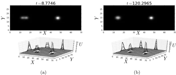
Figure 12. Numerical simulations of the full RD system with the 2-D spatial auxin distribution given by type (ii) of (1.1). The initial condition, shown in (a), is a boundary and interior spot unstable steady-state. The subsequent time-evolution of this steady-state is: (b) spots merging; (c) a new homoclinic stripe is born; (d) a peanut structure emerges; (e) an interior spot arises from a collapsed peanut structure, and (f ) finally, a two interior and one boundary spot stable steady-state. Parameter Set B, as given inTable 1withk20= 0.0209, was used.

to a peanut structure centered near the Y-midline, which then does not undergo a self-replication process but instead leads to the merging, or aggregation, of the peanut structure into a solitary spot. The transverse component of the 2-D auxin distribution is essential to this behavior.

We remark that the asymptotic analysis insection 2andsection 3for the existence and slow dynamics of 2-D quasi steady-state localized spot solutions can also readily be implemented for the 2-D auxin gradient type (ii) of (1.1). The self-replication threshold

insubsection 4.1also applies to a 2-D spatial gradient for auxin. However, for an auxin